White Rose Research Online URL for this paper: http://eprints.whiterose.ac.uk/106787/
Version: Accepted Version
Article:
Korsos, M.B., Ludmany, A., Erdelyi, R. et al. (1 more author) (2015) On flare predictability based on sunspot group evolution. Astrophysical Journal Letters, 802 (2). L21. ISSN 2041-8205
https://doi.org/10.1088/2041-8205/802/2/L21
[email protected] https://eprints.whiterose.ac.uk/
Reuse
Unless indicated otherwise, fulltext items are protected by copyright with all rights reserved. The copyright exception in section 29 of the Copyright, Designs and Patents Act 1988 allows the making of a single copy solely for the purpose of non-commercial research or private study within the limits of fair dealing. The publisher or other rights-holder may allow further reproduction and re-use of this version - refer to the White Rose Research Online record for this item. Where records identify the publisher as the copyright holder, users can verify any specific terms of use on the publisher’s website.
Takedown
If you consider content in White Rose Research Online to be in breach of UK law, please notify us by
arXiv:1503.04634v1 [astro-ph.SR] 16 Mar 2015
M. B. Kors´os1,2
, A. Ludm´any1
, R. Erd´elyi1,2
and T. Baranyi1
[korsos.marianna; baranyi.tunde; ludmany.andras]@csfk.mta.hu
Received ; accepted
1
Debrecen Heliophysical Observatory (DHO), Research Centre for Astronomy and Earth
Sciences, Hungarian Academy of Science, 4010 Debrecen, P.O. Box 30, Hungary
2
Solar Physics & Space Plasma Research Center (SP2RC), University of Sheffield,
ABSTRACT
The forecast method introduced by Kors´os et al. (2014) is generalised from
the horizontal magnetic gradient (GM), defined between two opposite polarity
spots, to all spots within an appropriately defined region close to the magnetic
neutral line of an active region. This novel approach is not limited to searching
for the largest GM of two single spots as in previous methods. Instead, the
pre-flare conditions of the evolution of spot groups is captured by the introduction of
theweightedhorizontal magnetic gradient, orW GM. This new proxy enables the
potential of forecasting flares stronger than M5. The improved capability includes
(i) the prediction of flare onset time and (ii) an assessment whether a flare is
followed by another event within about 18 hours. The prediction of onset time is
found to be more accurate here. A linear relationship is established between the
duration of converging motion and the time elapsed from the moment of closest
position to that of the flare onset of opposite polarity spot groups. The other
promising relationship is between the maximum of theW GM prior to flaring and
the value ofW GM at the moment of the initial flare onset in the case of multiple
flaring. We found that when the W GM decreases by about 54%, then there is
no second flare. If, however, when theW GM decreases less than 42%, then there
will be likely a follow-up flare stronger than M5. This new capability may be
useful for an automated flare prediction tool.
1. Introduction
The endeavour to establish reliable flare forecast methods has resulted in numerous
attempts to identify promising physical quantities, proxies, features and behavioural
patterns to predict an imminent flare (see e.g. Sawyer 1986; Hochedez et al. 2005;
Benz 2008). The ultimate task is to construct a diagnostic tool that determines the
unique conditions leading to flaring events, triggered by magnetic reconnection (see e.g.
Yamada et al. 2010). The empirical study presented here focuses on features at the solar
surface, namely investigating the pre-flare dynamics of sunspot groups.
Most of the attempts that developed flare forecast tools employ suitably defined
(and derived) quantities from magnetograms. The majority of previous efforts studied
the behaviour of the horizontal gradient of the line-of-sight component of the magnetic
field, usually a well-observed property of an active region (AR). By investigating the Solar
and Heliospheric Observatory’s Michelson Doppler Imager (SOHO/MDI) magnetograms,
Schrijver (2007) found that energetic flares are connected to the separation line of opposite
polarity regions with high magnetic gradient. Further works followed suit, including
e.g. Mason & Hoeksema (2010) who studied the gradient-weighted inversion line length
which exhibits a significant increase prior to flares. The maximum horizontal gradient
and the length of the neutral line were considered by Cui et al. (2006), Jing et al.
(2006), Huang et al. (2010) and Yu et al. (2010). The fractal structure was addressed by
Criscuoli et al. (2009), however, Georgoulis (2012) was sceptical about this approach. In
the literature, there are a number of other indicators proposed to measure non-potentiality.
Leka & Barnes (2007) suggested 8 categories of different distributions with an impressive
list of 29 types of variables defined on them. All these methods above (and others)
have advantages and caveats, however, none are yet accepted as a universal and reliable
Surprisingly, sunspots themselves are rarely considered as possible holders of
information for flare forecast. Arguably, the simplest way to apply sunspot data is to
approach non-potentiality by using their McIntosh classification (Bloomfield et al. 2012).
However, the McIntosh classes are only based on morphology, and they do not contain
perhaps the most important information relevant to the present context, i.e. the distribution
of opposite magnetic polarities. Our preceding study (Kors´oset al. 2014, hereafter Paper
I) is the first attempt to track the details of the evolution of sunspots (umbrae) in order to
identify signatures of flare imminence. Paper I implemented a proxy horizontal magnetic
gradient, GM, defined between two single spots of opposite polarities close to the magnetic
neutral line. The pre-flare behaviour of this proxy quantity exhibited characteristic and
unique patterns: steep rise, high maximum and a gradual decrease prior to flaring. These
properties may yield a tool for the assessment of flare probability and intensity within a
2-10 hour window.
The method developed here allows us to elaborate on some of the most important
properties of an imminent flare; its intensity and the onset time. The prediction of
intensity is found to be more reliable, as a linear relationship has been found between the
pre-flare maximum of GM and the peak intensity emitted in the 1-8 ˚A range, according to
Geostationary Operational Environmental Satellite (GOES) x-ray measurements1
. This
result may be considered to be an indicator of the existing relationship between the proxies
of free and released energies. Next, the onset time prediction is found to be somewhat less
precise, as the most probable time of flare onset is between 2 and 10 hours after the GM
maximum. The aim of the present work is to find more reliable forecasting methods for the
onset time as well as the likelihood of consecutive flaring.
1
2. Method of Examination
The empirical basis of this study, similar to Paper I, is the SDD2
(SOHO/MDI-Debrecen
Data) sunspot catalogue, the most detailed of its kind covering the years of MDI operations
(1996-2010). In addition, the intensity peaks of the examined flares the GOES solar flare
database3
is employed. The SDD is efficient for tracking the internal dynamics of spot
groups. It contains data on position, area and magnetic field for all spots with a cadence of
1.5 hrs (Gy˝ori et al. 2011).
Let us now consider the involvement of all magnetic spots in an appropriately selected
area at the region of a Polarity Inversion Line (PIL). When a new spot (min. 3 MSH)
emerges close (within 40 ±5 Mm, which is always enough to capture the emergence) to
existing spots of opposite polarity, we determine the maximum GM between the emerging
and existing spots. Once a pair of spots of opposite polarities with a maximum GM is
found, we compute the area-weighted centre between them. Next, there is a defined circular
area, around this weighted location where GM is highest, whose diameter is 3◦±0.5◦ in
Carrington heliographic coordinates. The center of the circle is fixed and spot groups within
this area are now monitored.
We assume that the underlying process driving a flare is a collective one between
nearby spots. Therefore, a new proxy parameter, a generalisation of the GM, called the
weighted horizontal magnetic gradient (W GM) is defined to account for this collective
behaviour:
W GM =
P
iBp,i·Ap,i−
P
Here, B (determined by f(A) in Paper I) and A denote the mean magnetic field and
area of umbra. The indices p and n denote positive and negative polarities, i and j are
their running indices in the selected spot cluster and dpn is the distance between the
area-weighted centers of two subgroups of opposite polarities in this cluster.
We have analysed 45 single and 16 multiple flare cases which are stronger than M5
between 1996 and 2010. This limitation is based on the findings of Paper I, i.e. the present
method seems to be suitable for energetic flares above M5. Besides some similarities
between the behaviour of GM and W GM, the current approach results in significant,
previously unseen pre-flare behavioural patterns. Let us demonstrate the key features with
two randomly selected, but typical, examples.
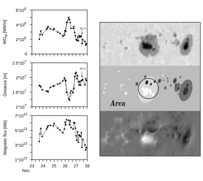
Figure 1 shows a typical active region, AR 8771, with a single flare. The right-hand
panels of Fig. 1 are: the white light image (top), magnetogram (bottom) and a cartoon
reconstructing the AR from the SDD catalogue (middle). The W GM (top left) shows a
steep rise and high maximum (called W Gmax
M ) followed by its decrease until the flare.
However, and most importantly, we found characteristic and appealing differences from
the result of the single spot-pair method, as demonstrated by e.g. the distance diagnostics
panel (middle left) of the spot groups of opposite fluxes. This plot contains a conspicuous
dip, indicating a duration of converging-diverging motion of the area-weighted centres that
seem to be indicative of the next flare for all cases we investigated. The total unsigned
magnetic flux (bottom left) in this part of the AR shows some increase before the flare but
it has no special, identifiable characteristic feature. Additionally, we tested a large sample
of non-flaring spot groups with opposite polarities to determine whether this behaviour
is found in these cases as well. We found no such behaviour. Therefore, the evolution of
the distance between the area-weighted centers of spot groups of opposite polarities shows
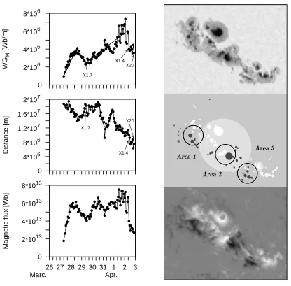
Figure 2 is another typical example, i.e. AR 9393 also examined in Paper I, but now
with multiple flare activities linked only to Area 2 because the highest variability of W GM
is in Area 2, while Area 1 and 3 do not show such a property (see in Paper I). A series of
flares is considered multiple, if after the occurring flare there is another flare, within an
18-hr window, belonging to the same preceding rising phase of W GM and at the same time
belonging to the same decreasing phase after W Gmax
M (see e.g. the X1.4 flare followed by
the X20 flare in the upper left panel of Fig. 2). The behaviour of W GM is analogous to
that of the single spot-pair (compare to GM of Fig. 2 in Paper I), showing a steep rise, high
maximum and a slower decrease prior to the X1.7 single flare (29 March), and, in spite of
the limited temporal resolution, arguably a similar pattern is found leading to the follow-up
ndependent multiple flares (i.e., X1.4 and X20, 2 April). Next, the distance diagnostics
(middle left) panel of the spot groups of opposite fluxes do show similar conspicuous
dips as in Fig. 1. Note, these multiple flares are likely unrelated to the single flare as
they do not fall within the 18-hour window we propose as a requirement for flares to be
connected. Again, this pre-flare behaviour pattern was not identifiable in the distance
diagram of the single spot-pair method in Paper I (see its Fig. 2, left column, middle
panel). Finally, we could not conclude any special and immediate pre-flare behaviour on a
daily time-scale by investigating the variation of unsigned flux within Area 2 (bottom left)
because it was decreasing before the X1.7 flare while it was increasing before the X1.4 flare.
A statistical study also shows that the temporal variation of the unsigned flux does not
exhibit characteristic pre-flare signatures. This, however, does not contradict the findings
of Schrijver (2007) about a statistical relationship between the likelihood of X- or M-flares
and the unsigned flux at SPIL (Strong-gradient Polarity Inversion Line) because selected
actual states of ARs were investigated and not the time profile of the examined quantities.
By the above examples of case studies, we are now encouraged to conduct a statistical
of over M5 available in the SDD catalogue.
3. Diagnostic potentials with spot dynamics
We test the proposed diagnostics on a statistical sample by applying the following
requirements: Firstly, the examined pre-flare variation is within ±70◦ from the central
meridian to avoid geometrical foreshortening close to the limb. Next, the flare onset is no
further eastward from the central meridian than −40◦ to have sufficient time to follow the
development of W GM.
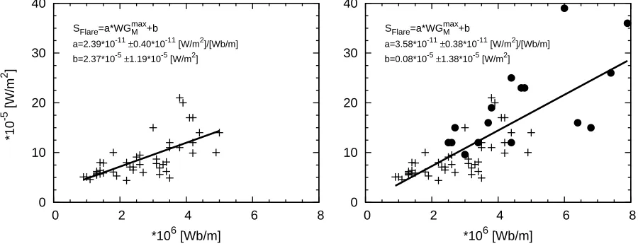
In Paper I, a linear relationship was found between the maximum value of GM
preceding a flare and the peak intensity of flares. This behaviour is confirmed for W GM
by Fig. 3. 45 single flares (crosses, left panel) and 45 single with additional 16 largest of
multiple flares (circles, right panel) show a linear relationship between W Gmax
M and the
corresponding GOES flare intensity. Here, we restrict the empirical analysis for flares
between M5 and X4 classes only.
Next, the new method revealed further important connections, which is conspicuous,
in Figs. 1 and 2. This connection is between the durations of converging-diverging motion
of the centers of opposite polarities. This intriguing pattern was found in all 61 cases
investigated here. The question rises, whether there is a relationship between the duration
of the converging motion (the duration from the moment of the first point when the distance
began decreasing to the moment of the minimum point of the parabolic curve) and the
time elapsed from the moment of minimum distance until the flare onset (duration of the
diverging motion and the follow-up time until the flare onset). To determine these two time
intervals for each flare, parabolic curves were fitted to their distance data. For a sample see
panel of Fig. 1, showing the converging-diverging behaviour of this relative motion.
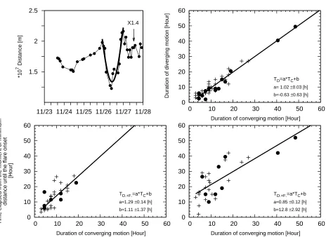
Figure 4 gives further insight into the relation between these intervals by plotting the
time from the moment of minimum distance to the flare onset as a function of the duration
of converging motion. First, the upper right diagram depicts the duration of diverging
motion as function of the duration of converging motion for the 45 single (crosses) and 16
multiple (circles) flare cases. Note that the duration of diverging motion is shorter than
the time period from the moment of minimum distance to that of the flare onset (see
bottom panels of Fig. 4). However, the converging-motion phase and the diverging-motion
phase have the same duration. Yamada et al.(2010) found similar properties in laboratory
reconnection experiments, and called it the ”push and pull-mode”. The present observations
are a confirmation of the laboratory experiment.
The lower diagrams plot the time from the moment of closest position to the flare
onset as function of the duration of the converging motion phase. In the cases of multiple
flares, we investigated the time from the moment of closest position to the first flare onset
as function of the duration of the converging motion phase. The left/right panel contains
those cases when the spot groups are younger/older than three days at the time of flare
onset. The regression lines of the two cases are, surprisingly, different. By estimating the
time the magnetic fields younger than three days should be distinguished from the older
ones, the relevant formulae are given in the lower panels of Figure 4. One may be able to
estimate a rough onset time of the flare. Note the considerable dispersion. If the study area
is younger than three days then about a mere hour is needed to be added to the duration
of the corresponding scaled duration of converging motion, where the scale-factor is 1.3 for
younger ones, to obtain the flare onset time. However, if the area is older than three days
then the scale-factor is 0.85, and one needs to add 12 ±3 hours to the scaled duration of
Next, a relationship is found between the values of W GM at its maximum prior to
flaring (W Gmax
M ) and at the time of flare onset (W GF lareM ), as visualised in Figure 5. We
investigate separately the 45 cases when only a single flare took place after the maximum of
W GM, and the 16 when more flares erupted after the maximum within an 18-hour window
after the occurring flare on the decreasing phase of the W GM. The left panel depicts the
cases of single energetic flares (crosses). The right panel depicts the first flares (circles) of
those ARs where multiple flares are produced. The plots are interpreted as follows: a single
flare erupts when the W Gmax
M was less than 5·10
6
Wb/m and the W GM decreases by more
than half of the W Gmax
M , in the pre-flare phase (for example the X1.4 flare in the NOAA
8771 on Fig. 1 and the X1.7 flare in the AR NOAA 9393 on Fig. 2). This is likely due to
the fact that the magnetic energy in the region decreases so significantly during this first
flare that there is simply not enough energy left to release another flare. In that case, if the
decrease is smaller than half (about 42%) by the onset of the first flare, some further flaring
may be expected, meaning that the disturbance of this first flare could be forcing opposite
polarity fields together in the solar atmosphere leading, for example to the ‘homologous’
flaring that is often observed. On the other hand, the W Gmax
M larger than 5·10
6
Wb/m
seems to be enough in itself to predict a multiple flaring event. We cannot comment yet on
further flares (i.e. third, etc.) in the case of multiple flares as the temporal resolution of the
SDD catalogue is too coarse. For an example, see the case of AR NOAA 9393 where an X
1.4 flare was followed by an X 20 one within 12 hours (Fig. 2).
4. Discussion
In this paper, we present advancements in the classification of pre-flare conditions with
an application to flare prediction. 61 cases were investigated in the vicinity of PILs of ARs.
needs further investigations both observationally (with higher resolution) and theoretically
(e.g. numerical simulations).
First, we found that the pre-flare behaviour of the weighted horizontal magnetic
gradient (W GM) exhibits similar patterns to those found with the single spot-pair method:
steep rise, high maximum and gradual decrease until the flare onset (Figs. 1-2). Next,
Figure 3 corroborates the relationship, reported in Paper I, between the maximum of
GM and the intensity of single flares. Here, this relationship is modelled as linear one,
however, the dispersion is considerable and theoretical (e.g. numerical) modelling may
be necessary to confirm or refute this relation. There may be a yet unknown physical
parameter, therefore not accounted for, that would reduce the dispersion. This is the reason
of restriction on the currently considered GOES classes. However, the relationship found
can be still regarded to be a link between the proxy measures of the free energy and the
released energy. A shortfall of the single spot-pair method was that one could not deduce
the flare intensity in the case of multiple flares. This is now rectified by the introduction
of the weighted horizontal magnetic gradient. The spot-group method is now capable of
providing a rough estimate of the expected largest flare intensity from W Gmax
M (Fig. 3).
In addition, this method also gives a better estimate of the expected time of flare onset
(Fig. 4), and, may be able to predict whether an energetic flare after W Gmax
M is the only
flare or further flare events can be expected (Fig. 5).
Let us assume that W GM is a proxy of the available non-potential (i.e. free) energy to
be released in a spot group. In this case, we may conclude from Fig. 5: (i) if the maximum
of the released energy may be over half of the maximum of the accumulated (free) energy,
no further energetic flare(s) can be expected; (ii) If the maximum of the released flare
energy is less than about ∼42%, further flares are more probable. In short, Fig. 5 allows
consecutive flares and their intensities.
Last but not least we provide some notes on the estimate of the onset time of an
imminent flare. Here, its determination is refined. Paper I only presented a statistics that
60% of observed energetic flares are between 2-10 hrs after the maximum of GM. Figure 4,
however, allows a much stronger statement on the expected time of onset due to W GM.
The figure uncovers the relationship between the duration of the converging motion of
opposite polarities (their compression) and the time elapsed between the closest position
and flare onset following the diverging motion (see earlier motions Yamada et al. 2010). By
determining the duration of the converging motion the flare onset can now be assessed for
all cases. We also found that the data points of the motions of younger spot groups have
smaller dispersion (left of Fig. 4).
5. Acknowledgment
The research leading to these results has received funding from the European
Community’s Seventh Framework Programme (FP7/2012-2015) under grant agreement No.
284461 (eHEROES project). MBK and RE are grateful to Science and Technology Facilities
Council (STFC) UK for the financial support received. RE would like to thank for the
invitation, support and hospitality received from the Hungarian Academy of Sciences under
their Distinguished Guest Scientists Fellowship Programme (ref. nr. 1751/44/2014/KIF)
that has allowed him to stay three months at the Debrecen Heliophysical Observatory
(DHO) of the Research Centre for Astronomy and Earth Sciences, Hungarian Academy of
REFERENCES
Abramenko, V. I., Yurchyshyn, V. B., Wang, H., et al. 2003, ApJ, 597, 1135
Benz, A.O. 2008, Liv. Rev. Sol. Phys, 5, 1
Bloomfield, D. S., Higgins, P. A., McAteer, R. T. J., et al. 2012, ApJ, 747, L41
Criscuoli, S., Romano, P., Giorgi, F., et al. 2009, A&A, 506, 1429
Cui, Y., Li, R., Zhang, L., et al. 2006, Sol. Phys., 237, 45
Georgoulis, M. K. 2012, Sol. Phys., 276, 161
Gy˝ori, L., Baranyi, T., & Ludm´any, A. 2011, IAUS 273, 403
Hochedez, J.-F., Zhukov, A., Robbrecht, E., et al. 2005, Ann. Geophys., 23, 3149
Huang, X., Yu, D., Hu, Q., et al. 2010, Sol. Phys., 263, 175
Jing, J., Song, H., Abramenko, V., et al. 2006, ApJ, 644, 1273
Kors´os, M. B., Baranyi, T., & Ludm´any, A. 2014, ApJ, 789, 107
Leka, K. D. & Barnes, G. 2007, ApJ, 656, 1173
Mason, J. P. & Hoeksema, J. T. 2010, ApJ, 723, 634
Messerotti, M., Zuccarello, F., Guglielmino, S.L., et al. 2009, Space Sci. Rev., 147, 121
Sawyer, C., Solar Flare Prediction, Univ Press Colorado, 1986
Schrijver, C. 2007, ApJ, 655, L117
Yamada, M., Kulsrud, R., Ji, H. 2010, Rev. Mod. Phy., 82, 603
0
2*106
4*106
6*106
WG
M
[Wb/m]
X1.4
1*107
1.5*107
2*107
2.5*107
Distance [m]
X1.4
1*1013
3*1013
5*1013
7*1013
23 24 25 26 27 28
Magnetic flux [Wb]
[image:16.612.97.512.175.545.2]Nov.
Fig. 1.— NOAA AR 8771, for Nov. 23-26, 1999. Right column: continuum white-light image
(top), reconstruction from SDD (middle), magnetogram (bottom). Left column: variation of
W GM (top), distance between the area-weighted centers of the spots of opposite polarities
0 2*106 4*106 6*106 8*106
WG
M
[Wb/m]
X20 X1.4
X1.7
0 4*106 8*106 1.2*107 1.6*107 2*107
Distance [m]
X20
X1.4 X1.7
0 2*1013 4*1013 6*1013 8*1013
26 27 28 29 30 31 1 2 3
Magnetic flux [Wb]
[image:17.612.95.511.177.586.2]Marc. Apr.
Fig. 2.— Same as Fig. 1 but of NOAA AR 9393 with a single (i.e., X1.7) and multiple (i.e.,
0 10 20 30 40
0 2 4 6 8
*10
-5 [W/m 2 ]
*106 [Wb/m]
SFlare=a*WGMmax+b
a=2.39*10-11±0.40*10-11 [W/m2]/[Wb/m] b=2.37*10-5 ±1.19*10-5 [W/m2]
0 10 20 30 40
0 2 4 6 8
*106 [Wb/m]
SFlare=a*WGMmax+b
[image:18.612.81.531.271.445.2]a=3.58*10-11±0.38*10-11 [W/m2]/[Wb/m] b=0.08*10-5 ±1.38*10-5 [W/m2]
Fig. 3.— GOES intensity of flares as function of the maximum W GM. The left diagram
shows the intensity of single solar flares (crosses) that occurred after the maximum W GM.
The right diagram depicts, in addition, the flares (circles) with largest intensity within an
1.5 2 2.5
11/23 11/24 11/25 11/26 11/27 11/28
*10
7 Distance [m]
X1.4 0 10 20 30 40 50 60
0 10 20 30 40 50 60
Duration of diverging motion [Hour]
Duration of converging motion [Hour]
TD=a*TC+b
a= 1.02 ±0.03 [h] b=-0.63 ±0.63 [h]
0 10 20 30 40 50 60
0 10 20 30 40 50 60
Time elapsed from the moment of minimum
distance until the flare onset
[Hour]
Duration of converging motion [Hour]
TD.+F.=a*TC+b
a=1.29 ±0.14 [h] b=1.11 ±1.37 [h]
0 10 20 30 40 50 60
0 10 20 30 40 50 60
Duration of converging motion [Hour]
TD.+F.=a*TC+b
[image:19.612.79.543.147.485.2]a=0.85 ±0.12 [h] b=12.8 ±2.92 [h]
Fig. 4.— Upper left: The converging-diverging pattern with a parabolic fit to the data for
AR 8771. Upper right: Relationship between the durations of converging and diverging
motion for all 61 flares. Crosses (45)/circles (16) indicate single/first of multiple flares.
Please note that apparent number of point may not be 45/16 in the plots because there are
overlapping data points. Lower panels: Duration of diverging motion until flare onset as
function of duration of the compressing phase of motion of opposite polarities. The study
0 1 2 3 4 5
0 1 2 3 4 5 6 7 8
WG
M
Flare
*10
6 [Wb/m]
WGMmax *106 [Wb/m]
WGMFlare=a*WGMmax+b
a= 0.540 ±0.07 b=-0.002 ±0.19
0 1 2 3 4 5
0 1 2 3 4 5 6 7 8 WGMmax *106 [Wb/m]
WGMFlare=a*WGMmax+b
[image:20.612.78.533.282.461.2]a=0.42 ±0.04 b=1.09 ±0.24
Fig. 5.— The weighted horizontal magnetic gradient at flare onset W GF lare
M as function
of the maximum of the weighted horizontal magnetic gradient prior to flare W Gmax M . Left