Scientific visualizations

Rochester Institute of Technology

RIT Scholar Works

Theses Thesis/Dissertation Collections

2009

Scientific visualizations

Nick Kochakian

Follow this and additional works at:http://scholarworks.rit.edu/theses

This Thesis is brought to you for free and open access by the Thesis/Dissertation Collections at RIT Scholar Works. It has been accepted for inclusion in Theses by an authorized administrator of RIT Scholar Works. For more information, please [email protected].

Recommended Citation

Scientific Visualizations

Nick Kochakian

Computer Science M.S. Thesis Department of Computer Science

Golisano College of Computing and Information Sciences Rochester Institute of Technology

Rochester, New York

August 12, 2008

Hans-Peter Bischof Chair

Date

Joe Geigel Reader

Abstract

Table of Contents

1 Introduction...1

2 Related Work...1

3 Structure in Spiegel...1

4 New Classes...2

5 Visualization of Temporal Data...3

5.1 Overview of Operation...3

5.2 TimeSample...4

5.3 WindowFunction...5

5.4 TimeMeasure...6

5.4.1 Important Notes...6

5.4.2 Parameters...7

6 Representation of Volume Features Using Isosurfaces...8

6.1 Isosurfaces...9

6.2 Grids...9

6.2.1 StructuredGrid...9

6.3 The Marching Cubes Algorithm...10

6.3.1 Cell...11

6.3.2 MarchingCubes...11

6.4 A Near Optimal Isosurface Extraction Algorithm Using the Span Space (NOISE)...12

6.4.1 NOISE...13

6.5 ExtractIsosurfaces...14

6.5.1 Parameters...14

7 Surface Reconstruction From a Set of Points...15

7.1 Shrink Wrapping...15

7.1.1 Projection Operator...16

7.1.2 Smoothing Operator...17

7.2 Mesh Simplification...17

7.2.1 Fundamental Error Quadrics...17

7.2.2 Initial Error Quadrics...18

7.2.3 Edge Heap...18

7.2.4 Edge Collapsing...19

7.3 Subdivision...20

7.3.1 Control Mesh Correction...20

7.3.2 Control Mesh Subdivision...20

7.4 Surface Detail Sampling...20

7.5 ShrinkWrap...21

7.5.1 Parameters...21

8 Graph Classes...23

8.1 TriGraph...24

8.1.1 TriGraph.Node...24

8.1.2 TriGraph.Edge...24

8.1.3 TriGraph.Triangle...25

8.1.4 Numeric Identifiers...26

8.2 GraphCycle...29

8.2.1 Functions...30

8.3 GraphSubdivide...30

8.3.1 Functions...31

9 Results...32

9.1 Temporal Visualization (TimeMeasure Plugin)...32

9.2 Isosurface Visualization (ExtractIsosurfaces Plugin)...34

9.3 Surface Reconstruction (ShrinkWrap Plugin)...35

9.3.1 Limitations...35

9.3.2 Reconstructions...36

1 Introduction

Scientific visualizations are used to provide clarity, or reveal details that might otherwise be overlooked, to an otherwise unorganized set of data sampled from the physical world or produced through simulation. Visualizations are therefore primarily concerned with presenting data as images in such a way that their representation has a comprehensible meaning to its viewers. [1] When

implemented correctly, visualizations can become a powerful tool; two different visualizations of the same data might lead to very different conclusions.

Presented in this document are the details and approaches taken by visualizations in three categories: measurements of object parameters as they vary over time, constructing surfaces from unorganized sets of points, and representing the internal structure of volumes using isosurfaces. Each visualization was written in Java for Spiegel, a programmable visualization environment, [2] and primarily use astrophysics data simulated by the GRAPEcluster project. [3] Visualizations are rendered using either either JOGL, a cross platform OpenGL wrapper for Java, [4] or Java 3D, a more abstract 3D API for Java. [5]

2 Related Work

A project completed by C. Gray explored different techniques for visually representing volumes in Spiegel. [11] In particular, a plain version of the Marching Cubes algorithm was used to extract and polygonize isosurfaces from volume data. One of the visualizations presented in this document implements the Marching Cubes algorithm and provides the user with a flexible set of extraction options.

3 Structure in Spiegel

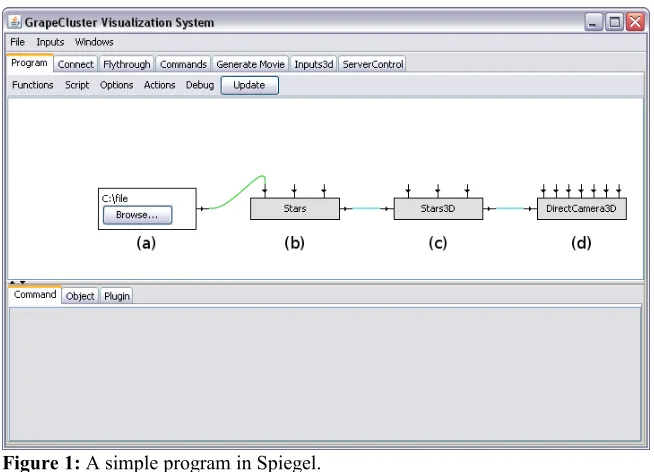
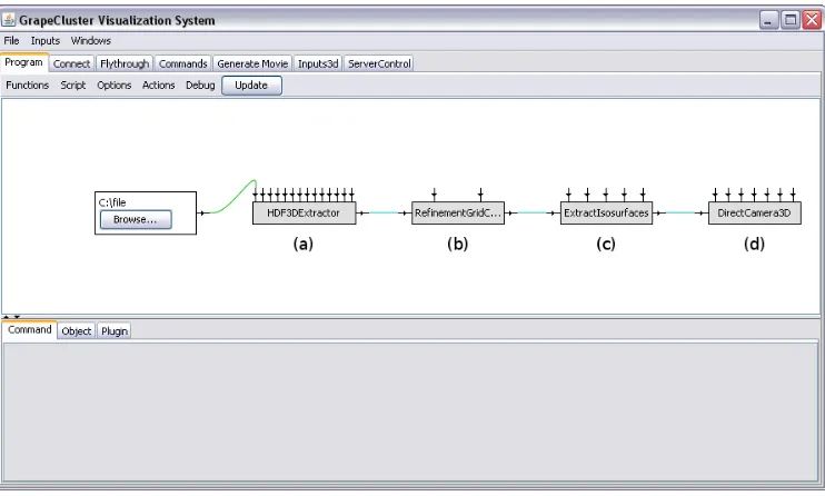
In Spiegel, programs are constructed by connecting task specific plugins together. Each

plugin can have zero or more inputs and outputs. A simple program that draws stars as individual 3D points is shown in figure 1. This particular program can be read from left to right as indicated by the labels in the figure. The file input plugin (figure 1a) allows the user to select a file in the local file system, which is passed as a string parameter to the star extractor plugin (figure 1b.) The star extractor plugin reads stars from the specified file and passes them as an input to the the Stars3D visualization plugin (figure 1c.) Stars3D converts the list of stars to a list of 3D points, which is then given as an input to a Java 3D camera (figure 1d.) Finally, the camera draws the points in an external window thereby producing a simple visualization of the stars contained within the file.

The new visualization plugins presented in this document behave in a way that is similar to the Stars3D plugin shown in figure 1c. That is, the new plugins will process data from some external source and then issue commands to a renderer to display images. Plugins are written as Java classes implementing interfaces that are specific to Spiegel.

4 New Classes

This section details the classes that were added to Spiegel. Package names are shown first followed by a list of classes that are new to the package.

● spiegel.viewcontrol.function.plugins.visual

TimeMeasure

● spiegel.viewcontrol.function.plugins.visual.isosurface

Cell

ExtractIsosurfaces FloatStack

MarchingCubes

RefinementGridConvert NOISE

StructuredGrid

● spiegel.viewcontrol.function.plugins.visual.pointCloud

Box

ColorFunction PointSearch ShrinkWrap TraceHeap TraceMinHeap TriangleBox

● spiegel.viewcontrol.function.plugins.visual.pointCloud.graph

TriGraph GraphCycle GraphSubdivide

● spiegel.viewcontrol.function.plugins.visual.stars

TimeSample WindowFunction

● spiegel.viewcontrol.function.plugins.visual.util

MaxHeap MinHeap Pair

Quickselect Quicksort Triple VArray

● spiegel.viewcontrol.function.plugins.input

DoubleToString

● spiegel.wm4 [22]

ApprPlaneFit3 Eigen

GMatrix GVector LinearSystem Matrix2 Matrix3 Matrix4 Plane3 Vector2 Vector3 Vector4 WMath

5 Visualization of Temporal Data

The TimeMeasure plugin is designed to track and visually summarize arbitrary object parameters as they vary over time. This visualization reuses some of Spiegel's existing functionality by representing objects with the Star class. The Star class presents itself as a relatively uncomplicated container for representing objects that can be modeled as points. Extractor plugins exist that read stars from different sources and output instances of the StarIDMap class, which represents a snapshot of every star in the simulation at a specific point in time.

The StarIDMap class is used to map unique identifiers to Star instances for the purpose of tracking individual stars throughout the simulation. This visualization uses each identifier to map Stars to windows, which store information about a Star's past and present values. The amount of data that a

window holds is determined by the visualization parameter windowSize.

5.1 Overview of Operation

Upon creation, each window uses a window function to allocate a total of windowSize

storage units. The set of all windows is associated with a single window function. A window does not make any assumptions about the contents of a storage unit; the window function is the only part of the visualization that knows what they actually contain. Each storage unit is initially considered to be "unassigned."

When an update occurs, a window is given a Star instance. The window uses the window

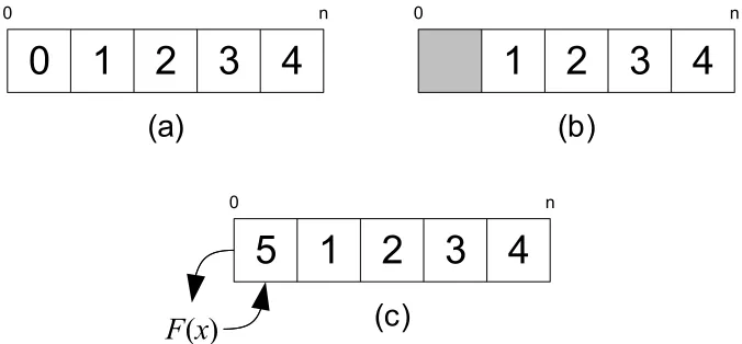
window will run out of unassigned storage units; when this occurs, the window will act like a LIFO buffer. The oldest assigned storage unit, the one with the minimum timestamp, will be marked as unassigned. The unassigned storage unit is reclaimed after the window function uses it to store the most recent data. (figure 2.)

Before an update ends, the window gives every assigned storage unit and their associated

timestamps to the window function as an Enumeration. The window function performs calculations on

the storage units and returns a single real value, which represents a summary of their contents. The meaning of the summary is completely dependent on the window function that is being used. The summary could, for example, represent a moving average of a Star's speed in inches per second. The window function provides a textual description of the calculations it performs, which is displayed to the user when the visualization is rendered.

After each window has been updated, the visualization will know the minimum and

maximum summary values for that update. The range of summary values that are discovered during an update is used to determine the range of summary values that should be displayed when drawing. The method used to determine the displayable range of values is controlled by the visualization's autoRange parameter.

5.2 TimeSample

The interface TimeSample in package spiegel.viewcontrol.function.plugins.visual.stars provides read only access to a container that associates a sample of type T with a timestamp. TimeSample only has two functions.

T getSample() double getTimestamp()

In the visualization, the getSample function always returns references to preallocated storage units. The getTimestamp function returns the time associated with the storage unit in seconds. Timestamps indicate the simulation time that the data in the storage unit originated from.

Figure 2: A window recycles storage units once all of them are in use. (a) A window with no inactive storage units. Each number represents an associated timestamp. (b) The oldest storage unit, the one with the minimum timestamp, is marked as inactive. (c) The inactive storage unit is reclaimed after window function F uses it to store the most recent data.

0 1 2 3 4

0 n

(a)

1 2 3 4

0 n

(b)

1 2 3 4

0 n

(c)

F

(

x

)

5.3 WindowFunction

The class WindowFunction in package spiegel.viewcontrol.function.plugins.visual.stars is the interface that the visualization uses to access window functions. A window function is responsible for creating, updating, and summarizing storage units of type T. The visualization treats storage units as containers for arbitrary data.

T createStorage()

The createStorage function is used to create a new storage unit instance. The choice of type T is completely decided by the class implementing the WindowFunction interface. A storage unit contains the values necessary for the window function to represent a Star for the purposes of the calculation it will perform. A class could, for example, choose to store direct copies of specific fields from the Star class in its storage units.

void copyToStorage(Star source, T dest)

The copyToStorage function is used by the visualization to copy a representation of source into the storage unit dest.

double summarize(Enumeration<TimeSample<T>> storage)

The summarize function is provided with an Enumeration of TimeSample instances that are used to associate timestamps with storage units. This function is expected to calculate a real value that represents a summary of the elements returned by the enumeration. The choice of the representation used to summarize the storage units is, again, completely decided by the implementing class. As an example, a class could use the summarize function to compute a moving average of a star's mass.

String getSummaryName()

The getSummaryName function is used to give the user a good idea as to what is actually

being visualized. The string returned by getSummaryName should contain a concise description of the

5.4 TimeMeasure

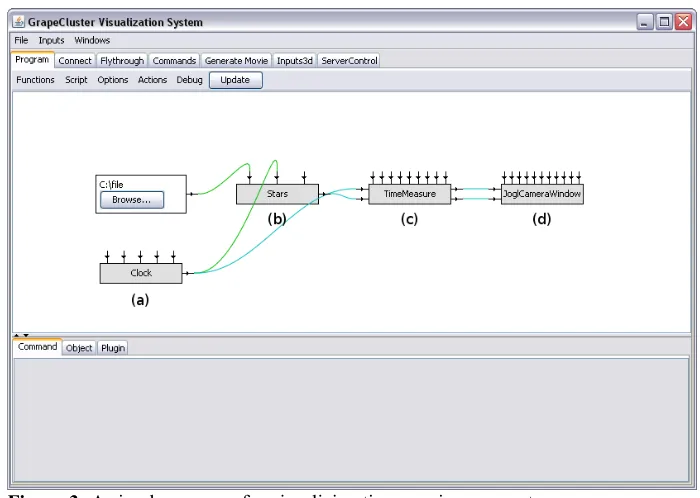
The TimeMeasure plugin in package spiegel.viewcontrol.function.plugins.visual implements the temporal visualization described throughout this section. Figure 3 shows a basic

Spiegel program that uses TimeMeasure. The Clock plugin (figure 3a) is used as the time source in this program. The outputs of Clock are connected as a parameter of Stars (figure 3b) and as one of the inputs to TimeMeasure (figure 3c.) This is an important detail as the value of the time parameter on the star extractor and the value of TimeMeasure's time input must be the same. The Stars plugin (figure 3b) was chosen as the star extractor for this example. Stars reads star data from a text file and outputs StarIDMap instances, which are given as the second input to TimeMeasure.

The TimeMeasure plugin has two outputs, both of which are connected to the inputs of the JOGL camera (figure 3d.) TimeMeasure's first output is an instance of a Drawable object, required to display the visualization. The second output is a list of annotations, which are optional but provide useful information about what the visualization is displaying.

5.4.1 Important Notes

A new TimeMeasure instance defaults to a "reset" state. During its first update after being reset, TimeMeasure allocates a window for each Star encountered in the StarIDMap given as an input. The time of each update is also recorded. After its initial update, TimeMeasure does not attempt to modify its windows if the time of the update is less than or equal to the time of the previous update. TimeMeasure only updates its storage when it detects that time is moving forward. Additionally, it is expected that each StarIDMap contains the same stars from the same simulation data that were present in the initial update.

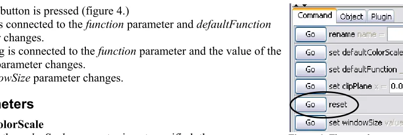
To correctly change the data source for the star extractor connected to TimeMeasure's input or to measure parts of the simulation beginning at an earlier time, TimeMeasure must be reset to its initial state. TimeMeasure's state is reset when any of the following events occur:

● The reset button is pressed (figure 4.)

● Nothing is connected to the function parameter and defaultFunction

parameter changes.

● Something is connected to the function parameter and the value of the

function parameter changes.

● The windowSize parameter changes.

5.4.2 Parameters

● defaultColorScale

When the colorScale parameter is not specified, the

defaultColorScale parameter chooses which of the predefined color scales to use. The choices are:

● Grayscale

A monochromatic color scale that linearly maps values to varying intensities of white. The lowest values are the least intense while the highest values are the most intense.

● HSV Scale

Linearly maps values to hues in the HSV color space. The lowest value

corresponds to the hue at 240º, a cool color, while the highest value corresponds to the hue at 0º, a warm color. Saturation and value are always set to their maximum values.

● defaultFunction

When the function parameter is not specified, the defaultFunction parameter chooses a predefined window function to use. The following functions are provided:

● Energy moving average

Calculates kinetic energy ( E=0.5mv2_{) [28] for each window entry then finds}

the average of all entries. This window function uses the mass and velocity fields of the Star class.

● Estimated speed moving average

Calculates speed as the magnitude of velocity [27] across pairs of entries then finds the average of all calculated speeds. The speed is said to be estimated since velocity is calculated using the Star class' position field instead of its velocity field. The position field contains the coordinates of a Star in world space.

● function

The function parameter is used to specify a custom window function. Instances of classes

implementing the WindowFunction interface are accepted.

● colorScale

The colorScale parameter is used to specify a custom color scale. Instances of classes implementing the ColorScale interface are accepted.

● windowSize

The windowSize parameter specifies the number of storage units that each window contains. The minimum value is 1.

● clipPlane

Specifies a plane that's used for clipping points when drawing. The values that define the plane's normal, x, y, and z do not need to be normalized. The clip plane is automatically disabled if the normal has a length of 0.

● enableClipPlane

When enableClipPlane is set to true, points that appear in front of the plane defined by the clipPlane parameter are not drawn.

● autoRange

After each update, the minimum and maximum window summary values are used to determine the range of values that should actually be displayed. When autoRange is set to false, a static range determination method is used. When autoRange is set to true, an automatic range determination method is used. The calculated display range affects how colors are chosen for each point. Points with summary values that are outside the display range are not drawn.

● Static method

The range of displayable values is set to the minimum and maximum summary values of the most recent update.

● Automatic method

The minimum and maximum summary values for the most recent update are stored as a range in an internal buffer. Up to x ranges are stored where x is

determined by the autoRangeSamples parameter. When the

autoRangeFilterOutliers parameter is set to false, the display range is

determined by finding the minimum and maximum values in the buffer. When the autoRangeFilterOutliers parameter is set to true, the display range is

determined by finding the medians of the minimum and maximum values in the buffer.

● autoRangeSamples

When autoRange is set to true, the autoRangeSamples parameter determines the total number of updates to consider when finding the minimum and maximum values of the display range. The minimum value is 1.

● autoRangeFilterOutliers

The autoRangeFilterOutliers parameter affects how the display range is chosen when autoRange is set to true. When autoRangeFilterOutliers is set to true, the display range's minimum and maximum values are equal to the medians of the minimum and maximum values of the stored ranges. When autoRangeFilterOutliers is set to false, the display range's minimum and maximum values are equal to the minimum and maximum values of the stored ranges.

● useTextures

When useTextures is set to false, points are drawn as plain untextured squares. When useTextures is set to true, points are drawn with blending enabled using a texture that fades around the edges. When textures are enabled, points are sorted based on their distance to the camera before they are drawn.

● pointSize

The pointSize parameter determines the size of the points that are drawn. The minimum value is 1.

6.1 Isosurfaces

Let Fx , y , z be a function that defines the values for a volume where x, y, and z represent coordinates within the volume. For simplicity, it will be assumed that F :ℝ3ℝ, or that F maps volume coordinates to real numbers. The values that volume coordinates are mapped to will be referred to as density values.

Suppose that points with a particular density are to be found. Given the equation

Fx , y , z−Iso=0 , where Iso, called the isovalue, is the value of the density to search for, a set of points can be obtained by solving this equation. Each point in the set corresponds to a point on one or more disjoint surfaces with the specified density value. Such surfaces are known as isosurfaces. [8] Additionally, the function F is known as the field function. [8] Finding isovalues in a volume is the definition of the isosurface extraction problem. [7]

6.2 Grids

A grid, in the context of the algorithms that will be discussed, is a division of 3D space using some geometric primitive. [9] Each primitive in the grid will be referred to as a cell. The

isosurface algorithms that will be examined either operate on a structured grid or an unstructured grid. A structured grid consists of cells that are either uniform or shape varying boxes. [10] Structured grids have the property that their cells can be directly addressed by indices. Because of this property, it should be clear that an array is one of the most obvious types of structured grids. Unlike structured grids, unstructured grids must store connectivity information cells in the grid. [9] The spatial

relationships between neighboring cells in an unstructured grid are not implicit as they would be in an array-like structure. [19]

Unless otherwise stated, when referring to a structured grid cell, the shape of that cell is a box. This is done to be consistent with the definitions found in the algorithms that will be presented in later subsections. Each cell has eight vertices and twelve edges, and each vertex is associated with a density value. A grid can be thought of as containing a set of unique density values that are associated with vertices from one or more cells.

6.2.1 StructuredGrid

The class StructuredGrid defines an interface that is used to allow the isosurface

visualization to operate on any type of three dimensional structured grid. The StructuredGrid interface only defines the functions that are necessary for solving the isosurface extraction problem as described in section 6.1. Included in the interface are functions for getting the dimensions of the grid along each axis, functions for getting the coordinates of an element at a specific index, and a function for getting the density value associated with an element at a specific index.

6.3 The Marching Cubes Algorithm

The Marching Cubes algorithm as defined in [6] describes a relatively simple method for isosurface extraction and triangulation that operates on structured grids. The two processes, isosurface extraction and triangulation, are integrated in this algorithm as a single pass over each cell in the grid. This algorithm treats each cell as an independent entity; the relation of a cell to its neighbors does not affect the resulting mesh of triangles.

An implementation of the Marching Cubes algorithm is provided by the MarchingCubes

class (section 6.3.2.) The MarchingCubes class uses the Cell interface (section 6.3.1) to represent different portions of a structured grid. The rest of this section describes how the Marching Cubes algorithm detects intersections in individual cells and generates triangles to represent those surfaces.

The vertex of each cell in a grid was previously defined as being associated with a density value. For the Marching Cubes algorithm, a cell's vertices are given an additional property: each vertex will be associated with a boolean flag. The state of this flag is determined by a vertex's associated density value. A vertex's flag is set to true if its associated density value is greater than or equal to the isovalue, otherwise the flag is set to false. Having a flag value of true implies that a vertex is either inside the isosurface or directly on its perimeter.

An intersection between a cell and an isosurface is detected by examining the state of each vertex's flag. If one of the cell's edges has, for example, a vertex with a flag set to true at one endpoint and a vertex with a flag set to false at the other endpoint, it should be apparent that the isosurface intersects the edge at some point. Edge intersections are used to infer the structure of an isosurface.

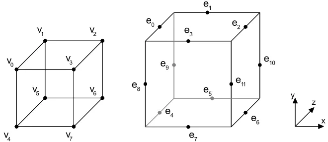
The representation that will be used for a cell in this section and in the MarchingCubes class is based on the representation in [6] as shown in figure 5.

Since each vertex is associated with a flag that can take on one of two states, each cell can be viewed as having a total of 28_{, or 256, possible states. The paper takes advantage of a cell's}

symmetry when its center is positioned at the origin to define 14 unique states. This smaller set of states can be used to derive the 256 cell states by, again, using the symmetric properties of a cell. The paper does this reduction to make the creation of a table that stores information for each cell state less tedious and error prone.

Since the flag associated with each vertex in a cell encodes one of two states, an index to the table of cell states can be created by assigning the value of each vertex flag to a bit in an 8-bit integer. Following the paper's definition of an index, for each vertex, vi, where i∈{0, 1, 2, 3, 4, 5,6, 7},

Figure 5: The arrangement of cell vertices and edges used by the MarchingCubes class. Left: Cell vertices. Right: Cell edges.

e₀ e₁ e₂ e₃ e₄ e₅ e₆ e₇

e₉ e10

e₁₁ v₀

v₁ v₂

v₃

v₄

v₅ v₆

v₇

e₈

the value of bit i in the index is 1 if the flag for vi is true or 0 if the flag for vi is false. Each entry in the

table of cell states includes a list that identifies the edges in the cell that have been intersected. The table used by the MarchingCubes class stores a variable length list for each state. Each list contains zero or more references to edges that have been intersected. The edges are arranged in groups of three so that their points of intersection can be used to directly create the triangles that represent the

intersecting isosurface. Every cell that is intersected by the isosurface will have a minimum of three intersected edges.

Given a set of edges in a cell that have been intersected by an isosurface, the points of intersection can be determined as follows. As mentioned earlier, each cell edge that is identified as having been intersected will have one vertex that's on or inside the isosurface and one vertex that's outside the isosurface. By taking the density values associated with a pair of vertices of an edge, the point of intersection can be obtained by using linear interpolation to determine which point on the edge would correspond to the isovalue.

To find the normal at the point of intersection on an edge, the normals for the edge's

endpoints must first be calculated. Normals for each cell vertex are calculated through the estimation of gradients as shown by the equations in [6]. The normal for the point of intersection is obtained by linearly interpolating the normals of the endpoints along the edge to the location of the intersection and normalizing the result.

6.3.1 Cell

The Cell class defines an interface for accessing a generic cell. The interface itself doesn't impose any specific requirements for the structure of a cell. The following functions are defined:

int getNumVertices()

Determines the number of vertices the cell contains. Valid vertex indices are in the range of [0, getNumVertices()).

Vector3f getNormal(int vertex)

Calculates the normal of a vertex.

double getValue(int vertex)

Gets the density value associated with a vertex.

Tuple3d getPoint(int vertex)

Gets the position of a vertex in world space.

6.3.2 MarchingCubes

The MarchingCubes class contains an implementation of the Marching Cubes algorithm and provides two main features - the ability to divide a StructuredGrid into a set of cells for

enumeration and the extraction of intersecting isosurfaces from individual cells. The MarchingCubes

class has minimum dimensionality requirements for the structured grids that it operates on. The grid must contain enough data to represent a single cell, which corresponds to a grid having a length of 2 on all axes. Construction will fail unless a grid is compatible. To check the compatibility of a grid, the static function isGridCompatible can be used.

If isGridCompatible returns true then construction of a new MarchingCubes instance can proceed.

MarchingCubes(StructuredGrid grid)

After construction, access to the cells implicitly created by the StructuredGrid is required to perform isosurface extraction. There are two functions in the MarchingCubes class that provide

information relating to the cells it contains.

int getNumCells()

Enumeration<Cell> getCellEnumerator()

The getNumCells function returns the total number of cells created by the grid and the getCellEnumerator function gets a new Enumeration that enumerates every cell in no particular order. Because of the requirements imposed by the constructor, there will always be at least one cell available. To perform operations on a cell, the function extractSurface is used.

void extractSurface(Cell cell, double isovalue, FloatStack pointsOut, FloatStack normalsOut)

Given a cell, extractSurface tests for the intersection of an isosurface with the specified isovalue. If the cell is intersected by an isosurface then triangle positions and normals are calculated and stored in pointsOut and normalsOut. The positions and normals for each triangle vertex are specified as groups of three values corresponding to the axes in this order: x, y, and z. normalsOut can be null if the calculation of normals are not required.

6.4 A Near Optimal Isosurface Extraction Algorithm Using the Span Space

(NOISE)

Unlike the Marching Cubes algorithm, the approach taken by the algorithm in [7] can operate on both structured and unstructured grids. This algorithm introduces the concept of a span space, which requires a preprocessing step to construct, but is intended to accelerate the process of isosurface extraction.

The NOISE algorithm associates a pair of values with each cell that represent the minimum and maximum density values of a cell's vertices. The span space consists of minimum and maximum value pairs from every cell in the grid. The span space is, therefore, two dimensional. As the paper points out, the Marching Cube algorithm searches a three dimensional space of points to find

isosurfaces. By utilizing the span space for isosurface extraction, the search space is reduced from three to two dimensions. The span space also provides a method for culling unwanted cells, which are cells that are not intersected by an isosurface.

partitioned into two smaller sets, the first subset contains all cells that have a value that is less than the median, and the other set contains all cells that have a value that's greater than or equal to the median. The cell with the median is stored in the node and construction continues when the subsets are passed to the children. Note that at each level in the tree, the next value in the pair will be examined. For example, if the median was chosen from the minimum values at level 0 in the tree then at level 1, the median is chosen from the maximum values and so on.

The construction of the tree can be done with a running time of O(k log2k), where k is

equal to the total number of cells in the grid. This running time can only be achieved if the selection of the median can be done in O(n) steps. The paper uses the selection algorithm described in [20], which is sometimes called quickselect. The claim is that the quickselect algorithm has an average case running time of O(n) with randomly chosen pivots. [7] [21]

The paper states that the worst case running time for finding every cell that is intersected by an isosurface is O



The triangulation of cells from an unstructured grid is also discussed in the paper, but what's more interesting is now that a fast method for extracting isosurfaces has been developed, other methods for creating triangles from the intersected cells of structured grids can be substituted at this point. In particular, the Marching Cubes algorithm could be used to extract isosurfaces from each intersected cell as they are discovered.

6.4.1 NOISE

The NOISE class contains an implementation of the NOISE algorithm. It uses an existing instance of the MarchingCubes class to get a cell based representation of a grid.

NOISE(MarchingCubes cubes)

When a new NOISE instance is created, a tree containing every cell returned from cube's enumeration is constructed. A reference to cubes is stored that is later used when extracting isosurfaces.

void extract(double isovalues[], FloatStack points, FloatStack normals)

6.5 ExtractIsosurfaces

The ExtractIsosurfaces plugin combines the algorithms and classes described in this section to produce an isosurface visualization. Figure 6 shows a basic Spiegel program for visualizing

isosurfaces. In this program, volume data is loaded from a file and stored in a RefinementGrid (figure 6a.) A subgrid is extracted from the RefinementGrid and placed in a StructuredGrid wrapper (figure 6b.) The StructuredGrid is given as an input to an instance of ExtractIsosurfaces (figure 6c), which compiles a list of triangles that are sent to the Java 3D camera (figure 6d) for display.

6.5.1 Parameters

● isovalues

The isovalues parameter takes a string containing one or more real numbers separated by commas. An isosurface is extracted for each isovalue that is specified. Avoid entering the same isovalue multiple times; the visualization does not check for duplicate isovalues.

● useNOISE

When useNOISE is set to false, the visualization uses the Marching Cubes method of

isosurface extraction. That is, every cell from the grid is examined while searching for intersected cells.

When useNOISE is set to true, a tree containing every cell from the grid is constructed whenever the input grid changes as described by the NOISE algorithm. The tree is used to reduce the number of cells that are examined when extracting isosurfaces, potentially improving performance. It is usually safe to enable this feature when the input grid doesn't change or changes infrequently and one or more isosurfaces are extracted across multiple updates. Enabling this feature in most other situations could cause a decrease in

performance due to the overhead associated with constructing the tree.

● wireframe

When the wireframe parameter is set to true, only the edges of the output triangles are drawn.

● cull

When the cull parameter is set to true, triangles from the output are only drawn if they are facing the camera. When the cull parameter is set to false, every triangle from the output is drawn regardless of their orientation.

● material

The material parameter is used to associate a custom material with the output triangles. If a material is specified for this parameter, lights must be added to the scene for the output triangles to be visible. If nothing is specified for this parameter, the visualization uses a default material that ignores lighting.

7 Surface Reconstruction From a Set of Points

Given an unorganized set of points, which will be referred to as a point cloud, the goal is to generate a closed surface represented by a mesh of triangles that closely approximates the overall shape of the cloud. This task is a type of surface reconstruction problem which, in general, can be described as the process of finding a surface that approximates some unknown surface defined by a finite set of discrete samples. [13] [17]

One simplifying assumption that will be made is that every point cloud is noise free. That is, any point cloud provided by a user is assumed to represent the near exact shape of the unknown

surface. The process described in Direct Reconstruction of a Displaced Subdivision Surface From

Unorganized Points [12] will be implemented to create surfaces for this visualization. Surface construction proceeds in four major steps, with each step providing a greater refinement of the approximated surface over previous steps.

For the first part, a mesh is generated in the form of a subdivided box that surrounds the point cloud. The nodes of the mesh are modified through a "shrink wrapping" process, which moves the nodes of the box closer to the points in the point cloud over several passes. Shrink wrapping produces a fairly good initial approximation of the point cloud's shape. The second part involves mesh simplification to create a coarse control mesh; the mesh is simplified as much as possible without changing its overall shape. The third part subdivides the control mesh to create a smooth domain surface. [18] Finally, points in the point cloud are used to approximate the shape of the local surface of the cloud itself near parts of the domain surface. The domain surface's nodes are then displaced so that its shape closely matches the shape of the surfaces found in the point cloud.

Unless stated otherwise, classes referred to in this section can be found in the package spiegel.viewcontrol.function.plugins.visual.pointCloud. The surface reconstruction process that is described focuses on manipulating a mesh of triangles; the mesh in the visualization is represented by a graph. The graph and its related classes are described in section 8.

7.1 Shrink Wrapping

The first step in the surface reconstruction process involves finding an initial approximation of the point cloud's shape using a method known as shrink wrapping. The general idea of shrink

wrapping involves generating a mesh that completely encircles the point cloud then, over several iterations, moving each node in the mesh towards nearby points in the cloud while attempting to maintain a fairly even distribution of nodes across the entire mesh.

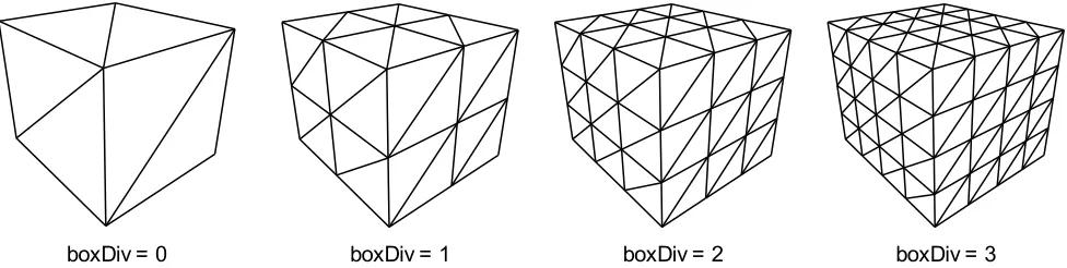
static TriGraph create(Tuple3d min, Tuple3d max, final int edgeDiv) throws RuntimeException

The bounds of the box are stored in min and max. The edgeDiv argument specifies the number of times to divide each of the box's edges. The minimum valid value for edgeDiv is 0, which results in a plain bounding box. Using higher values for edgeDiv can creates boxes that have more points distributed across their surface. When the create function is called by the visualization, it uses the value of its boxDiv parameter (section 7.5) as the value for the edgeDiv argument. Figure 7 shows how the choice of the value for boxDiv affects the overall distribution of points on the subdivided box that is generated.

After the initial mesh has been created, shrink wrapping is performed to wrap the mesh around the point cloud. Shrink wrapping is an iterative process that performs two operations on the mesh during each pass. These operations are referred to as projection and smoothing in [12].

7.1.1 Projection Operator

The projection operator applies an "attracting force" to each node in the mesh, moving them closer to the point cloud. For each node, a point closest to the node's current position is located in the point cloud. An attracting force vector is calculated by taking the closest point's position and subtracting it by the node's position. This difference is then scaled by the projection speed, which is a constant in the range of (0, 1). The attracting force is applied to the node by adding the scaled

difference to the node's position.

/* Projection operator */ for each node in mesh {

Vector closest = find point in point cloud closest to node.position; Vector force = (closest - node.position) * projectionSpeed;

node.position += force; }

The closest points in the point cloud are found using the PointSearch class, which contains an implementation of the kd-tree based algorithm from [15] that can locate the closest n-dimensional records to a target in logarithmic expected time. The projection speed for the visualization is controlled

Figure 7: The value chosen for the boxDiv parameter affects the total number of nodes present on the surface of the subdivided box used for shrink wrapping.

by the projectSpeed parameter.

7.1.2 Smoothing Operator

The smoothing operator displaces node positions with the intention of creating a somewhat more uniform distribution of nodes across the mesh; it is based on some of the concepts presented in [23]. The smoothing operator begins by finding the approximate Laplacian of the node, which is equal to the average of the sum of differences in positions between each of the node's neighbors and the node itself. The tangential Laplacian, which is perpendicular to the node's normal, is calculated using the approximate Laplacian. The tangential Laplacian is then scaled by constant in the range of [0, 1], known as the smoothing speed, and summed with the node's position to displace the node.

/* Smoothing operator */ for each node in mesh {

/* Compute approximate Laplacian */ Vector laplacian = Vector(0, 0, 0); int totalNeighbors = 0;

for each neighbor of node {

laplacian += neighbor.position - node.position; totalNeighbors++;

}

laplacian /= totalNeighbors;

/* Compute the tangential Laplacian */

Vector tangent = laplacian - dotProduct(laplacian, node.normal) * node.normal;

/* Scale the tangential Laplacian by the smoothing speed */ tangent *= smoothingSpeed;

/* Displace the current node */ node.position += tangent;

}

The value used for the smoothing speed by the visualization is determined by the smoothSpeed parameter.

7.2 Mesh Simplification

After shrink wrapping completes, the mesh should represent a reasonable approximation of the point cloud's shape. This part of the surface reconstruction process involves simplifying the shrink wrapped mesh to produce a much coarser mesh. The coarse mesh will be used as a control mesh in the

next part to create a smooth domain surface. The algorithm presented in Surface Simplification Using

Quadric Error Metrics [14], referred to as the QEM algorithm, is used to simplify the shrink wrapped mesh.

7.2.1 Fundamental Error Quadrics

the mesh. The fundamental error quadric, Kp, as with all other error quadrics, is a symmetric 4x4

matrix. Kp is defined as:

Kp=

[

a2 ab ac ad ab b2 bc bd ac bc c2 _cd

ad bd cd d2

]

The subscript p refers to the plane of the triangle whose fundamental error quadric is being calculated. a, b, and c are equal to the x, y, and z coordinates of the plane's normal and d is equal to the plane's distance from the origin. The values chosen for a, b, c, and d must satisfy the equations ax + by + cz + d = 0 and a2 _{+ b}2 _{+ c}2 _{= 1. The coordinates of the position of any triangle node can be substituted}

for x, y, and z in the first equation.

In [12], the fundamental error quadrics are based off of planes found from points in the point cloud instead of the triangles from the mesh. Let r be a point from the point cloud. To calculate a plane for r, its neighborhood must be found. The neighborhood of r is the set of all points from the point cloud whose distance from r is less than θ. The plane used for r is equal to a plane that fits r's neighborhood. The ApprPlaneFit3 class in the package spiegel.wm4 contains algorithms to fit a plane to a set of points using the least squares method. After finding a point's plane and associated

fundamental error quadric, it is projected onto one of the mesh's triangles. Once all points have been projected, a triangle's fundamental error quadric is equal to the sum of the fundamental error quadrics of the points that have been projected onto it.

There are several issues with basing the calculations of the fundamental error quadrics on the point cloud. The first issue is that the user is expected to choose a good value for θ, the search radius used to find neighborhoods in the point cloud.Ideally, the value chosen for θ will find neighborhoods that are a good approximation of the surface around most points. There isn't a particularly good default value for θ since the outcome of a neighborhood search is completely dependent on the arrangement of points in the point cloud.

Another issue is that it was not possible to create an algorithm for projecting points onto a mesh with a reasonable running time. Other than stating the goal of the problem, no insight was given as to what method was used in [12]. Because of these problems, the visualization uses the unmodified QEM algorithm. The visualization does not use the point cloud when calculating the fundamental error quadrics for the triangles. It is shown in [12] that basing the calculation of the fundamental error quadrics on the point cloud can lead to a more accurate representation of the point cloud's shape in the simplified mesh. Hopefully the time saved by not doing the projections or manually searching for a good value for θ outweighs the cost of potentially having slight inaccuracies in the control mesh.

7.2.2 Initial Error Quadrics

An initial error quadric is computed for each node in the mesh. A node's initial error quadric is equal to the sum of the error quadrics of every triangle that uses the node. When using the graph to represent the mesh, the triangles that reference a node can be found with the node's

getTriangleEnumerator function (section 8.1.1.)

7.2.3 Edge Heap

collapsing. An edge can only be added to the heap after its error quadric and point of contraction are found. The error quadric for an edge is equal to the sum of the error quadrics of its endpoints. The point of contraction for an edge can be found by first constructing a matrix, I.

I=

[

Q_0,0 Q_0,1 Q_0,2 Q_0,3 Q_0,1 Q_1,1 Q_1,2 Q_1,3 Q0,2 Q1,2 Q2,2 Q2,3

0 0 0 1

]

Q is the edge's error quadric and Qy,x refers to the element at row y, column x in Q. If matrix

I is invertible, then the point of contraction v' is calculated as shown below.

v '=I−1

[

]

If matrix I is not invertible, then [14] recommends choosing one of three points from the edge as the point of contraction - either one of its endpoints or its midpoint. For simplicity, an edge's midpoint is always chosen as the point to use for v' when I is found to not be invertible. In this case, the value of v' is equal to the average of the positions of the edge's endpoints.

An edge's error quadric and its point of contraction are used with the error function to find the cost of collapsing the edge.

errorQ , x , y , z=x2_Q

0,02xy Q0,12xz Q0,22x Q0,3y 2_Q

1,1

2yz Q1,22y Q1,3z2Q2,22z Q2,3Q3,3

The error function computes a scalar that represents the error of point x, y, z with respect to error quadric Q. Edges are added to the heap keyed by their cost once their point of contraction has been found. Mesh simplification begins after every edge has been added to the heap.

7.2.4 Edge Collapsing

Mesh simplification is an iterative process that begins by removing the edge that's at the top of the edge heap. Since the graph's edge collapsing function will be used, a replacement node is created that has the same position as the edge's point of contraction. The graph function collapseEdge is called using the edge and replacement node as arguments.

After the edge is collapsed, the replacement node will contain edges that connect it to the nodes that were originally neighbors of the edge's endpoints. Before updating the edges that connect the replacement node to its neighbors, the error quadric for the replacement node must be set to the error quadric that was associated with the collapsed edge.

After the affected edges in the heap are updated, simplification can continue as described at the beginning of this section. Simplification continues until some desired number of nodes, triangles, or edges are reached. The visualization uses a termination condition that is similar to the one used in [12];

mesh simplification ends when the number of nodes that would result from subdividing the graph x

times is approximately equal to the number of points in the point cloud. The value of x is adjustable by the user as described in section 7.5.

7.3 Subdivision

The simplified mesh is used as the control mesh for the subdivision algorithm. To perform subdivision, the visualization uses the GraphSubdivide class (section 8.3), which contains an

implementation of Loop's subdivision algorithm. [16] Because Loop's subdivision algorithm causes shrinkage in the output mesh, the positions of the control mesh's nodes are displaced before

subdividing to minimize the effect.

7.3.1 Control Mesh Correction

Each node in the control mesh has an explicit representation on the subdivided surface. To find this representation, a node's limiting position is calculated. The function getLimitingPosition in GraphSubdivide can be used to calculate a node's limiting position. Using the limiting position, the closest point in the point cloud is found. The resultant force, ri, is calculated as in [12] and then scaled

by the displacement speed, a constant in the range of [0, 1]. The displacement speed in the visualization is determined by the controlSpeed parameter. A node is displaced by adding ri to its position.

After displacing every node in the control mesh, the closeness of the limiting positions to the point cloud is evaluated with the error energy function defined in [24]. The error energy function is equal to the average distance between each limiting position and the point closest to it in the point cloud. Node displacement repeats until the energy falls below a certain threshold, set by the visualization parameter energyTarget.

7.3.2 Control Mesh Subdivision

The corrected control mesh is subdivided one or more times using the subdivide function in GraphSubdivide. As described in section 7.5, the number of times that the control mesh is subdivided can either be determined automatically or manually specified by the user.

7.4 Surface Detail Sampling

7.5 ShrinkWrap

A simple surface reconstruction program is shown in figure 8. The VectorOf3dPointE

plugin (figure 8a) reads point data from specially formatted files and outputs instances of the VectorOf3dPoints class. The output from the VectorOf3dPointE plugin is given as the input to the ShrinkWrap plugin (figure 8b.) The ShrinkWrap plugin generates a mesh using the surface

reconstruction process described in this section and outputs a set of triangles. The triangles output by the ShrinkWrap plugin are given as an input to a Java 3D camera (figure 8c), which displays them to the user.

7.5.1 Parameters

● mode

The mode parameter sets the mode of operation for the visualization.

● Mode 0: Point cloud (debug)

Outputs a group of points for display based on the input points. The points are colored with a shade of pink and are not affected by lights in the scene.

● Mode 1: Shrink wrap (debug)

Only performs shrink wrapping on the mesh. The output contains the point cloud and the shrink wrapped mesh drawn in wireframe mode. Lighting is disabled for the material that's used with the mesh.

● Mode 2: Control mesh (debug)

Performs shrink wrapping, simplification, and control mesh correction. The output contains the point cloud and the control mesh drawn in wireframe mode. Lighting is disabled for the material that's used with the mesh.

● Mode 3: Shrink wrap only

Only performs shrink wrapping on the mesh. The output contains the shrink wrapped mesh without any special modifications to its parameters.

Mode 4: Shrink wrap and subdivide

Performs shrink wrapping, simplification, control mesh correction, and subdivision. The output contains the subdivided mesh without any special modifications to its parameters.

● boxDiv

Determines the number of times each edge the box used for shrink wrapping is divided. Increasing the value of boxDiv increases the number of nodes that are distributed across the surface of the box as described in section 7.1. The value chosen for boxDiv can affect the overall quality of the approximated point cloud shape found through shrink wrapping. The default value for boxDiv is 8, which is usually a good starting point. The minimum value for boxDiv is 0.

● shrinkSteps

The shrinkSteps parameter determines the number of times that the projection and smoothing operators are applied during the shrink wrapping process. Using a value for shrinkSteps that's different from its default might require changes to the projectSpeed and smoothSpeed parameters. The minimum value for shrinkSteps is 0, which effectively disables shrink wrapping.

● projectSpeed

The projectSpeed parameter controls the speed of the projection operator that's used during shrink wrapping. Valid values for projectSpeed are in the range of (0, 1). Choosing a value

that's very close to projectSpeed's minimum or maximum values is not recommended.

Choosing a value that's too low will cause the mesh to move towards the point cloud too slowly. Choosing a value that's too high will cause the mesh to move towards the point cloud too quickly, potentially causing multiple nodes to converge at similar points. The default value is 0.5, which should work well in most situations.

● smoothSpeed

The smoothSpeed parameter controls the speed of the smoothing operator that's used during shrink wrapping. Valid values for smoothSpeed are in the range of [0, 1]. Lower values "relax" the mesh more, causing nodes to spread further from each other. Higher values reduce the relaxing effect. The default value for smoothSpeed is 0.8.

● controlSpeed

The controlSpeed parameter determines the speed of node displacement during control mesh correction. Valid values for controlSpeed are in the range of [0, 1]. The default value of 0.8 should work well in most situations.

● energyTarget

The energyTarget parameter sets the desired value for the average distance between the limiting positions of nodes and the position of their "ideal" point from the point cloud. The minimum value for energyTarget is 10-6_{. The value that is chosen for energyTarget affects}

the number of iterations required during control mesh correction. Choosing a value that's very low might not only cause an excessive number of iterations but could also cause nodes to converge too closely to each other. The default value for energyTarget is 10-2_.

● autoSubdiv

Let x be the total number of points in the point cloud. subdivision levels = 1 if x1000

subdivision levels = 2 if 1000≤x8000 subdivision levels = 3 if 8000≤x50000 subdivision levels = 4 if x≥50000

The choice of the values presented above is based on the observation that the number of nodes, edges, and triangles in the graph increases exponentially across multiple

subdivisions. Since the simplification process bases its stop condition on the number of subdivisions that will be performed and the number of points in the point cloud, choosing an inappropriate number of subdivisions could cause oversimplification of the mesh.

● subdivLevels

When the autoSubdiv parameter is set to false, the subdivLevels parameter determines the total number of subdivisions to perform on the control mesh. As explained for the

autoSubdiv parameter, the number of subdivisions affects the total amount of simplification

performed when creating the control mesh. The minimum value for subdivLevels is 1.

Setting subdivLevels higher than 4 is not recommended.

● wireframe

When the wireframe parameter is set to true, only the edges of the output triangles are drawn. Lighting for the material associated with the output triangles is disabled when wireframe is set to true.

● cull

When the cull parameter is set to true, triangles from the output are not drawn if they are not facing the camera when the scene is rendered. When the cull parameter is set to false, triangles from the output are always drawn regardless of their orientation.

● showPoints

Setting showPoints to true causes the visualization to display every point from the input. Certain visualization modes automatically set showPoints to true.

● material

The material parameter can be used to set a custom material that is associated with any triangles that the visualization outputs. When a material is specified, lights must be added to the scene to see the output of certain modes. If a value for the material parameter is not specified, the visualization uses a default material that ignores any lights in the scene.

● vertexColorFunction

The vertexColorFunction parameter accepts instances of classes implementing the

ColorFunction interface. When a vertex color function is specified, the color of each vertex in the output mesh is determined by the color function instead of the material.

● debugMessages

When the debugMessages parameter is set to true, messages are sent to the console that describe the output generated by the various steps of the surface reconstruction process.

8 Graph Classes

8.1 TriGraph

The TriGraph classprovides the ability to create and modify a graph based representation of a triangle mesh. Each graph contains three main components: nodes, edges, and triangles.

8.1.1 TriGraph.Node

Each node in the graph represents a triangle vertex and has three publicly accessible variables:

final Point3d pos final Vector3d normal final int id

The position of the node is stored in pos and the normal of the node is stored in normal. The constant id represents a numeric identifier that is used to distinguish each node in the graph. More information on identifiers can be found in section 8.1.4.

Internally, each node contains lists of each edge and triangle that it is associated with; these lists are automatically modified by the graph as it changes. Associations with other components of the graph can be queried either directly or indirectly. To enumerate every component that the node is

associated with, the functions getEdgeEnumerator and getTriangleEnumerator can be used.

Enumeration<Edge> getEdgeEnumerator() Enumeration<Triangle> getTriangleEnumerator()

Each edge returned by the edge enumerator has the property that the start node is equal to the node whose edges are being enumerated and the end node is equal to one of the node's neighbors. The start and end nodes of an edge never reference the same node. Other functions for querying a node's neighbors include:

boolean hasNeighbor(Node which)

Determines if a node has a specific neighbor.

Edge getEdge(Node toNode) throws RuntimeException

Assuming toNode is a neighbor of the node for which this function is invoked, an edge from the node's list of edges is returned that has toNode as its end node. An exception is thrown if toNode does not exist as a neighbor.

int getNumNeighbors()

Gets the total number of neighbors that a node has.

A function, boolean isReferenced(), is also provided to determine if a node is being

used in any part of the graph. isReferenced returns true if a node's list of edges or triangles are not empty.

8.1.2 TriGraph.Edge

final int id

The id constant represents an edge's identifier. Identifiers and their usage are explained in section 8.1.4. Edges cannot be directly modified as their public functions provide read only access to their contents.

Node getStart()

Gets the first node that represents one of the edge's endpoints.

Node getEnd()

Gets the second node that represents one of the edge's endpoints.

boolean isValid()

Determines if this edge is valid. Edges are invalidated when they are removed from the graph. Edges should only be checked for validity before use when holding references to edges across modifications to the graph.

8.1.3 TriGraph.Triangle

Triangles represent a cycle in the graph that is composed of three nodes. Triangles

implicitly show a relationship between three nodes; this same relationship is shown explicitly through edges, which are added to the graph if they do not already exist at the time the triangle is created. Triangles expose three publicly accessible variables:

final Vector3d normal final Plane3d plane final int id

The variable plane represents the plane formed by the triangle's three nodes. The variable normal contains the triangle's surface normal, which is a direct copy of the normal from plane. When a triangle is first created, the normal and plane variables are set to some arbitrary state and are

considered to contain invalid values until the graph's normals are calculated (section 8.1.5.) The constant id is the triangle's identifier. The use of identifiers is explained in section 8.1.4.

Each node of a triangle is usually referred to as a vertex. Triangle vertices can be accessed through the getVertex function.

Node getVertex(int i)

The getVertex function takes a single argument that represents the index of the vertex to get. Valid values for this argument are either 0, 1, or 2. The vertices returned from the getVertex

function also reveals their relationship with each other. For vertex vi = getVertex(i), there exists an edge

between vi and v(i+1) mod 3 where i∈{0, 1, 2}.

Triangles also have the ability to detect if a point is potentially inside of them. A point is inside of a triangle if it lies on its surface and is within the boundaries defined by its edges. The

function pointInside determines if a point is within a triangle's boundaries without requiring the point to be on the plane defined by the triangle's vertices.

pointInside only works correctly if the variables normal and plane reflect the current state of the triangle, which, as stated earlier, are updated whenever the graph's normals are calculated. To determine if a point is within the boundaries of a triangle, the point is tested against planes that are created for each of the triangle's edges as shown in figure 9.

For each edge in the triangle, a plane is created that is perpendicular to the triangle's

surface. An edge lies on the plane it is associated with. Each plane's normal points towards the inside of the triangle. A point is considered to be within the triangle's boundaries if it is either in front of or on each of the three planes.

Any point within the boundaries of triangle does not necessarily represent a point that's actually part of the triangle. A point that was tested and found to be within the triangle's boundaries must be projected onto the triangle's plane to get a point that's on the triangle's surface.

The final function of interest is the isValid function:

boolean isValid()

The isValid function for a triangle has the same usage as the isValid function for an edge. Triangle validity only needs to be tested before using any of its other functions when attempting to access references to triangles being held across modifications to the graph.

8.1.4 Numeric Identifiers

Each graph component - nodes, triangles, and edges - contains a public variable named id, known as the component's identifier. The primary function of an identifier is to distinguish each component within a set of components of the same type. Identifiers can also be used as indices to arrays to locate graph components in constant time. Information about the range of values used by the

identifier of each component can be obtained using the getMaxNodeID, getMaxTriangleID, or

getMaxEdgeID functions described in section 8.1.7.

8.1.5 Graph Creation

After a new instance of TriGraph has been created, at least three nodes must be added to

Figure 9:Left: A triangle. Right: The three planes created for the triangle's edges that are perpendicular to the triangle's surface. The arrows show the direction of each plane's normal.

v₁

v₀ v₂

y x

the graph before any other components can be created. Nodes are created with the addNode functions.

Node addNode(double x, double y, double z) Node addNode(Tuple3d point)

Both functions perform the same action - a new node with the specified coordinates is added to the graph then a reference to the new node is returned. The graph does not perform any checks to ensure that no two nodes are created with the same position; this is a task that is left to the user of the graph. Duplicate nodes can be created, but doing so is generally considered undesirable.

It is possible to store node identifiers instead of references to the nodes themselves. Nodes can be retrieved if their identifier is known using the getNode function.

Node getNode(int id) throws RuntimeException

getNode returns a reference to the node with an identifier of id. An exception is thrown if id is not a valid identifier. Although it is possible to access every node in the graph through this function, getNode should not be used for the enumeration of nodes; component enumerators are described in section 8.1.7.

After obtaining references to at several nodes, triangles can be created with the addTriangle function.

void addTriangle(Node n1, Node n2, Node n3) throws RuntimeException

addTriangle takes three nodes as arguments. Every node passed to this function must be unique otherwise an exception is thrown. The arguments specify the exact order of the triangle's vertices; n1 = vertex0, n2 = vertex1, and n3 = vertex2. Edges, if they do not already exist, are added

between the pairs of nodes (n1, n2), (n2, n3), and (n3, n1). Although the graph avoids creating duplicate

edges, it does not perform any checks to prevent the creation of duplicate triangles. Calling addTriangle with the same arguments more than once should be avoided.

The TriGraph.Node and TriGraph.Triangle classes contain variables whose values are not computed unless requested. These variables are normal in TriGraph.Node and plane and normal in TriGraph.Triangle. A request for the computation of these variables is made using TriGraph's calcNormals function.

void calcNormals()

calcNormals performs calculations on every node and triangle in the graph. It is important to remember to call this function after modifying the graph if access to the correct values of the previously mentioned variables is required.

8.1.6 Graph Manipulation

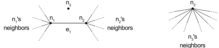
A single function is provided for removing edges from the graph by "collapsing" them.

void collapseEdge(Edge collapse, Node replacement) throws IllegalArgumentException, RuntimeException

and replacement, which represents the point of contraction for the collapsed edge. The general collapsing procedure is shown in figure 10.

An edge is collapsed by replacing all references to its two end points with the replacement node and then removing the edge and its endpoints from the graph. The node that is passed to

collapseEdge as the replacement node must not be used in any part of the graph (checked with TriGraph.Node's isReferenced function) otherwise an exception is thrown. When an edge is successfully collapsed by collapseEdge the following is true:

● collapse will have been removed from the graph and invalidated

● Any triangle that uses both of collapse's endpoints is removed from the graph and invalidated

● The endpoints of collapse will not be used by any other component in the graph

● The edges that previously connected the endpoints to their neighbors will be modified so that

these edges are connected to replacement instead. Any duplicate edges that are found due to the endpoints having one or more of the same neighbors are also removed from the graph and invalidated.

8.1.7 Querying Graph Components

Every component that is currently being used in the graph can be enumerated using the get*Enumerator functions.

Enumeration<Node> getNodeEnumerator() Enumeration<Triangle> getTriangleEnumerator() Enumeration<Edge> getEdgeEnumerator()

Every edge and triangle returned by their enumerators are guaranteed to be valid. Every node that is returned by the node enumerator is guaranteed to be used by at least one other component of the graph; each node's isReferenced function always returns true.

The number of active nodes in the graph, which is equal to the number of nodes returned by

the node enumerator, can be found with the getNumNodes function. getNumNodes returns an answer in

constant time since the number of active nodes is tracked internally by a single counter. Similar functions exist for edges and triangles, which also return an answer in constant time.

int getNumNodes() int getNumEdges() int getNumTriangles()

The range of values used by