On the effect of scalarising norm choice in a ParEGO implementation

implementation

.

White Rose Research Online URL for this paper:

http://eprints.whiterose.ac.uk/114437/

Version: Accepted Version

Proceedings Paper:

Aghamohammadi, N.R., Salomon, S., Yan, Y. et al. (1 more author) (2017) On the effect of

scalarising norm choice in a ParEGO implementation. In: Lecture Notes in Computer

Science. 9th International Conference on Evolutionary Multi-Criterion Optimization 2017,

19/03/2017 - 22/03/2017, Münster, Germany. Springer Verlag , pp. 1-15. ISBN

9783319541563

https://doi.org/10.1007/978-3-319-54157-0_1

The final publication is available at Springer via

http://dx.doi.org/10.1007/978-3-319-54157-0_1.

[email protected] https://eprints.whiterose.ac.uk/

Reuse

Unless indicated otherwise, fulltext items are protected by copyright with all rights reserved. The copyright exception in section 29 of the Copyright, Designs and Patents Act 1988 allows the making of a single copy solely for the purpose of non-commercial research or private study within the limits of fair dealing. The publisher or other rights-holder may allow further reproduction and re-use of this version - refer to the White Rose Research Online record for this item. Where records identify the publisher as the copyright holder, users can verify any specific terms of use on the publisher’s website.

Takedown

If you consider content in White Rose Research Online to be in breach of UK law, please notify us by

ParEGO implementation

Naveed Reza Aghamohammadi1_{, Shaul Salomon}12_,

Yiming Yan1_{, and Robin C. Purshouse}1

1 _{Dept. of Automatic Control and Systems Engineering, University of Sheffield, UK}

2 _{Dept. of Mechanical Engineering, Ort Braude College of Engineering, Israel}

[email protected],[email protected],

{yiming.yan,r.purshouse}@sheffield.ac.uk,www.sheffield.ac.uk/acse

Abstract. Computationally expensive simulations play an increasing role in engineering design, but their use in multi-objective optimization is heavily resource constrained. Specialist optimizers, such as ParEGO, exist for this setting, but little knowledge is available to guide their con-figuration. This paper uses a new implementation of ParEGO to exam-ine three hypotheses relating to a key configuration parameter: choice of scalarising norm. Two hypotheses consider the theoretical trade-off be-tween convergence speed and ability to capture an arbitrary Pareto front geometry. Experiments confirm these hypotheses in the bi-objective set-ting but the trade-off is largely unseen in many-objective setset-tings. A third hypothesis considers the ability of dynamic norm scheduling schemes to overcome the trade-off. Experiments using a simple scheme offer partial support to the hypothesis in the bi-objective setting but no support in many-objective contexts. Norm scheduling is tentatively recommended for bi-objective problems for which the Pareto front geometry is concave or unknown.

Keywords: Expensive optimization, surrogate-based optimization, per-formance evaluation.

1

Introduction

1.1 Motivation

the popularity of ParEGO and related optimizers, there is little understanding of how these, usually quite complex, algorithms can be configured to ensure an effective optimization process. The present study focuses on one aspect of a ParEGO configuration – the choice of scalarising norm – and considers the effect of this component on both the speed and quality of optimizer convergence.

1.2 Related works

In recent years, the use of surrogate modelling to replace expensive function evaluations has become more widespread and has enabled efficient application of multi-objective optimization to real-world problems [7]. This review focuses on optimizers that are related to ParEGO, in that they use Kriging (or one of its variants) to build the surrogate model. For a review of wider methods refer to [16]. ParEGO uses Latin Hypercube Sampling (LHS) [15] to initialise a set of designs; it scalarises the vector objective function and builds a single surrogate

(known as aDACE model); the model is searched for a design that maximises

the single objective of Expected Improvement (EI); this solution is evaluated and the process then iterates; the algorithm stops when the budget of high fidelity evaluations is exhausted. MOEA/D-EGO [21] uses LHS for initialisation, but fits a DACE model to each objective; then, instead of generating a single solution, it creates a batch of solutions by multi-objective maximisation of EI according to a set of scalarised functions using different weighting vectors. Multi-EGO [9] uses LHS for its initialisation, builds DACE models for each objective function and then, instead of using scalarisation, uses the vector EI of the objective functions. Voutchkov & Keane’s algorithm [18], uses Sobol sampling for initialisation and works directly with the estimates of objective values (rather than EI). MSPOT [20] is similar but uses LHS for initialisation and selects only one solution at a time using hypervolume contribution as a metric. SMS-EGO [14] creates a model for each objective then instead of using EI, the algorithm uses lower confidence bounds to identify a decision vector which optimises the expected hypervolume

indicator. ǫ-EGO [19] is very similar to SMS-EGO except that instead of using

the hypervolume indicator, it uses the additive ǫ-indicator. ParEGO has also

been extended to use a double Kriging strategy and a modified EI criterion which jointly accounts for the objective function approximation error and the probability of finding Pareto optimal solutions [2].

Despite the set of variants available, until very recently [7] there had been few attempts to compare the performance of the algorithms. In particular, there has been little attempt to analyse and understand how the different mechanisms within these complex algorithms affect performance in the context of a given problem landscape. A notable exception is the work of Cristescu & Knowles [1], which assesses strategies for selecting solutions to use in updating the DACE model in ParEGO. Our paper aims to make a further contribution in this direc-tion, with a focus on scalarising norms.

Section 3, we set out the hypotheses relating to scalarisation that will be ex-amined in the study and define the experiments that will be performed to test these hypotheses. Results for static and dynamic choices of scalarising norms are presented in Section 4 and Section 5 respectively. Section 6 concludes the paper.

2

ParEGO implementation

2.1 Knowles’ ParEGO

In this section, we elaborate a little further on ParEGO – for full details refer to [11]. The algorithm is an extension to Jones et al.’s EGO algorithm [10] which deals with single-objective problems of a similarly expensive nature. ParEGO is a decomposition-based multi-objective solver, meaning the multi-objective prob-lem is decomposed into a set of single-objective probprob-lems using weight vectors and scalarising functions; the augmented Tchebycheff function being used in the original paper. ParEGO begins by creating an initial population of 11k−1

candidate solutions using LHS, then evaluates and normalises thek number of

objectives. At each iteration of the algorithm, a direction vector is randomly generated from a set of weight vectors generated according to Simplex Lattice Design [15]. The number of directions|D|is defined according to s+k−1

k₋1

, where

s is the configurable parameter. ParEGO employs the weighted scalarisation

function to re-value all previously visited solutions and uses all or part of these solutions to estimate a DACE model according to maximum likelihood. To find a new solution, ParEGO uses a simple genetic algorithm to maximise EI. The new solution is evaluated and the procedure continues until the evaluation budget is expended.

2.2 A new ParEGO implementation

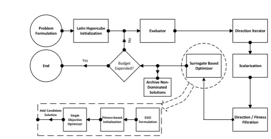
In the current work, ParEGO is treated as a framework rather than a specific algorithm. The implementation of ParEGO differs slightly from the original in ways outlined below. The implementation has been undertaken inTigon, which is

an open-source C++ library that has been developed to support theLiger

open-source optimization workflow software [6]. In Tigon, an optimization algorithm is assembled from a set of components according to the Decorator design pattern. Figure 1 depicts a workflow diagram for the new implementation of ParEGO.

This implementation of ParEGO begins by defining an optimization prob-lem. Next, an initial population is created using LHS and is evaluated on the high-fidelity evaluation functions. Next, the Direction Iterator creates a set of weight vectors according to generalised decomposition [5] and randomly chooses from amongst them. Subsequently, the Scalarization operator applies the weights to the Lp-norm scalarization function (P

k

i=1ωi|fi(x)−zi∗|

p₎1_{p, where}

wi is the

weight of the ith objective, fi(x) is the evaluation of a solution x on the ith

objective, z⋆

i relates to the ideal point, and p is the order of the scalarisation

Latin Hypercube

Initialization Evaluator Direction Iterator

Scalarization Problem

Formulation

Direction / Fitness Filtration Surrogate Based

Optimizer

Budget Expended?

N

o

End

Yes

EGO Formulation Fitness-based

Initialization Single

Objective Optimizer

Archive Non Dominated Solutions

Add Candidate Solution

Fig. 1.Implemented framework for ParEGO

DACE model is constructed and searched over using the efficient single-objective optimizer ACROMUSE [12], which is the default evolutionary optimizer imple-mented in Tigon. A new solution is identified, evaluated, and the optimizer iter-ates until the evaluation budget is expended. All solutions are archived off-line as the search progresses, with the archive filtered for non-dominated solutions.

3

Experiments with scalarising norms

We employ a formal hypothesis testing framework to explore the effect of differ-ent scalarising norm choices on the performance of ParEGO.

3.1 Hypotheses

1. To obtain good coverage of the Pareto front, the scalarising norm must be of a higher-order than the shape of the front (see [13] for the geometric analysis relating scalarisation functions to Pareto dominance relations).

2. In the case where two different scalarising norms are of sufficient order to capture the front, the lower-order norm will converge faster than the higher-order norm (see [5] for underpinning argumentation and experiments). 3. By increasing the order of the norm dynamically during an optimization

run, enhanced convergence can be achieved for problems where higher-order norms are needed to capture the shape of the front.

3.2 Test problems and performance indicators

generational distance (IGD) [17]. The hypervolume reference point is defined as the anti-ideal. Raw hypervolume values are normalised with respect to the hypervolume of the global Pareto front. Metrics are applied to the off-line archive.

3.3 Experimental set-up

To implement the hypothesis tests, we consider a set of experiments that are repeated for optimizers using a range of static and dynamic scalarising norms.

Static norm experiments:These tests try to validate or reject hypotheses

1 and 2. The experiment has 6 categories of tests (outlined in Table 1) and in each of those tests three norms ofp∈ {1,2,∞}are tested with the same initial population on convex and concave versions of DTLZ2. The budget for evalua-tion for these tests, including the initial populaevalua-tion defined using LHS, is the following: 1400 evaluations for two-objective tests (CAT1-2), 1800 evaluations for four-objective tests (CAT3-4) and 2000 evaluations for seven-objective tests (CAT5-6). These budgets are larger than allowable for some industrial problems but enable long-run convergence to be observed. The expected outcome for the convex problem is that all norms can capture the Pareto front given a sufficiently high budget, with the lower-order norms achieving this result more quickly with

norm p= 1 expected to be fastest. As for the concave tests, normp=∞ will

capture the Pareto front, norm p= 2 will partly capture the Pareto front and

normp= 1 will only capture the extremes of the front.

Dynamic norm experiments:These tests implement ParEGO with a

pre-defined schedule of changing norms in order to confirm or reject hypothesis 3. Again six test categories were created with the parameters following the same setup as in Table 1; however budget size and implementation of norms in these experiments is different. For a given budget of 500 evaluations, which excludes the initial population size, the budget is divided into four quarters: the first quarter begins with thep= 1 norm, at the beginning of the second quarter the

norm is switched to p= 2, at the beginning of the third quarter norm p= 50

comes into effect, and at the beginning of the fourth quarter the Tchebycheff norm (p=∞) is operating. The expected outcome for concave geometries is for the norm scheduled version to outperform all static cases. For convex geometries,

performance is expected to be better than staticp=∞but worse thanp= 1.

Both types of experiment are repeated for k ∈ {2,4,7}. In all tests, the number of decision variables that comprise the distance function ‘g’ in DTLZ2 and DTLZ2CX is fixed at 5, so that the total number of decision variables is

d = k+ 4. The number of weight vectors is determined by s = 3. The initial

population size for LHS follows the original guidelines set by Knowles of 11d−1 and the maximum number of solutions chosen to estimate the DACE model is 80 (again, following Knowles). All experiments were replicated 11 times.

4

Results — static norms

trajecto-Table 1.Experimental configuration for 6 categories of test

Test category

Decision vector size

Objective vector size

Number of directions

Initial population

size

DACE surrogate

size

Pareto front geometry

CAT1 6 2 10 65 80 Concave

CAT2 6 2 10 65 80 Convex

CAT3 8 4 20 87 80 Concave

CAT4 8 4 20 87 80 Convex

CAT5 11 7 84 120 80 Concave

CAT6 11 7 84 120 80 Convex

ries shown fori= [1, 500] andi= [501, 1000] to indicate trends on alternative budgets. Box plots for IGD metrics summarising performance across the 11 runs are shown fori= 500 andi= 1000. Scatterplots and parallel coordinates plots are also included as needed to support understanding of the results.

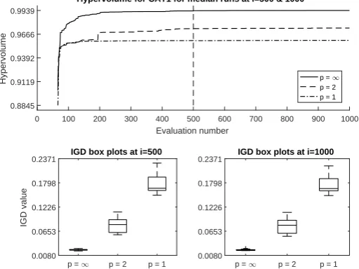
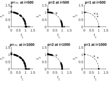
2-objective instances: Results for the concave CAT1 test are shown in

Figure 2. p= ∞ outperforms p = 1 and p = 2 in terms of both median HV

and the IGD distribution. Scatterplots of median HV runs (Figure 3) show that

p = 1 has found good quality solutions only at the edges of the global front

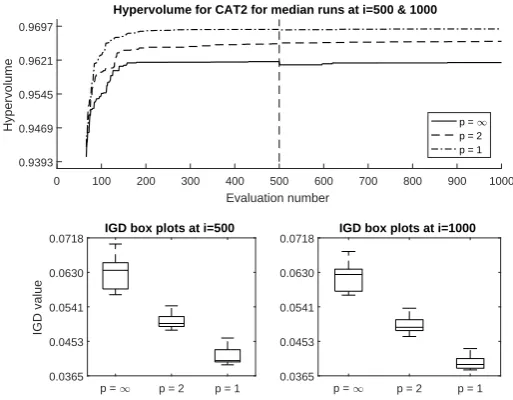
(the latter is indicated by the dashed line in the plots). For the convex CAT2

tests,p= 1 andp= 2 show more rapid convergence thanp=∞for the median

run, although the IGD results are inconclusive (see Figure 4) . Scatterplots for median runs (not shown) all indicate good convergence to the global front.

0 100 200 300 400 500 600 700 800 900 1000

Evaluation number 0.8845

0.9119 0.9392 0.9666 0.9939

Hypervolume

Hypervolume for CAT1 for median runs at i=500 & 1000

p = 1

p = 2 p = 1

p = 1 p = 2 p = 1 0.0080

0.0653 0.1226 0.1798 0.2371

IGD value

IGD box plots at i=500

p = 1 p = 2 p = 1 0.0080

0.0653 0.1226 0.1798

0.2371 IGD box plots at i=1000

0 0.5 1 1.5 f₁ 0 0.5 1 1.5 f2

p=1 at i=500

0 0.5 1 1.5 f₁ 0 0.5 1 1.5 f2

p=2 at i=500

0 0.5 1 1.5 f₁ 0 0.5 1 1.5 f2

p=1 at i=500

0 0.5 1 1.5 f₁ 0 0.5 1 1.5 f2

p=1 at i=1000

0 0.5 1 1.5 f₁ 0 0.5 1 1.5 f2

p=2 at i=1000

0 0.5 1 1.5 f₁ 0 0.5 1 1.5 f2

p=1 at i=1000

Fig. 3.Scatterplots relating to median HV runs for static CAT1 tests

4-objective instances: As shown in Figure 5, for the 4-objective concave

CAT3 test, p= ∞ does not exhibit the clear outperformance seen previously

for k= 2. This appears to be as a result of slower convergence, but this result

is curiously not replicated on the convex CAT4 (see Figure 6), where p = ∞

exhibits similar convergence top= 1 andp= 2.

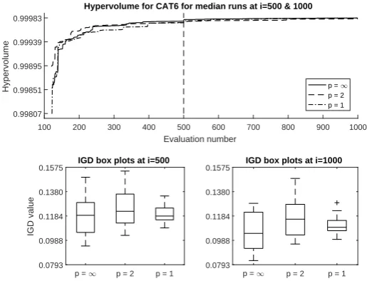
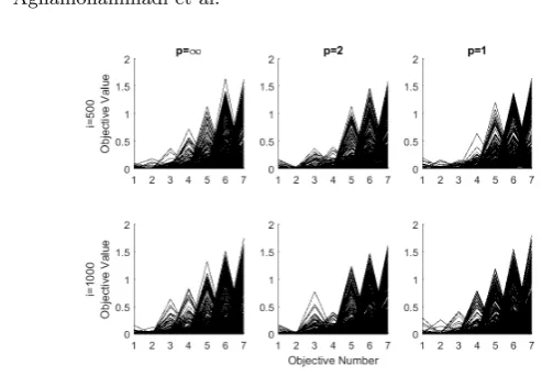
7-objective instances:The situation for the 7-objective concave CAT5 test

is similar to the finding for k= 4 and is not shown. For the convex CAT6 case (shown in Figure 7), the median run forp= 1 suffers slow convergence but the IGD results indicate substantial inter-run variability. Parallel coordinates plots corresponding to the median HV results (see Figure 8) suggest that all norms are struggling to converge to the global front.

The 2-objective results offer support for hypotheses 1 and 2 – withp=∞

offering better coverage of concave fronts, but with a convergence speed penalty compared top= 1 andp= 2 for convex fronts. The 4-objective and 7-objective results, by contrast, offer less support to these hypotheses, with all norms suf-fering convergence issues within the available limited budget.

5

Results – dynamic norms

Many different possibilities exist for applying dynamic norms within ParEGO. Here, for simplicity, after initialisation the remaining budget is divided into quar-ters and the norm is increased over the course of the optimization process.p= 1, p= 2,p= 50, andp=∞are used in each successive quarter. Experiments are run for a total budget of 500 evaluations (exclusive of the budget used for ini-tialisation). The categories of tests remain the same as in the static experiments.

Convergence profiles relate to the run with the median HV ati= 500.

Compar-isons are made to the equivalent results for thep= 1 and p=∞norms.

2-objective instances: The results for the dynamic CAT1 test on the

0 100 200 300 400 500 600 700 800 900 1000 Evaluation number

0.9393 0.9469 0.9545 0.9621 0.9697

Hypervolume

Hypervolume for CAT2 for median runs at i=500 & 1000

p = 1

p = 2 p = 1

p = 1 p = 2 p = 1 0.0365

0.0453 0.0541 0.0630 0.0718

IGD value

IGD box plots at i=500

p = 1 p = 2 p = 1 0.0365

0.0453 0.0541 0.0630

0.0718 IGD box plots at i=1000

Fig. 4.HV convergence profiles and IGD box plots for static CAT2 tests

0 100 200 300 400 500 600 700 800 900 1000

Evaluation number 0.8708

0.8985 0.9262 0.9539 0.9817

Hypervolume

Hypervolume for CAT3 for median runs at i=500 & 1000

p = 1

p = 2 p = 1

p = 1 p = 2 p = 1 0.2262

0.2415 0.2568 0.2720 0.2873

IGD value

IGD box plots at i=500

p = 1 p = 2 p = 1 0.2262

0.2415 0.2568 0.2720

0.2873 IGD box plots at i=1000

0 100 200 300 400 500 600 700 800 900 1000 Evaluation number

0.98646 0.98724 0.98801 0.98879 0.98957

Hypervolume

Hypervolume for CAT4 for median runs at i=500 & 1000

p = 1 p = 2 p = 1

p = 1 p = 2 p = 1 0.0671

0.0715 0.0759 0.0803 0.0848

IGD value

IGD box plots at i=500

p = 1 p = 2 p = 1 0.0671

0.0715 0.0759 0.0803

0.0848 IGD box plots at i=1000

Fig. 6.HV convergence profiles and IGD box plots for static CAT4 tests

100 200 300 400 500 600 700 800 900 1000

Evaluation number 0.99807

0.99851 0.99895 0.99939 0.99983

Hypervolume

Hypervolume for CAT6 for median runs at i=500 & 1000

p = 1 p = 2 p = 1

p = 1 p = 2 p = 1 0.0793

0.0988 0.1184 0.1380 0.1575

IGD value

IGD box plots at i=500

p = 1 p = 2 p = 1 0.0793

0.0988 0.1184 0.1380

0.1575 IGD box plots at i=1000

Fig. 8.Parallel coordinates plots relating to median HV runs for static CAT6 tests

scheme to improve convergence over thep= 1 static scheme is clear, with

tran-sitions to HV values superior to the saturated p = 1 results as the order of

the norm is increased. The final result at the end of the optimization budget

is close to the p = ∞ performance. No convergence acceleration advantage is

seen during the early stages of the search, reflecting the result already seen for the static CAT1 tests. For the bi-objective convex problem (see Figure 10), the median HV results suggest some deterioration in convergence speed arising from the progression to higher-order norms in the latter stages of the optimization process; this finding is confirmed by the IGD results, suggesting that there is a penalty in terms of convergence when the higher-order norm is unnecessary.

4-objective instances:The results for the 4-objective concave problem are

shown in Figure 11. The median HV result indicates that the dynamic scheme has offered a speed-up over the static p= ∞ alternative, whilst retaining the benefits of improved coverage of the front; however the IGD results suggest that

the performance benefits over p= ∞ are inconclusive when considering all 11

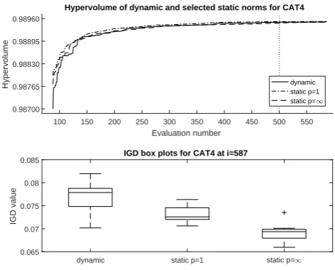
runs. In the static CAT4 tests (shown in Figure 12), whilst it is unsurprising

that the dynamic scheme is unable to outperform the p = 1 equivalent, the

deterioration in search speed shown for the median HV in the early stages of the search is unexpected. This sits alongside the previous unexpected strong performance ofp=∞reported earlier.

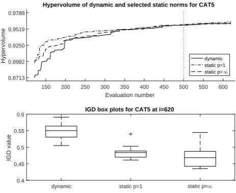
7-objective instances:The parallel coordinates plots in Figure 8 have

al-ready indicated the problems encountered by the static schemes in converging to the global front of the 7-objective CAT5 and CAT6 tests. In the concave CAT5 test, the median HV result shows surprisingly poor performance in the early

part of the search in comparison to both the p= 1 andp=∞cases; however

performance is similar across all three schemes by the end of the budget. Looking across all 11 runs, the IGD results hint – again, surprisingly – that the dynamic

scheme might be faring worse thanp= 1 on this concave problem. Results for

50 100 150 200 250 300 350 400 450 500 550 Evaluation number

0.8845 0.9120 0.9395 0.9669 0.9944

Hypervolume

Hypervolume of dynamic and selected static norms for CAT1

dynamic static p=1 static p=1

dynamic static p=1 static p=1

0 0.05 0.1 0.15 0.2 0.25

IGD value

IGD box plots for CAT1 at i=565

Fig. 9.HV convergence profiles and IGD box plots for dynamic CAT1 tests

50 100 150 200 250 300 350 400 450 500 550 Evaluation number

0.9403 0.9477 0.9550 0.9623 0.9696

Hypervolume

Hypervolume of dynamic and selected static norms for CAT2

dynamic static p=1 static p=1

dynamic static p=1 static p=1

0.03 0.04 0.05 0.06 0.07

IGD value

IGD box plots for CAT2 at i=565

100 150 200 250 300 350 400 450 500 550 Evaluation number

0.8498 0.8831 0.9164 0.9497 0.9830

Hypervolume

Hypervolume of dynamic and selected static norms for CAT3

dynamic static p=1 static p=1

dynamic static p=1 static p=1

0.22 0.24 0.26 0.28 0.3

IGD value

IGD box plots for CAT3 at i=587

Fig. 11.HV convergence profiles and IGD box plots for dynamic CAT3 tests

100 150 200 250 300 350 400 450 500 550 Evaluation number

0.98700 0.98765 0.98830 0.98895 0.98960

Hypervolume

Hypervolume of dynamic and selected static norms for CAT4

dynamic static p=1 static p=1

dynamic static p=1 static p=1

0.065 0.07 0.075 0.08 0.085

IGD value

IGD box plots for CAT4 at i=587

150 200 250 300 350 400 450 500 550 600 Evaluation number

0.8713 0.8982 0.9250 0.9519 0.9788

Hypervolume

Hypervolume of dynamic and selected static norms for CAT5

dynamic static p=1 static p=1

dynamic static p=1 static p=1

0.4 0.45 0.5 0.55 0.6

IGD value

IGD box plots for CAT5 at i=620

Fig. 13.HV convergence profiles and IGD box plots for dynamic CAT5 tests

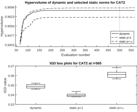
The bi-objective experiments offer partial support to hypothesis 3. For the concave geometry, the dynamic scheme showed little deterioration over using a staticp=∞, but no speed-up was observed during the early stages of the search. It is possible that this finding may be because DTLZ2 with only 5 variables in the ‘g’ function is an easy problem to solve. Meanwhile, the dynamic result on the convex problem supported hypothesis 3, offering improved performance over p=∞. The 4-objective experiment on the concave problem is similar to the bi-objective result (offering partial support to hypothesis 3), but the result in the convex case is confounded by the curious, rapid convergence of the staticp=∞ norm. The 7-objective experiments offer no support to hypothesis 3, with some evidence that the dynamic approach is actually harmful to convergence.

6

Conclusion

for dynamic adjustment of the norm (from lower-order earlier in the search to higher-order later in the search) to overcome the trade-off implied by hypotheses 1 and 2 for problems with concave geometries. Our experiments showed that, for bi-objective concave problems, the dynamic norm was a more favourable choice thanp= 1 but did not offer accelerated convergence overp=∞and, as such, did not represent a ‘dominating’ option. This favourability was retained in the 4-objective case, but had disappeared in the 7-objective case. Overall, the findings suggest that ParEGO (at least in the new implementation) may not be performing well for many-objective problems.

6.1 Limitations and future work

This project was limited by the resource constraints imposed on a 3-month post-graduate project. In a number of cases, convergence trajectories were slow but had not completely saturated within the number of evaluations available and it would have been useful to further understand these convergence trends. The number of replications was limited to 11, which is less than is desirable for robust statistical analysis. Specifically here, it would be interesting to further examine the apparent deterioration of the dynamic scheme in the 7-objective cases. We were also limited in the number of test problems for which we could investigate performance – DTLZ2 and its convex hybrid captured the Pareto front geome-tries of interest to our hypotheses, but it would have been potentially insightful to explore other (particularly, more challenging) problem formulations. In par-ticular, it would be interesting to consider mixed convex-concave surfaces and asymmetrical problems. The dynamic norm scheme we implemented was quite crude and should be seen as a basis for further exploration. Such further work could involve both sensitivity analysis for schemes with a priori norm scheduling, but also consider adaptive schemes based around on-line convergence metrics.

Acknowledgments. This work was supported by Jaguar Land Rover and the

UK-EPSRC grant EP/L025760/1 as part of the jointly funded Programme for

Simula-tion InnovaSimula-tion. The authors thank Joshua Knowles for discussions on ParEGO and surrogate-based optimization that helped inspire the research directions in this paper.

This manuscript is the open-access version of: Aghamohammadi N.R. et al.On the

Effect of Scalarising Norm Choice in a ParEGO Implementation. In: H. Trautmann et al. (Eds.): EMO 2017, LNCS 10173, pp. 1-15, 2017. The final publication is available

at Springer viahttp://dx.doi.org/10.1007/978-3-319-54157-0_1.

References

1. Cristescu, C., Knowles, J.: Surrogate-based multiobjective optimization: ParEGO update and test. In: Workshop on Computational Intelligence (UKCI) (2015) 2. Davins-Valldaura, J., Moussaoui, S., Pita-Gil, G., Plestan, F.: ParEGO

3. Deb, K., Thiele, L., Laumanns, M., Zitzler, E.: Scalable test problems for evolu-tionary multiobjective optimization. Springer (2005)

4. Fonseca, C.M., Paquete, L., L´opez-Ib´anez, M.: An improved dimension-sweep

al-gorithm for the hypervolume indicator. In: 2006 IEEE International Conference on Evolutionary Computation. pp. 1157–1163. IEEE (2006)

5. Giagkiozis, I., Fleming, P.J.: Methods for multi-objective optimization: An analy-sis. Information Sciences 293, 338–350 (2015)

6. Giagkiozis, I., Lygoe, R.J., Fleming, P.J.: Liger: an open source integrated opti-mization environment. In: Proceedings of the 15th Annual Conference Companion on Genetic and Evolutionary Computation. pp. 1089–1096. ACM (2013)

7. Horn, D., Wagner, T., Biermann, D., Weihs, C., Bischl, B.: Model-based multi-objective optimization: taxonomy, multi-point proposal, toolbox and benchmark. In: International Conference on Evolutionary Multi-Criterion Optimization. pp. 64–78. Springer (2015)

8. Huband, S., Hingston, P., Barone, L., While, L.: A review of multiobjective test problems and a scalable test problem toolkit. IEEE Transactions on Evolutionary Computation 10(5), 477–506 (2006)

9. Jeong, S., Obayashi, S.: Efficient global optimization (EGO) for multi-objective problem and data mining. In: 2005 IEEE Congress on Evolutionary Computation. vol. 3, pp. 2138–2145. IEEE (2005)

10. Jones, D.R., Schonlau, M., Welch, W.J.: Efficient global optimization of expensive black-box functions. Journal of Global optimization 13(4), 455–492 (1998) 11. Knowles, J.: ParEGO: a hybrid algorithm with on-line landscape approximation

for expensive multiobjective optimization problems. IEEE Transactions on Evolu-tionary Computation 10(1), 50–66 (2006)

12. Mc Ginley, B., Maher, J., O’Riordan, C., Morgan, F.: Maintaining healthy popula-tion diversity using adaptive crossover, mutapopula-tion, and selecpopula-tion. IEEE Transacpopula-tions on Evolutionary Computation 15(5), 692–714 (2011)

13. Miettinen, K., Ruiz, F., Wierzbicki, A.P.: Introduction to multiobjective optimiza-tion: interactive approaches. In: Multiobjective Optimization, pp. 27–57. Springer (2008)

14. Ponweiser, W., Wagner, T., Biermann, D., Vincze, M.: Multiobjective optimiza-tion on a limited budget of evaluaoptimiza-tions using model-assisted s-metric selecoptimiza-tion. In: International Conference on Parallel Problem Solving from Nature. pp. 784–794. Springer (2008)

15. Scheff´e, H.: Experiments with mixtures. Journal of the Royal Statistical Society. Series B (Methodological) pp. 344–360 (1958)

16. Tabatabaei, M., Hakanen, J., Hartikainen, M., Miettinen, K., Sindhya, K.: A sur-vey on handling computationally expensive multiobjective optimization problems using surrogates: non-nature inspired methods. Structural and Multidisciplinary Optimization 52(1), 1–25 (2015)

17. Van Veldhuizen, D.A., Lamont, G.B.: On measuring multiobjective evolutionary algorithm performance. In: Evolutionary Computation, 2000. Proceedings of the 2000 Congress on. vol. 1, pp. 204–211. IEEE (2000)

18. Voutchkov, I., Keane, A.: Multi-objective optimization using surrogates. In: Com-putational Intelligence in Optimization, pp. 155–175. Springer (2010)

19. Wagner, T.: Planning and Multi-objective Optimization of Manufacturing Pro-cesses by Means of Empirical Surrogate Models. Ph.D. thesis (2013)

budgets. In: International Conference on Evolutionary Multi-Criterion Optimiza-tion. pp. 756–770. Springer (2013)