This is a repository copy of
A methodology for efficient code optimizations and memory
management
.
White Rose Research Online URL for this paper:
http://eprints.whiterose.ac.uk/130673/
Version: Accepted Version
Proceedings Paper:
Kelefouras, V and Djemame, K orcid.org/0000-0001-5811-5263 (2018) A methodology for
efficient code optimizations and memory management. In: CF '18 Proceedings of the 15th
ACM International Conference on Computing Frontiers. ACM International Conference on
Computing Frontiers 2018, 08-10 May 2018, Ischia, Italy. ACM , pp. 105-112. ISBN
978-1-4503-5761-6
https://doi.org/10.1145/3203217.3203274
(c) 2018, ACM. This is the author's version of the work. It is posted here for your personal
use. Not for redistribution. The definitive Version of Record was published in 'CF '18
Proceedings of the 15th ACM International Conference on Computing Frontiers',
https://doi.org/10.1145/3203217.3203274
[email protected]
https://eprints.whiterose.ac.uk/
Reuse
Items deposited in White Rose Research Online are protected by copyright, with all rights reserved unless
indicated otherwise. They may be downloaded and/or printed for private study, or other acts as permitted by
national copyright laws. The publisher or other rights holders may allow further reproduction and re-use of
the full text version. This is indicated by the licence information on the White Rose Research Online record
for the item.
Takedown
If you consider content in White Rose Research Online to be in breach of UK law, please notify us by
management
Vasilios Kelefouras
University of Leeds [email protected]Karim Djemame
University of Leeds [email protected]ABSTRACT
The key to optimizing software is the correct choice, order as well parameters of optimizations-transformations, which has remained an open problem in compilation research for decades for various rea-sons. First, most of the compilation subproblems-transformations are interdependent and thus addressing them separately is not effec-tive. Second, it is very hard to couple the transformation parameters to the processor architecture (e.g., cache size and associativity) and algorithm characteristics (e.g. data reuse); therefore compiler de-signers and researchers either do not take them into account at all or do it partly. Third, the search space (all different transformation parameters) is very large and thus searching is impractical.
In this paper, the above problems are addressed for data dom-inant affine loop kernels, delivering significant contributions. A novel methodology is presented that takes as input the underlying architecture details and algorithm characteristics and outputs the near-optimum parameters of six code optimizations in terms of either L1,L2,DDR accesses, execution time or energy consumption. The proposed methodology has been evaluated to both embedded and general purpose processors and for 6 well known algorithms, achieving high speedup as well energy consumption gain values over gcc compiler, hand written optimized code and Polly.
KEYWORDS
Code optimizations, data cache, register blocking, loop tiling, high performance, energy consumption, data reuse
ACM Reference format:
Vasilios Kelefouras and Karim Djemame. 2016. A methodology for effi-cient code optimizations and memory management. InProceedings of ACM Conference, Washington, DC, USA, July 2017 (Conference’17),8 pages. DOI: 10.1145/nnnnnnn.nnnnnnn
1
INTRODUCTION
Although significant advances have been made in developing ad-vanced compiler optimization and code transformation frameworks, current compilers cannot compete hand optimized code in terms of performance and energy consumption. Researchers tackle the code optimization problem by using heuristics [12], empirical tech-niques, iterative compilation techniques [11] and techniques that simultaneously optimize only two transformations, e.g., register al-location and instruction scheduling. The most promising approach
Permission to make digital or hard copies of all or part of this work for personal or classroom use is granted without fee provided that copies are not made or distributed for profit or commercial advantage and that copies bear this notice and the full citation on the first page. Copyrights for components of this work owned by others than ACM must be honored. Abstracting with credit is permitted. To copy otherwise, or republish, to post on servers or to redistribute to lists, requires prior specific permission and/or a fee. Request permissions from [email protected].
Conference’17, Washington, DC, USA
© 2016 ACM. 978-x-xxxx-xxxx-x/YY/MM. . . $15.00 DOI: 10.1145/nnnnnnn.nnnnnnn
is iterative compilation but is extremely expensive in terms of com-pilation time; therefore researchers and current compilers try to reduce compilation time by using i) both iterative compilation and machine learning compilation techniques [20], ii) both iterative compilation and genetic algorithms [11], iii) heuristics and em-pirical methods [5], iv) both iterative compilation and statistical techniques, v) exhaustive search [10]. However, by employing these approaches, the remaining search space is still so large that searching is impractical. The end result is that seeking the optimal configuration is impractical even by using modern supercomputers. This is evidenced by the fact that most of the iterative compilation methods use either low compilation time transformations only or high compilation time transformations with partial applicability so as to keep the compilation time in a reasonable level [9] [19] [13]. As a consequence, a very large number of solutions is not tested. This has led compiler researchers to use exploration prediction mod-els focusing on beneficial areas of optimization search space [5]. Our approach differs in three main aspects. First, the transforma-tions are addressed in a theoretical basis; second, together as one problem, and third by taking into account the Hardware (HW) ar-chitecture and algorithm characteristics. This way, the search space is reduced by orders of magnitude and as a consequence the quality of the end result is significantly improved.
The main steps of our methodology are as follows. First, we pro-vide an efficient register blocking and loop tiling algorithm; these two algorithms consist of a) loop unroll, scalar replacement, register allocation and b) loop tiling, data array layout, transformations, respectively. A unified framework is proposed to orchestrate the aforementioned transformations, together as one problem (as they are interdependent); the transformations are tailored to the target processor architecture details and algorithm characteristics. Sec-ond, we make an analysis of how the above transformations affect Execution Time (ET) and Energy consumption (E) and for the first time we provide a theoretical model describing a) the number of L1 data cache (L1dc), L2 cache (L2c) and main memory (MM) accesses and b) the number of arithmetical instructions, as a function of the aforementioned transformation parameters, processor architecture details and algorithm input size; so, we are able to provide the trans-formation parameters giving a number of memory accesses close to the minimum. Third, taking advantage of this model, we make a first but important step towards correlating ET and E with the aforementioned transformation parameters, processor architecture details and algorithm input size.
Conference’17, July 2017, Washington, DC, USA V. Kelefouras et al.
patterns, 3) a theoretical model describing the number of mem-ory accesses and arithmetical instructions, as a function of the aforementioned optimization parameters, HW architecture and al-gorithm input size, 4) a new approach correlating ET and Power consumption (P) with the aforementioned transformation parame-ters, HW architecture and algorithm input size, 5) a direct outcome of contributions (1)-(4) is that the search space (to fine-tune the above optimizations) is reduced by many orders of magnitude.
Our obtained evaluation results which have been carried out using two real processors, gem5 [3] and mcpat [14] simulators, are reported in terms of L1/L2/DDR memory accesses, arithmetical instructions, ET, P and E.
The remainder of this paper is organized as follows. In Section 2, the related work is reviewed. The proposed methodology is pre-sented in Section 3 while experimental results are discussed in Section 4. Finally, Section 5 is dedicated to conclusions.
2
RELATED WORK
Iterative compilation methods provide the most efficient approach towards the code optimization problem. However, to the best of our knowledge, there is no existing iterative compilation method including all the transformations presented in this paper and all different transformation parameters, because the compilation time becomes too large. Iterative compilation methods use either low compilation time transformations only or high compilation time transformations with partial applicability so as to keep the com-pilation time in a reasonable level [9] [19]. As a consequence, a very large number of solutions is not tested. In [19], loop tiling is applied with fixed tile sizes. In [9], multiple levels of tiling are applied but with fixed tile sizes. In [13], only loop unroll is applied. [12] uses an artificial neural network to predict the best trans-formation (from a given set) should applied. In [5], performance counters are used to determine good compiler optimization settings. In [20], a long-term learning algorithm that determines the best set of heuristics is presented.
The polyhedral model is a flexible and expressive representation for loop transformations. In [17], a fundamental progress in the understanding of polyhedral loop nest optimizations is made. Polly is a high-level loop and data-locality optimizer and optimization infrastructure for LLVM [6]. Pluto, which is used by Polly, is an automatic parallelization tool based on the polyhedral model [4].
There has been significant research on reducing the number of data accesses in memory hierarchy by employing compiler trans-formations and most commonly loop tiling such as [4] [15]. In [15], a cache hierarchy aware tile scheduling algorithm for multicore architectures is presented.
Code optimizations are also used to reduce energy consumption in software. In [1], a survey about energy reduction methods is given. In [16], several transformation trade-offs are discussed. In [2], a compile-time approach to determine CPU frequency is proposed.
3
PROPOSED METHODOLOGY
In this paper, a novel methodology is presented that takes as input the underlying processor architecture and loop kernel character-istics and outputs the near-optimum parameters of the six afore-mentioned transformations in terms of either L1,L2,DDR accesses, Execution Time (ET) or Energy consumption (E).
Regarding target applications, this methodology considers affine loop kernels; it considers both perfectly and imperfectly nested loops, where all the array subscripts are linear equations of the iterators (which stands in most cases). This method is also applica-ble to loop kernels containing SIMD instructions. This method is applicable to all modern single-core and shared cache multi-core CPUs. Regarding shared cache processors, we use the software shared cache partitioning method given in our previous work [8].
No more thanpthreads can run in parallel (one to each core), where
pis the number of the processing cores (single threaded codes only).
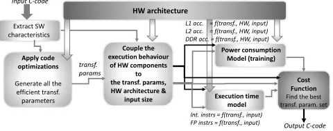
An abstract representation of our method is illustrated in Fig. 1 and it is further explained in the following Subsections.
Input C-code
HW architecture
Apply code optimizations
Generate all the efficient transf. parameters Extract SW characteristics
Couple the execution behaviour
of HW components to the transf. params, HW architecture &
input size Execution time model Power consumption
Model (training)
Cost Function Find the best transf. param. set
transf. params
L1 acc. = f(transf., HW, input) L2 acc. = f(transf., HW, input) DDR acc. = f(transf., HW, input)
Int. instrs = f(transf., input)
[image:3.612.321.561.233.328.2]FP instrs = f(transf., input) Output C-code
Figure 1: Flow chart of the proposed methodology
3.1
Apply code optimizations
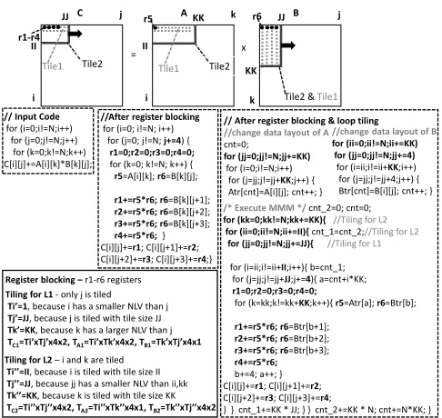
In this Subsection we provide an efficient a) register blocking and b) loop tiling algorithm. The efficient application of loop tiling is not trivial and normally many different implementations are tested, since it a) depends on other transformations (e.g., data layout), b) depends on the target memory architecture and data reuse, c) in-creases the number of arithmetical instructions. The application of loop tiling for the Register File (RF) is even more complex (register blocking). To our knowledge, no application independent algo-rithm exists for register blocking; it is a mixture of loop tiling, loop unroll, scalar replacement and register allocation transformations. The above CO are the key to high performance and low energy consumption, especially for data dominant algorithms.
The main steps of the proposed register blocking algorithm are the following:
(1) Generate the subscript equations of all arrays
(2) Generate the RF inequality (Eq. 1) that provides all the efficient transformation parameters
(3) Extract a transformation set from Eq. 1 (4) Generate the code
Definition 3.1. Subscript equations which have more than one
solution for at least one constant value, are named type2 equations. All others, are named type1 equations.
For example, (A[2∗i+j]) gives the following type2 equation
(2∗i+j =c1), while (A[i][j]) gives the following type1 equation (i=c21 andj=c22).
The RF inequality (Eq. 1) gives the exact loops that loop unroll is applied to, their unroll factor values and the number of vari-ables/registers allocated for each array. Each subscript equation
contributes to the creation of Eq. 1, i.e., equationigivesAriand
specifies its expression. The implementations that do not obey to the extracted inequalities are discarded reducing substantially the search space. The RF inequality is given by
n+Sc≤Ar1+Ar2+. . .+Arn+Sc≤F P (1)
whereF Pis the number of the floating point (FP) registers,Sc
is the number of FP scalar variables andnis the number of the
array references. Without any loss of generality, we assume that the arrays contain FP data only; in this case, the number of integer variables used is always smaller than the number of integer registers. The upper bound of Eq. 1 derives from the fact that if more registers than the available are used, data are spilled to L1dc, increasing the number of L1 accesses. On the other hand, the lower bound value is small because other constraints may be more critical. By using a larger lower bound value, register utilization is increased and therefore the number of L1 accesses is reduced; however, these transformation parameters may conflict to those minimizing the number of MM or L2 accesses, which may be more critical.
The number of variables/registers allocated for every array is given by both Eq. 2 and the three bullets below (the bullet points are given in order to assign variables according to data reuse).
Ari =unr 1′×unr 2′×. . .×unr n
′ (2)
where the integerunr i′are the unroll factor values of the
iter-ators exist in the array’s subscript, e.g., theC[i][j]array in Fig. 2 gives(ArC=1×4=4)(r1−r4 variables) as the(i,j)iterator unroll
factor values are(1,4), respectively.
• For the type1 arrays which contain all the loop kernel
iterators, only one register is needed (Ari =1)
• For the innermost iterator always holdsunr′=1
• For the arrays i) containing more than one iterators and
one of them is the innermost and ii) all iterators which do not exist in this array reference have unroll factor values equal to 1, then only one register is needed for this array (Ari =1)
In the above three cases, a different element is accessed in each iteration (no data reuse being achieved) and thus wasting more than one register is not efficient, e.g., in Fig. 2, six registers are used,
i.e., (ArC =1×4,ArA=1×1,ArB=1). Note that (ArB=1) instead
of (ArB=1×4) because of the 3rd bullet above (a different element
ofBis accessed in eachkiteration and therefore it is not efficient
to waste more than one register).
Let us give an example, first box code in Fig. 2. Eq. 1 gives:
3≤unri×unrj+unri+unrj ≤F P,unri,1&unrj ,1
3≤unrj+2≤F P,unri =1
3≤unri+2≤F P,unrj =1 (3)
The 3rd bullet generates 3 branches while the 2nd gives(unrk =
1). The code shown in the second box of Fig. 2 refers to a second
branch solution, i.e., (unri = 1 andunrj = 4) and therefore 6
registers are used.
The main steps of the loop tiling algorithm are similar to those of the register blocking algorithm, but a cache inequality (Eq. 4) is generated for each cache memory; each inequality contains the it-erators that loop tiling is applied to, the tile sizes and the data array
/* Execute MMM */ cnt_2=0; cnt=0;
for (kk=0;kk!=N;kk+=KK){ //Tiling for L2
for (ii=0;ii!=N;ii+=II){ cnt_1=cnt_2;//Tiling for L2
for (jj=0;jj!=N;jj+=JJ){ //Tiling for L1
for (i=ii;i!=ii+II;i++){ b=cnt_1; for (j=jj;j!=jj+JJ;j+=4){ a=cnt+i*KK;
r1=0;r2=0;r3=0;r4=0;
for (k=kk;k!=kk+KK;k++){ r5=Atr[a]; r6=Btr[b];
r1+=r5*r6; r6=Btr[b+1];
r2+=r5*r6; r6=Btr[b+2];
r3+=r5*r6; r6=Btr[b+3];
r4+=r5*r6;
b+=4; a++; } C[i][j]+=r1; C[i][j+1]+=r2; C[i][j+2]+=r3; C[i][j+3]+=r4;
} } cnt_1+=KK * JJ; } } cnt_2+=KK * N; cnt+=N*KK; }
//change data layout of B
for (ii=0;ii!=N;ii+=KK) for (jj=0;jj!=N;jj+=4)
for (i=ii;i!=ii+KK;i++) for (j=jj;j!=jj+4;j++) { Btr[cnt]=B[i][j]; cnt++; }
// After register blocking & loop tiling
//change data layout of A
cnt=0;
for (jj=0;jj!=N;jj+=KK)
for (i=0;i!=N;i++) for (j=jj;j!=jj+KK;j++) { Atr[cnt]=A[i][j]; cnt++; }
Tiling for L2 i and k are tiled
T II, because i is tiled with tile size II
Tj JJ, because jj has a smaller NLV than ii,kk
Tk KK, because k is tiled with tile size KK
TC2T T , TA2T T , TB2T T
Tiling for L1 - only j is tiled
Ti , because i has a smaller NLV than j
Tj JJ, because j is tiled with tile size JJ
Tk KK, because k has a larger NLV than j
TC1T T , TA1T T , TB1T T
Register blocking r1-r6 registers
// Input Code
for (i=0;i!=N;i++) for (j=0;j!=N;j++)
for (k=0;k!=N;k++) C[i][j]+=A[i][k]*B[k][j];
C A B
r1-r4
Tile2 & Tile1 II
II
= x
i i
j k j
k
Tile1 Tile2 Tile1 Tile2
JJ r5 KK r6 JJ
KK
//After register blocking
for (i=0; i!=N; i++) for (j=0; j!=N; j+=4) {
r1=0;r2=0;r3=0;r4=0;
for (k=0; k!=N; k++) {
r5=A[i][k]; r6=B[k][j];
r1+=r5*r6; r6=B[k][j+1];
r2+=r5*r6; r6=B[k][j+2];
r3+=r5*r6; r6=B[k][j+3];
r4+=r5*r6; }
[image:4.612.318.561.78.308.2]C[i][j]+=r1; C[i][j+1]+=r2; C[i][j+2]+=r3; C[i][j+3]+=r4;}
Figure 2: An example, Matrix-Matrix Multiplication (MMM)
layouts. The implementations that do not obey to the extracted in-equalities are automatically discarded by our methodology reducing substantially the search space.
The cache inequality is formulated as:
m≤ ⌈ T il e1
Li/assoc⌉+. . .+⌈
T il en
Li/assoc⌉ ≤assoc (4)
whereLiis the corresponding cache size,associs theLi
associa-tivity value (e.g., for an 8-way associative cache,assoc=8) andm
defines the lower bound of the tile sizes and it equals to the number of arrays in the loop kernel. In the special case where the number of the arrays is larger than the associativity value is not discussed in this paper (normally,(assoc≥8)).T ileigives the tile size of the ith array and is given by Eq. 5:
T il ei=T1′×T2′×Tn′ ×type×s (5)
wheretypeis the size of each array’s element in bytes andTi′
are the tile sizes of the iterators existing in the corresponding array
subscript.sis an integer and (s=1 ors=2);sdefines how many
tiles of each array should be allocated in the cache. For the tiles that do not achieve data reuse (a different tile is accessed in each
iteration), we assign cache space twice the size of their tiles (s=2
in Eq. 5). This way, not one but two consecutive tiles are allocated into the cache in order for the second accessed tile not to displace another array’s tile. (⌈ T il e1
Li/assoc⌉) is an integer representing the
number ofLicache lines with identical cache addresses used for
the tile of array1. Eq. 4 satisfies that the array tiles directed to the same cache subregions do not conflict with each other as the number of cache lines with identical addresses needed for the tiles is not larger than the (assoc) value.
Conference’17, July 2017, Washington, DC, USA V. Kelefouras et al.
some special cases where the arrays do not contain consecutive memory locations but their layouts can remain unchanged in order to avoid the cost of transforming the arrays; in that case, extra cache misses occur and thus a larger error in approximating the
number of memory accesses occurs too (Fig. 4-Subsection 4.1).Ti′
is given by one of the following three:
• Ti′equals to the L1 tile size of i iterator, if tiling for L1 is applied to the i iterator
• Ti′equals to the unroll factor value of i iterator, if tiling for L1 is not applied to the i iterator and i has a smaller Nesting Level Value (NLV) than the iterator being tiled for L1
• Ti′equals to the upper loop bound value of i iterator, if
tiling for L1 is not applied to the i iterator and i has a larger NLV than the iterator being tiled for L1
Assuming an 8-way 32kbyte L1dc and MMM (Fig. 2), Eq. 4 gives
(3≤ ⌈TC1
4096⌉+⌈
TA1
4096⌉+⌈
TB1
4096⌉ ≤8). The(TC1,TA1,TB1)values of
the C-code shown at the right of Fig. 2 are given in the bottom
left box (the NLV ofkiterator is 6 while the NLV ofkkis 1), also,
floating point values are assumed, 4 bytes each.
In the shared cache case,Li in Eq. 4 is the corresponding shared
cache partition size used and each core uses only its assigned shared cache space.
We have implemented an automated C to C tool just for the six studied algorithms, but a general tool can be implemented by using POET [18] tool.
3.2
Couple execution behaviour to CO,
processor architecture & input size
For all the Eq. 1 and Eq. 4 schedules, we compute the number of L1dc, L2c and MM accesses as well as the number of arithmetical instructions. This problem is theoretically formulated by exploiting the memory architecture details and the special memory access patterns. In particular, one mathematical equation is generated for each memory and for each loop kernel providing the correspond-ing value. This equation provides the number of memory accesses while the transformation parameters and input size serving as the independent variables of the equation. Loop tiling and loop unroll transformations as well as the input size, are inserted directly to the aforementioned equations while the data layouts, scalar replace-ment and register allocation transformations as well as the HW architecture, are inserted indirectly (they have been used in order to create Eq.1-Eq.5). This way, we are able to find the solution offering a number of L1dc, L2c or MM accesses close to the minimum.
We are able to approximate the number of memory accesses because no unexpected misses occur in the cache. We assume that the underlying memory architecture consists of separate first level data and instruction caches (modern architectures). In this case, the program code typically fits in L1 instruction cache; thus, it is assumed that the shared cache or unified cache (if any) is dominated by data. For the reminder of this paper, we assume 2 levels of cache, but more/less levels can be used, by slightly changing the following equations.
The equation approximating the number of L1dc accesses follows
L1.acc=
i=ar r aysÕ
i=1 (
jÖ=M
j=1
(upj−l owj)
Tj ×
kÖ=P
k=1
unrk+of f seti)+var (6)
wherearraysis the number of arrays,Mis the number of the
iterators that control the corresponding array andPis the number of
the iterators that loop unroll has been applied to (iterators that exist in the subscript of the corresponding array only), e.g., regarding
theCarray in the code at the right of Fig. 2, the first product of
Eq. 6 refers to all the iterators butk(array reference is outsidek
loop) while the second product refers tojiterator only. (up,low)
give the bound values of the corresponding iterator (normally, they define the algorithm’s input size) and(T,unr)refer to the tile size
and unroll factor value, respectively.
o f f setgives the number of L1dc of the new loop kernel added
in the case the data array layout is transformed. Offset is either
(o f f seti =2×ArraySizei) or (o f f seti =0) depending on whether
the data layout of the array is changed or not; in the case that the layout is changed, the array has to be loaded and then written again to memory, thus it is (o f f seti =2×ArraySizei). (var) gives the number of L1 accesses due to the scalar variables; we never use more registers than available and thus the number of RF spills is negligible (var≈0).
Eq. 6 for the C-code at the right of Fig. 2 gives(4×NK K3 ,
N3
4 ,N
3)L1
accesses for(C,A,B)arrays, respectively, and in overall(L1.acc=
N3
4×K K+N
3
4 +N3+4×N2). Here, the number of L1 accesses strongly
depends on the unroll factor value (N3/4).
The number of L2c accesses is approximated by Eq. 7; at this step, only the new/extra iterators (introduced by loop tiling) must be processed and not the initial iterators exist in the input code.
L2Acc.=
Íi=t ype1
i=1 T ype1L2acc.+
Íi=t ype2
i=1 T ype2L2acc.+code (7)
wheretype1 andtype2 is the number oftype1 andtype2 arrays,
respectively. In this paper, we don’t provide the equations for type2 arrays because of the limited paper size; however, in Section 4, FIR
and Gaussian Blur contain type2 arrays.coderefers to the number
of source code accesses and always (Arrays acc.≫code) as a) the
code size of loop kernels is small and fits in L1 instruction cache, b) we are dealing with data dominant algorithms.
Type1L2acc.=array size×ti+o f f set (8)
wherearray sizeis the size of the array ando f f setgives the
number of L2 accesses of the new loop kernel added in the case
the data array layout is transformed.ti gives how many times the
corresponding array is accessed from L2 memory and is given by
Eq. 9. Regarding theo f f setvalue, when the array size is bigger
or comparable to the cache size, then (o f f seti ≻2×ArraySizei).
This is because the elements are always loaded in blocks (cache lines) and many lines are loaded more than once (especially in the column-wise case). This is why we use a hand optimized code changing the layout in an efficient way, thus always achieving
(o f f seti ≈2×ArraySizei).
ti=Îjj==1N
(upj−l owj)
Tj ×
Îk=M
k=1
(upk−l owk)
Tk (9)
whereNis the number of new/extra iterators that a) do not exist
in the corresponding array and b) exist above of the iterators of the
corresponding array.Mis the number of new/extra iterators that a)
do not exist in the array and b) exist between of the iterators of the array, e.g., regarding (C,A,B) arrays in Fig. 2, the iterators referring
to the first and second product of Eq. 9 are (kk,none), (jj,none),
(none,ii), respectively, giving (tC =
N K K), (tA=
N
many times the array is accessed due to the iterators exist above the upper new iterator of this array and between the new iterators of this array, respectively.
Eq. 7 for the code of Fig. 2 gives(L2.acc=N
3/KK
+N3/J J+
N3/I I+4×N2).
In the case that more than one thread run in parallel under a shared cache, the overall number of cache accesses is extracted by accumulating all the different loop kernel equations.
The number of MM accesses is given by an equation identical to Eq. 7. Moreover, the number of MM accesses because of the type1 arrays is given by an equation identical to Eq. 8 and Eq. 9. However, in Eq. 9, we refer only to the iterators created by applying tiling to the last level cache, e.g., regarding (C,A,B) arrays of MMM (Fig. 2),
the iterators referring to the first and second product of Eq. 9 are (kk,none), (none,none), (none,ii), respectively, giving (tC =
N K K), (tA=1) and (tB= NI I), respectively.
The number of integer and FP instructions is approximated by:
Ar it h.inst r s=
i=i t e r at or sÕ
i=1
(
j=i
Ö
j=1
upj−l owj
Tj
×cj)+of f set (10)
whereiteratorsis the total number of iterators and(up,low,T)
are their corresponding bound values, as in previous equations.cjis
the number of integer or FP assembly instructions measured inside
jloop (assembly instructions occur between the open and close
loop bracket).o f f setis the number of arithmetical instructions of
the extra loop kernels added (if the array layouts change). (Íi=it er at or s
i=1 (
Îj=i
j=1 upj−l owj
Tj ) gives the number of loop
itera-tions in total whilecjgives the number of assembly instructions
in loopj. Note thatjiterator varies from (j =1 - it corresponds
to the outermost iterator) to (j=iterators- it corresponds to the
innermost iterator), e.g., in Fig. 2, Eq. 10 gives ((N/KK) ×c1+
(N2/(KK×I I)) ×c2+(N3/(KK×I I×J J)) ×c3+(N3/(KK×J J)) ×
c4+(N3/(KK×4)) ×c5+(N3/4) ×c6); as it can be observed, the number of arithmetical instructions is strongly affected by a) the number of the loops being tiled (more terms are introduced), b) tile size / unroll factor values of the innermost iterators (here, the unroll
factor value ofj, i.e., 4, affects the number of instructions at the
most). Thus, a larger unroll factor value would be more efficient.
Given that thec values depend on the target compiler, they
cannot be approximated. Thus, we measure thecvalues for one
transformation set and predict thecvalues of the others (where
possible), e.g., in Fig. 2, thecvalues (assembly instructions) almost
remain unchanged by changing the (KK,I I,J J) values (apart from
their maximum and minimum ones because in this case, the number
of the loops changes), but not by changing the (j) unroll factor
value or the number of the loops being tiled, because the loop body changes and thus more/less assembly instructions are inserted.
In this work, we take advantage of the fact that thec values
almost remain unchanged for different tile sizes, suffice the array layouts remain unchanged and the tile sizes do not take their
maxi-mum/minimum values; thecvalues are only slightly affected by
the compiler, even by using aggressive compilers and high
opti-mization levels. Thecvalues for different unroll factor values and
data layouts are significantly changed and cannot be predicted.
3.3
Performance Models
The aforementioned transformations affect P and E in all HW com-ponents and thus a different power model is generated for each
[image:6.612.313.566.83.252.2]1 .0 0 E -0 4 1 .0 0 E -0 3 1 .0 0 E -0 2 1 .0 0 E -0 1 1 .0 0 E + 0 0 1 .0 0 E + 0 1 1 .0 0 E + 0 4 1 .0 0 E + 0 5 1 .0 0 E + 0 6 1 .0 0 E + 0 7 Dy na mic P ow er co nsu mp tio n ( lo g. sca le ) N u m b e r o f L 1 d a ta c a ch e a cc e sse s L1 d a ta c a ch e p o w e r co n su m p ti o n m o d e l (4 0 9 6 ,1 6 ,4 ,4 , 2 ,2 , 1 6 ,1 ) (1 6 3 8 4 ,3 2 ,4 ,4 , 2 ,2 , 3 2 ,1 ) (3 2 7 6 8 ,6 4 ,8 ,4 , 2 ,2 , 6 4 ,1 ) (4 0 9 6 ,6 4 ,4 ,1 , 2 ,2 , 6 4 ,1 ) 1 .0 0 E -0 1 1 .0 0 E + 0 0 1 .0 0 E + 0 1 1 .0 0 E + 0 2 1 .0 0 E + 0 4 1 .0 0 E + 0 5 1 .0 0 E + 0 6 1 .0 0 E + 0 7 Dy na mic P ow er co nsu mp tio n ( lo g. sca le ) N u m b e r o f D D R d a ta c a ch e a cc e sse s D D R p o w e r co n su m p ti o n m o d e l (4 ,2 ,4 ) (4 ,1 ,1 ) (2 ,2 ,2 ) (1 ,1 ,1 ) 1 .0 0 E -0 5 1 .0 0 E -0 4 1 .0 0 E -0 3 1 .0 0 E -0 2 1 .0 0 E -0 1 1 .0 0 E + 0 0 1 .0 0 E + 0 4 1 .0 0 E + 0 5 1 .0 0 E + 0 6 1 .0 0 E + 0 7 Dy na mic P ow er co nsu mp tio n ( lo g. sca le ) N u m b e r o f L /S i n st rs, t o ta l i n st rs a n d AL U a cc e sse s, r e sp e ct iv e ly P o w e r co n su m p ti o n m o d e l LO A D Q S T O RE Q In str . B u ff e r In str . D e co d e r in t A LU s
Figure 3: Power consumption models
0 0 .5 1 1 .5 2 2 .5 3 3 .5 4 Err or (%) -Nu mb er of in te ge r i nst ru cti on s T il e si ze s g cc 4 .8 .5 c o m p il e r -C P U i 7 6 7 0 0 m m m m v m fi
r gem
ve r d io tg e n g au ss ia n B lu r 0 1 0 2 0 3 0 4 0 Err or (%) -Nu mb er of in te ge r i nst ru cti on s T il e si ze s g cc 4 .8 .5 c o m p il e r -C P U i 7 6 7 0 0 -h a n d w ri tt e n A V X m m m m v m fi
r gem
ve r d io tg e n g au ss ia n Bl u r 0 1 2 3 4 5 6 7 8 L1 -R e a d s L1 -W ri te s L2 -R e a d s L2 -W ri te s D D R -R e ad s D D R -W ri te s Err or (%) -Nu mb er of me mo ry a cce sses N o rm al c as e m a x e rr o r N o rm al c as e -av e rag e e rr o r S p e ci al c ase -m ax e rr o r S p e ci al c ase -av e rag e e rr o r
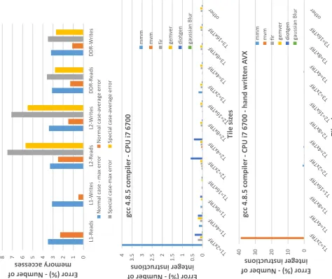
Figure 4: Validation of Eq.6-Eq.10 (relative error)
[image:6.612.319.556.289.488.2]Conference’17, July 2017, Washington, DC, USA V. Kelefouras et al.
P=PL1(f(L1.acc))+PL2(f(L2.acc))+PD D R(f(D DR.acc))+
PL/S Qu eu e(f(L/S.inst r s))+PALU(f(ALU.inst r s))+
Pi ns t r.bu f f e r(f(inst r s))+Pi ns t r.d e c od e r(f(inst r s))
(11)
As far as execution time (ET) is concerned, it cannot be approx-imated by using a mathematical formula; however, we can use current ET models in order to find/predict qualitatively the trans-formation parameter set giving the fastest binary. Given that all the candidate transformation parameter sets a) refer to the same algorithm, b) the algorithm is static, in Subsection 4.1, we show that we are able to select qualitatively a high quality transformation pa-rameter set, even by using a simple execution time model (Average Memory Access Time (AMAT) [7]). Although more accurate and complex ET models exist like [22], where concurrency in memory hierarchy is taken in account, the aim of this first version is to validate and describe the theoretical background.
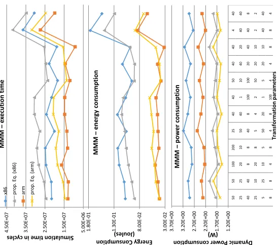
[image:7.612.40.315.271.513.2]5 .0 0 E + 0 6 1 .5 0 E + 0 7 2 .5 0 E + 0 7 3 .5 0 E + 0 7 4 .5 0 E +0 7 Sim ula tio n t im e i n c ycl es MMM e xe cu ti o n t im e x8 6 p ro p . E q . (x 8 6 ) ar m p ro p . E q . (ar m ) 3 .0 0 E -0 2 8 .0 0 E -0 2 1 .3 0 E -0 1 1 .8 0 E -0 1 En erg y C on sum pti on (Jo ule s) MMM e n e rg y c o n su m p ti o n 1 .2 0 E + 0 0 1 .7 0 E + 0 0 2 .2 0 E + 0 0 2 .7 0 E + 0 0 3 .2 0 E + 0 0 3 .7 0 E + 0 0 5 0 5 0 1 0 0 2 0 0 2 5 4 0 4 0 5 0 4 0 4 0 4 4 0 2 5 2 5 2 0 1 0 5 0 4 0 1 1 0 4 0 2 0 4 0 4 0 4 0 4 0 8 8 4 0 8 1 0 0 1 0 0 2 0 4 0 4 0 8 2 5 1 0 2 0 8 5 4 2 5 0 2 0 1 0 2 2 5 2 5 1 0 5 5 0 2 0 1 5 2 0 1 0 4 0 4 0 8 8 4 8 4 8 1 0 0 4 4 8 8 4 Dy na mic P ow er co nsu mp tio n (W ) T ra n sf o rm a ti o n p a ra m e te rs MMM p o w e r co n su m p ti o n
Figure 5: Validation of the ET and P models used (the results for the other algorithms are similar)
3.4
Reduction of the search space - optimality
Although it is impractical to run all different schedules in order to prove that our methodology doesn’t discard efficient schedules, a theoretical explanation is given.
First, the schedules that don’t belong to Eq. 1, either use a larger number of registers than available or they don’t take into account data reuse (and therefore registers are wasted), while the schedules that don’t belong to Eq. 4 either use larger tile sizes than the cache or the tiles cannot remain in the cache. All the above refer to schedules that register blocking and loop tiling have not been applied in an efficient way and therefore they give a high number of data accesses through the whole memory hierarchy. Although Eq. 1 and Eq. 4 transformation parameters do not always provide near-optimum performance as the corresponding transformations are not always
efficient/desirable, Eq. 1 and Eq. 4 do provide all the efficient register blocking and loop tiling implementations, respectively. In other
words, if the target metric is to minimize the number ofLimemory,
then the optimum solution will be included in the corresponding inequality.
3.5
Putting it all together
The proposed methodology is given in Algorithm 1. All the steps have been explained in the previous subsections. All different combinations of loop interchange are generated as it affects Eq.1-Eq.10.
In the case that the target metric is not ET or E, but the minimum
number ofLimemory accesses, then Algorithm 1 is changed
accord-ingly, i.e., steps (1,2,5,8), (1,3,5,8) or (1,4,5,8) are executed only,
respectively. It is important to note that in this case the number of different schedules that have to be further processed by Subsec-tion 3.2 is smaller, i.e., the lower bound values of Eq. 1 and Eq. 4 are no longer needed to be that small. For example, by using a larger lower bound value in Eq. 1, register utilization is increased and therefore the number of L1 accesses is reduced; however, these parameters may conflict to those minimizing the number of MM accesses, which may be more critical. Thus, if the target metric is just the L1dc accesses, there is no need to use such a small Eq. 1 lower bound value. The same holds for L2c and MM too.
Algorithm 1Proposed Methodology
Step 1.parsing
Step 2.apply proposed Register blocking algorithm
for(all different RF sets)do
pick a RF transf. set
Step 3.apply loop tiling alg. to L1
for(all different L1 sets)do
pick an L1 transf. set
Step 4.apply loop tiling alg. to L2
for(all different L2 sets)do
pick an L2 transf. set
Step 5a.generate access equations - Eq. 6-Eq. 9 (all mems)
Step 5b.compute the num of accesses in memory hierarchy
Step 6.arithmetical instructions
if(the num of arith. instrs cannot be predicted for the current set)then
generate C code (from C to C) for the current set generate assembly code - cross compile
measure the num of FP and integer assembly instrs (get the c values of Eq. 10)
else
predict the num of arith. instrs (Eq. 10)
end if
Step 7.compute the ET,P,E values for the current set
Step 8.store only the best set depending on the cost function (ET,E,L1,L2,MM)
end for
apply loop interchange to L2 iterators and go to step4
end for
apply loop interchange to L1 iterators and go to step3
end for
4
EXPERIMENTAL RESULTS
Table 1: Evaluation over gcc and hand written AVX code
MMM - ZYBO MVM - ZYBO
Binaries ET(sec) P (W) E (J) ET(sec) P (W) E (J)
default 1.38E+02 4.80E-01 6.62E+01 4.70E-01 4.10E-01 1.93E-01
best ET 1.55E+01 5.00E-01 7.75E+00 2.20E-01 3.50E-01 7.70E-02
best E 1.79E+01 3.80E-01 6.80E+00 2.20E-01 3.50E-01 7.70E-02
MMM - i7 6700 MVM - i7 6700
default 9.92E+00 4.80E+01 4.76E+02 1.02E-01 4.18E+01 4.25E+00
AVX 8.90E+00 4.66E+01 4.15E+02 8.43E-03 4.67E+01 3.94E-01
best ET 2.30E+00 4.60E+01 1.06E+02 3.30E-03 4.92E+01 1.62E-01
best E 2.40E+00 4.39E+01 1.05E+02 3.30E-03 4.92E+01 1.62E-01
FIR - ZYBO Diotgen - ZYBO
default 1.98E+00 5.75E-01 1.14E+00 3.90E+01 5.00E-01 1.95E+01
best ET 8.20E-01 5.00E-01 4.10E-01 1.60E+00 4.25E-01 6.80E-01
best E 8.60E-01 4.75E-01 4.09E-01 1.60E+00 4.25E-01 6.80E-01
FIR - i7 6700 Diotgen - i7 6700
default 1.33E-01 4.45E+01 5.94E+00 8.90E+00 4.81E+01 4.28E+02
AVX 1.30E-01 4.43E+01 5.76E+00 6.82E+00 4.68E+01 3.19E+02
best ET 3.42E-02 4.70E+01 1.61E+00 2.38E+00 4.55E+01 1.08E+02
best E 3.42E-02 4.70E+01 1.61E+00 2.38E+00 4.55E+01 1.08E+02
Gemver - ZYBO Gaussian Blur - ZYBO
default 4.90E-01 5.75E-01 2.82E-01 2.53E-01 4.10E-01 1.04E-01
best ET 2.10E-01 5.00E-01 1.05E-01 6.65E-02 3.50E-01 2.33E-02
best E 2.10E-01 4.75E-01 9.98E-02 6.65E-02 3.50E-01 2.33E-02
Gemver - i7 6700 Gaussian Blur - i7 6700
default 2.10E-03 4.47E+01 9.39E-02 2.60E-02 4.62E+01 1.20E+00
AVX 2.00E-03 3.70E+01 7.40E-02 6.10E-03 4.68E+01 2.85E-01
best ET 1.54E-03 3.65E+01 5.62E-02 5.40E-03 4.64E+01 2.51E-01
best E 1.54E-03 3.65E+01 5.62E-02 5.40E-03 4.64E+01 2.51E-01
written code with AVX extensions, b) the embedded ARM Cortex-A9 processor on a Zybo Zynq-7000 FPGA platform using petalinux OS, c) the gem5 [3] and McPAT [14] simulators, simulating both a generic x86 and an ARMv8-A CPU .
The bench-suite used in this study consists of six well-known data dominant static kernels taken from PolyBench/C benchmark suite version 3.2 [21]. These are: Matrix-Matrix Multiplication
(MMM), Matrix-Vector Multiplication (MVM), Gaussian Blur (3×3
filter), Finite Impulse Response filter (FIR), a kernel containing mixed vector multiplication and matrix addition (Gemver) and a multiresolution analysis kernel (Diotgen). The kernels are compiled
using gcc 4.8.5 and arm-linux-gnueabi-gcc 4.9.2 compilers, for
[image:8.612.60.293.103.350.2]x86 and arm, respectively (’O3’). The output of our method is compiled with ’O2’ optimization level in order the compiler to be less aggressive.
Table 2: Speedup over hand optimized code and Polly
Unroll Tiling Tiling Unroll & Prop. Polly 1 loop 1 loop 2 loops Tiling Meth. LLVM MMM-i7(AVX) 1.11 1.53 1.82 1.90 3.93 1.41
MMM-ZYBO 1.71 2.23 2.78 3.07 8.62
MVM-i7(AVX) 1.08 1.09 1.09 1.10 2.32 0.97
MVM-ZYBO 1.18 1.11 1.10 1.13 2.14
FIR-i7(AVX) 1.42 1.11 1.11 1.44 3.85 1.38
FIR-ZYBO 1.31 1.52 1.50 1.63 2.48
Gemver-i7(AVX) 1.06 1.03 1.03 1.07 1.26 1.31
Gemver-ZYBO 1.33 1.04 1.04 1.35 2.34
Diotgen-i7(AVX) 1.16 1.53 1.60 1.65 3.91 1.26
Diotgen-ZYBO 1.34 2.69 3.05 3.38 30.63
G.Blur-i7(AVX) 1.02 1.00 1.00 1.02 1.17 1.02
G.Blur-ZYBO 1.62 1.00 1.00 1.62 3.81
4.1
Validation of Eq.6-Eq.10 (gem5)
First, a validation on the number of arithmetical instructions is given (Eq. 10) for 2 different compilers (’O2’ option). The number of integer instructions is measured for one transformation set and then predicted for the others (2nd and 3rd figure in Fig. 4); we take
advantage of the fact that thecvalues almost remain unchanged
for different tile sizes. In Fig. 4, (T1,T RF) represent the (tile, unroll factor) values of the innermost iterator, respectively, (T2,T RF) the next innermost etc. There is a large error value in the case that the tile size of the innermost iterator is twice its minimum value (this is the only case we have faced this disunion); these parameter sets are not efficient in the majority of the cases and this is why the compiler becomes so aggressive and therefore changes the code. It is important to note that this disunion on the error values is eliminated by using the ’O1’ option. Thus, in order to use ’O2’
option, the (T1 = 2×T RF) case has to be included in Step6 of
Algorithm 1. The results on the FP instructions are similar. Subsection 3.2 has also been validated on the number of L1, L2 and MM accesses (1st figure in Fig. 4). The error values are less than 3.5% in all cases (both processors) when the tiles contain consecutive MM locations. However, as it was expected, for the special cases that the array layouts remain unchanged, there is a larger error.
4.2
Validation of execution time and power
consumption models (gem5 and McPAT)
Furthermore, a validation on the simple ET model used [7] is made as well as on the P model derived by mcpat (Fig. 5). The equa-tions giving the execution time for the x86 and arm on Gem5 are(ET =L1reads∗2+L2reads∗20+DDRreads∗60) and (ET =
L1reads+L1writes+L2reads∗20+DDRreads∗60), respectively.
These equations don’t take into account the concurrency in mem-ory hierarchy and this is why the equations give larger ET values in most cases. However, the above simple equations give very good re-sults because a) all different transformation parameters refer to the same algorithm, b) the algorithms are static; apart from not taking into account concurrency in memory hierarchy, any less accurate measurements derive from the fact that the above ET equations do not take into account instruction level parallelism. The reason that arm processor achieves less execution cycles than x86 in gem5 simulator is that a) unlike x86, arm compiler generates assembly code with fused multiply-accumulate assembly instructions, b) x86 contains more registers than arm and thus the current transfor-mation sets are more efficient for arm. Regarding P, the proposed model follows perfectly the trend in both arm and x86, but P is more accurate on arm than on x86; x86 is more complex than arm and therefore the HW components that we have not taken into account consume more power.
4.3
Evaluation over gcc, hand tuning optimized
code & Polly (i7 6700 & ARMv8-A)
Conference’17, July 2017, Washington, DC, USA V. Kelefouras et al.
most cases (Table 1). MMM and Diotgen are the most data dominant kernels and this is why they achieve the highest memory gains and speedup/energy gains on both CPUs. The proposed method-ology achieves about (8.5, 30, 2.1, 2.5, 2.3, 3.8) times faster code,
for (MMM, diotgen, MVM, FIR, Gemver, Gaussian Blur), on ZYBO and about (4.4,3.9), (4,4), (20,2.3), (4,3.8), (1.3,1.2), (4.8,1.15) on i7
comparing to the (gcc, hand optimized code), respectively.
Regard-ing energy gains, the proposed methodology achieves about (9.2,
40, 2.5, 2.7, 2.6, 5) times less energy on ZYBO and about (4.6,4),
(4,4), (20,2.4), (3.7,3.6), (1.6,1.2), (4.8,1.15) on i7 comparing to the
(gcc, hand optimized code), respectively. It is important to note that smaller gain values are achieved on i7 processor because the input C-code contains AVX intrinsics, either directly or indirectly (gcc auto-vectorization). The proposed methodology achieves smaller gain values for SIMD input codes, because hand written AVX-code first, is at a lower level and thus more efficient, second, in many cases it already uses a significant number of the available registers, leaving less space for modifications and third, it is less friendly to register blocking.
Moreover, our methodology is evaluated over hand written opti-mized code and Polly [6] (Table 2). A large number of experiments has taken place with 10 different unroll factor values and 10 different loop tiling sizes in order to find the best (in Table 2, ’1 loop’ refers to best loop and best tile size). We have used normal C-code for ZYBO and hand written C-code using AVX instrinsics for i7. As it was expected, hand written optimized code achieves better or equal performance than gcc in all cases and likewise Table 1, our method achieves smaller gain values on the codes using AVX intrinsics. It is important to note that Polly includes other transformations too, which our methodology does not.
5
CONCLUSION AND FUTURE WORK
In this paper, a novel methodology to six of the most popular and important code optimizations is provided for data dominant static algorithms. Instead of applying heuristics and empirical methods we try to understand how software runs on the target HW and how CO affect ET and P. Moreover, we provide a theoretical model correlating the number of memory accesses and arithmetical in-structions with CO parameters, HW parameters and input size. To this end, we make a first but important step towards correlating ET and P with CO, HW architecture and input size.
Our future work includes more accurate and complex execution time models such as [22] as well as extending the P model to the remaining HW components. Moreover, it includes more loop trans-formations such as loop merge and loop distribution and considers nested loops where the array subscripts are not linear equations of the iterators.
ACKNOWLEDGMENTS
This work is partly supported by the European Commission under H2020-ICT-20152 contract 687584 - Transparent heterogeneous hardware Architecture deployment for eNergy Gain in Operation (TANGO) project.
REFERENCES
[1] Antonio Arts, Jos L. Ayala, Jos Huisken, and Francky Catthoor. 2013. Survey of Low-Energy Techniques for Instruction Memory Organisations in Embedded
Systems.Signal Processing Systems70, 1 (2013), 1–19. http://dblp.uni-trier.de/db/
journals/vlsisp/vlsisp70.html
[2] Wenlei Bao, Changwan Hong, Sudheer Chunduri, Sriram Krishnamoorthy, Louis-No¨el Pouchet, Fabrice Rastello, and P. Sadayappan. 2016. Static and Dynamic
Frequency Scaling on Multicore CPUs.ACM Transactions on Architecture and
Code Optimization (TACO)13, 4 (2016).
[3] Nathan Binkert, Bradford Beckmann, Gabriel Black, Steven K. Reinhardt, Ali Saidi, Arkaprava Basu, Joel Hestness, Derek R. Hower, Tushar Krishna, Somayeh Sardashti, Rathijit Sen, Korey Sewell, Muhammad Shoaib, Nilay Vaish, Mark D.
Hill, and David A. Wood. 2011. The Gem5 Simulator.SIGARCH Comput. Archit.
News39, 2 (Aug. 2011), 1–7. DOI:http://dx.doi.org/10.1145/2024716.2024718
[4] Uday Bondhugula, Albert Hartono, J. Ramanujam, and P. Sadayappan. 2008. A
Practical Automatic Polyhedral Parallelizer and Locality Optimizer.SIGPLAN
Not.43, 6 (June 2008), 101–113.DOI:http://dx.doi.org/10.1145/1379022.1375595
[5] John Cavazos, Grigori Fursin, Felix Agakov, Edwin Bonilla, Michael F. P. O’Boyle, and Olivier Temam. 2007. Rapidly Selecting Good Compiler Optimizations
Using Performance Counters. InInternational Symposium on Code Generation
and Optimization (CGO ’07). Washington, DC, USA, 185–197. DOI:http://dx.doi. org/10.1109/CGO.2007.32
[6] Tobias Grosser, Armin Gr¨oßlinger, and Christian Lengauer. 2012. Polly - Per-forming Polyhedral Optimizations on a Low-Level Intermediate
Representa-tion. Parallel Processing Letters22, 4 (2012). DOI:http://dx.doi.org/10.1142/
S0129626412500107
[7] John L. Hennessy and David A. Patterson. 2011.Computer Architecture, Fifth
Edition: A Quantitative Approach(5th ed.). Morgan Kaufmann Publishers Inc., San Francisco, CA, USA.
[8] Vasilis Kelefouras, Georgios Keramidas, and Nikolaos Voros. 2017. Cache parti-tioning + loop tiling: A methodology for effective shared cache management. InIEEE Computer Society Annual Symposium on VLSI (ISVLSI 17). Bochum, Ger-many.
[9] DaeGon Kim, Lakshminarayanan Renganarayanan, Dave Rostron, Sanjay Ra-jopadhye, and Michelle Mills Strout. 2007. Multi-level Tiling: M for the Price
of One. InACM/IEEE Conference on Supercomputing (SC). ACM, New York, NY,
USA, Article 51, 12 pages.DOI:http://dx.doi.org/10.1145/1362622.1362691
[10] Prasad Kulkarni, Stephen Hines, Jason Hiser, David Whalley, Jack Davidson, and Douglas Jones. 2004. Fast Searches for Effective Optimization Phase Sequences.
SIGPLAN Not.39, 6 (June 2004), 171–182.DOI:http://dx.doi.org/10.1145/996893. 996863
[11] Prasad A. Kulkarni, David B. Whalley, Gary S. Tyson, and Jack W. Davidson. 2009. Practical Exhaustive Optimization Phase Order Exploration and Evaluation.
ACM Trans. Archit. Code Optim.6, 1, Article 1 (April 2009), 36 pages. DOI:
http://dx.doi.org/10.1145/1509864.1509865
[12] Sameer Kulkarni and John Cavazos. 2012. Mitigating the Compiler Optimization
Phase-ordering Problem Using Machine Learning.SIGPLAN Not.47, 10 (Oct.
2012), 147–162.DOI:http://dx.doi.org/10.1145/2398857.2384628
[13] Hugh Leather, Edwin Bonilla, and Michael O’Boyle. 2009. Automatic Feature
Generation for Machine Learning Based Optimizing Compilation. In7th Annual
IEEE/ACM International Symposium on Code Generation and Optimization (CGO).
Washington, USA, 81–91. DOI:http://dx.doi.org/10.1109/CGO.2009.21
[14] Sheng Li, Jung Ho Ahn, Richard D. Strong, Jay B. Brockman, Dean M. Tullsen, and Norman P. Jouppi. 2009. McPAT: An Integrated Power, Area, and Timing
Modeling Framework for Multicore and Manycore Architectures. In42Nd Annual
IEEE/ACM International Symposium on Microarchitecture (MICRO 42). ACM, 469–
480.DOI:http://dx.doi.org/10.1145/1669112.1669172
[15] Jun Liu, Yuanrui Zhang, Wei Ding, and Mahmut T. Kandemir. 2011. On-chip
cache hierarchy-aware tile scheduling for multicore machines.. InInternational
Symposium on Code Generation and Optimization. 161–170. http://dblp.uni-trier. de/db/conf/cgo/cgo2011.html
[16] Martin Palkovic, Francky Catthoor, and Henk Corporaal. 2009. Trade-offs in
loop transformations.ACM Trans. Design Autom. Electr. Syst.14, 2 (2009).DOI:
http://dx.doi.org/10.1145/1497561.1497565
[17] Louis-No¨el Pouchet, Uday Bondhugula, C´edric Bastoul, Albert Cohen, J. Ra-manujam, P. Sadayappan, and Nicolas Vasilache. 2011. Loop Transformations:
Convexity, Pruning and Optimization.SIGPLAN Not.46, 1 (Jan. 2011), 549–562.
DOI:http://dx.doi.org/10.1145/1925844.1926449
[18] Dan Quinlan, You Haihang, Yi Qing, Richard Vuduc, and Keith Seymour. 2007.
POET: Parameterized Optimizations for Empirical Tuning.IEEE International
Parallel and Distributed Processing Symposium(2007).
[19] Lakshminarayanan Renganarayanan, DaeGon Kim, Sanjay Rajopadhye, and
Michelle Mills Strout. 2007. Parameterized Tiled Loops for Free.SIGPLAN Not.
42, 6 (June 2007), 405–414.DOI:http://dx.doi.org/10.1145/1273442.1250780
[20] Michele Tartara and Stefano Crespi Reghizzi. 2013. Continuous learning of
compiler heuristics.ACM Trans. Archit. Code Optim.9, 4, Article 46 (Jan. 2013),
25 pages.DOI:http://dx.doi.org/10.1145/2400682.2400705
[21] Ohio State University. 2012. PolyBench/C benchmark suite. (2012). http://web.
cs.ucla.edu/∼pouchet/software/polybench/
[22] Dawei Wang and Xian-He Sun. 2014. APC: A Novel Memory Metric and
Mea-surement Methodology for Modern Memory Systems.IEEE Trans. Comput.63, 7