Version: Accepted Version
Article:
du Feu, R.J., Funke, S.W., Kramer, S.C. et al. (4 more authors) (2017) The trade-off
between tidal-turbine array yield and impact on flow: A multi-objective optimisation
problem. Renewable Energy. ISSN 0960-1481
https://doi.org/10.1016/j.renene.2017.07.081
Reuse
This article is distributed under the terms of the Creative Commons Attribution-NonCommercial-NoDerivs (CC BY-NC-ND) licence. This licence only allows you to download this work and share it with others as long as you credit the authors, but you can’t change the article in any way or use it commercially. More
information and the full terms of the licence here: https://creativecommons.org/licenses/
Takedown
If you consider content in White Rose Research Online to be in breach of UK law, please notify us by
R.J. du Feu, S.W. Funke, S.C. Kramer, D.M. Culley, J. Hill, B.S. Halpern, M.D. Piggott
PII: S0960-1481(17)30709-7 DOI: 10.1016/j.renene.2017.07.081
Reference: RENE 9056
To appear in: Renewable Energy
Received Date: 22 March 2016 Revised Date: 5 July 2017 Accepted Date: 18 July 2017
Please cite this article as: du Feu RJ, Funke SW, Kramer SC, Culley DM, Hill J, Halpern BS, Piggott MD, The trade-off between tidal-turbine array yield and impact on flow: A multi-objective optimisation problem, Renewable Energy (2017), doi: 10.1016/j.renene.2017.07.081.
M
A
N
U
S
C
R
IP
T
A
C
C
E
P
T
E
D
The trade-off between tidal-turbine array yield and
impact on flow: a multi-objective optimisation problem.
R.J. du Feua,b∗
, S.W. Funkec, S.C. Kramera, D.M. Culleya,
J. Hilld, B.S. Halperne,f,g & M.D. Piggotta,b
a Applied Modelling and Computation Group, Department of
5
Earth Science and Engineering, Imperial College London, London, UK
bGantham Institute, Imperial College London, London, UK
cCenter for Biomedical Computing, Simula Research Laboratory, Oslo, Norway
dEnvironment Department, University of York, UK
e Bren School of Environmental Science and Management,
10
University of California, Santa Barbara, California 93106, USA
f National Center for Ecological Analysis & Synthesis,
University of California, Santa Barbara, California 93106, USA
g Silwood Park Campus
Imperial College London, London, UK
15
∗Corresponding author, [email protected]
Abstract
This paper introduces a new approach for investigating trade-offs between different societal objectives in the design of tidal-turbine arrays. This method is demonstrated through the trade-off between the yield of an array, and the
20
extent to which that array alters the flow. This is posed as a multi-objective optimisation problem, and the problem is investigated using the array layout op-timisation tool OpenTidalFarm. Motivated by environmental concerns, Open-TidalFarm is adapted to not only maximise array yield but also to minimise the effect of the array upon the hydrodynamics of the region, specifically the flow
25
velocity. A linear scalarisation of the multi-objective optimisation problem is solved for a series of different weightings of the two conflicting objectives. Two idealised test scenarios are evaluated and in each case a set of Pareto solutions is found. These arrays are assessed for the power they generate and the severity of change they cause in the flow velocity. These analyses allow for the
identifica-30
tion of trade-offs between these two objectives, while the methods proposed can similarly be applied to the two key societal objectives of energy production and conservation, thus providing information that could be valuable to stakeholders and policymakers when making decisions on array design.
Keywords:
35
M
A
N
U
S
C
R
IP
T
A
C
C
E
P
T
E
D
1. IntroductionTidal-stream turbines provide a promising method of extracting energy from tidal currents, using the momentum of the current to generate electricity much
40
as a wind turbine uses the momentum of air. This technology is relatively new but, like wind turbine technology before it, it has the potential to be deployed in large scale arrays providing significant yield. For example, in 2011 in the UK the Carbon Trust estimated that tidal-stream turbines could provide up to a fifth of the electricity consumed nationally [1]. Selecting optimal locations
45
for such arrays is vital to achieving this goal, with an ideal site exhibiting high flow velocities throughout the tidal cycle. Once such sites have been found, and leases granted, the correct positioning of individual turbines within each leased area is the next step in ensuring that each array achieves its potential [2]. This ‘micro-siting’ determines overall power production and impacts upon
50
the construction and maintenance costs as well as the array’s effect upon the regional hydrodynamics.
A tidal-stream turbine array can affect the tidal regime up to tens of kilo-metres from a site [3]. The potential impacts on the marine ecosystem of such
55
an alteration in hydrodynamics are numerous [4]. For example, changing long established tidal patterns can disrupt sediment transport processes, having the effect of scouring or submerging habitat, or of changing the physical structure of sand-banks [5]. Changes in the tidal regime can also be disruptive to the disper-sion of propagules (material that organisms use to propagate between areas) [6],
60
recruitment to and dispersion from marine populations [7], and the movement of individual organisms. There also exists habitats, such as scallop nurseries, that are known to be sensitive to flow speed, direction and level of turbidity [8], all of which can be altered by the introduction of turbines to the marine environment. It might therefore be expected that the more energy is extracted
65
from the tidal current the greater any consequent impact will be.
As no arrays have yet been constructed, only individual test turbines, nu-merical models are necessary to evaluate potential interactions between arrays and the marine environment. Identifying and minimising negative impacts has
70
important implications for marine biodiversity itself, as well as for the many ecosystem services supported by that biodiversity [9].
OpenTidalFarm iteratively increases the power generated by an array through adjusting the locations of individual turbines [10], but this optimisation of array
75
design so far focuses only on energy production or profit [11]. The need for op-timisation tools such as this has been demonstrated, and the link between array design and power production highlighted [12]. Furthermore, accurate measure-ment of energy extraction is known to require calculations based on the resultant flow in the presence of the turbines rather than on the flow before they were
M
A
N
U
S
C
R
IP
T
A
C
C
E
P
T
E
D
installed [12, 13]. Without this coupling, local and global blockage effects are lost, as are interactions between wakes and between turbines and wakes. This results in an inaccurate picture of the hydrodynamics, and therefore inaccurate calculation of energy extraction and ideal array formation as wake interaction is known to play an important role in evaluating the performance of tidal turbines
85
[14]. OpenTidalFarm uses just such a coupled method.
Here, penalties are incorporated into OpenTidalFarm that encourage the positioning of turbines such that change in the flow velocity of a specific area is minimised, while power production of the array is maximised. This paper does
90
not quantify any of the environmental impacts discussed above that could arise from such changes in the flow regime, but they are used as motivation for this work, and are the subject of future work. Instead, minimising the change in flow velocity itself is used as a proxy objective for any such impact. Similarly, just as the penalties used are arbitrary, so are the parameters used to model the
95
turbines themselves (that is, they do not represent ‘real’ turbines), and so spe-cific results should be viewed on the basis that they demonstrate the approach. The proposed method can then be applied to not only any specific measure of environmental impact, but any societal objective, as long as it can be expressed mathematically. Trade-offs between that societal objective and the objective of
100
power generation can then be explored.’
To properly identify any trade-off between power generation and impact on flow, a multi-objective optimisation problem (as outlined in Section 2) must be solved. It is demonstrated that OpenTidalFarm can find individual solutions to
105
this problem in fewer iterations than seen elsewhere in literature [15, 16]. The set of such solutions (thePareto front) is explored and trade-offs are identified. This work is likely the first gradient-based exploration of Pareto fronts in wind, wave, or tidal turbine array design. This paper introduces an efficient
110
method for investigating the trade-off proposed, a method that can be widely applied to any trade-off between conflicting objectives in the tidal-turbine design problem, as long as those objectives can be suitably expressed. Beyond this, this is the first time that such a trade-off has been posed as a multi-objective opti-misation problem, and Pareto fronts found, using gradient-based optiopti-misation.
115
This novel outlook ultimately holds promise for wind and wave energy farms as well, suggesting that there is a broad utility to the approach developed, an approach that could provide stakeholders and policymakers with the knowledge required to make informed decisions on array design, where the consequences of those decisions are better understood.
120
2. Multi-objective optimisation
M
A
N
U
S
C
R
IP
T
A
C
C
E
P
T
E
D
is not a single solution that optimises all objective functions, these functions
125
are said to be conflicting, and the problem non-trivial. This is the clearly the situation encountered when considering the opposing objectives of maximising the power generated by an array of tidal-stream turbines while minimising the changes to the pre-existing flow regime.
130
Multi-objective optimisation problems can be written the form:
max
x∈S{j1(x), j2(x), . . . , jm(x)}, (1)
wherej1, . . . , jmare the objectives to be optimised,xis a vector ofdesign
vari-ables and S is the space of all such vectors that are feasible, that is, that are solutions to a given set of constraint equations. The form of design variables depends on the problem at hand. For example, in this paper x will contain
135
information on the layout of the tidal-array itself.
A single solution that optimises all objectives cannot be identified, and so all solutions that are Pareto optimal are aimed for. An objective vector,
J(x) = (j1(x), . . . , jm(x)), is Pareto optimal if none of its components can be
140
improved without the worsening of at least one other component. The set of Pareto optimal solutions is called thePareto front, as shown in figure 1.
Figure 1:Example Pareto front for solutions of a multi-objective maximisation of two conflicting objectives. Non-Pareto points are shown in black and Pareto points and the Pareto front are shown in red.
This presents a range of solutions to the problem, all of which are optimal. In the construction of an array of tidal turbines there can of course only be one
145
M
A
N
U
S
C
R
IP
T
A
C
C
E
P
T
E
D
solution (to the discrete, numerical representation of the problem).
150
In order to find a single solution a scalarised version of the problem may be optimised [17]. Scalarising a multi-objective optimisation problem is the process of taking the original problem and using it to create a problem with a single objective. This will often involve the addition of further parameters that contain preference information for each objective. Linear scalarisation [18] is
155
one such method, in which the problem expressed:
max
x∈S n
X
i=1
ωiji(x), (2)
where the weights ωi > 0 represent the preference for each objective. If the
objective functions can be converted to use the same dimensional units then the problem becomes a trivial multi-objective optimisation and can be posed in this form and solved to find the single solution with the greatest societal value.
160
This was done, for example, by Culley et al [11] when using the OpenTidal-Farm framework to simultaneously maximise the yield of an array of turbines and minimise the amount of cable used to connect them, with both objectives converted into units of currency.
165
Linear scalarisation, while being both simple and intuitive, is known to only find solutions in convex areas of the Pareto front. If the shape of the Pareto front is not known beforehand it is possible that some of the solutions will be unobtainable. To demonstrate this, the weights that are chosen for the two objective functions can be thought of as representing a rotation of the Pareto
170
M
A
N
U
S
C
R
IP
T
A
C
C
E
P
T
[image:8.612.172.502.121.272.2]E
D
Figure 2:A Pareto front from a multi-objective optimisation problem of two conflicting objectives. The central black dot represents the initial solution. The red dots represent the final solutions of linear scalarisations of the problem for two different weightings. In (a) the solution lands on a convex are of the front, where it then stops, whereas in (b) it lands on concave area of the front, after which it ‘rolls’ into a convex area, and the concave area is missed.
The purpose of this work is to present a method of gathering information on trade-offs in order to inform policymakers and stakeholders. Therefore, any
175
part of the Pareto front that cannot be captured is a potential loss of valu-able information, and ways of minimising this loss are covered in Section 4.2. Scalarisation functions that can find convex areas of the Pareto front do exist, for example Chebyshev scalarisation and weighted product scalarisation [17]. Neither of these were considered here as they are not currently implementable
180
within OpenTidalFarm.
3. OpenTidalFarm
OpenTidalFarm [2] uses gradient-based optimisation to solve a PDE-constrained problem of the following form:
max
m
P(z(m),m)
s.t. F(z) = 0
bl≤m≤bu
g(m)≤0
(3)
whereP ∈Ris the power extracted from the flow,m= (x1, y1, . . . , xn, yn)
con-185
tains the locations of the individual turbines,z= (u(m), η(m)) is the solution toF, the depth-averaged shallow water equations, anduand η are the depth-averaged velocity and the free-surface elevation respectively. Constraintsbland
bu restrict the turbine positions to within the area of the farm, and g(m) can
be used to impose additional constraints on turbine position, such as enforcing
190
M
A
N
U
S
C
R
IP
T
A
C
C
E
P
T
E
D
as a bump function,Ci, of increased bottom friction over the area of the turbine.
Further details may be found in [2]
The functional of interest,P, is the power extracted by the farm due to the
195
above increase in friction from the presence of the turbines, and is expressed for the steady-state case considered here as:
P(m) =
Z
Ω
ρct(m)kuk3dx, (4)
where Ω is the domain of interest and ρ is the fluid density. Any additional functionals added to OpenTidalFarm must represent some aspect of the array that depends upon turbine positions, they must be differentiable functions that
200
can be integrated to find a single scalar value, and their gradient must be com-putable.
Figure 3:Schematic of the OpenTidalFarm optimisation procedure, [20].
OpenTidalFarm takes an initial layout of turbines and iteratively updates this layout with gradient-based optimisation, to maximise the power, P,
gen-205
M
A
N
U
S
C
R
IP
T
A
C
C
E
P
T
E
D
which will be discussed shortly. This methodology is outlined in full by Funke et al [2] and is represented schematically in figure 3.
210
Gradient-free optimisation algorithms are also used to optimise arrays of turbines. Genetic algorithms [21, 22] and simulated annealing [23] are two such approaches that have been used in the case of wind turbines. The main ad-vantages of gradient-free approaches are that they can provably identify global
215
optima [24], and are easier to implement as they do not require derivative infor-mation from the model. The primary drawback of these methods however is the large numbers of functional evaluations needed, which scale with the number of parameters being optimised. Using Bilbao and Alba as an example [23], an array of thirty turbines was optimised, comparing the genetic algorithm to
sim-220
ulated annealing. The genetic algorithm found a solution in just under 740,000 function evaluations. Simulated annealing showed improvements over the ge-netic algorithms, optimising the array in just over 7,000 iterations. Even with this improvement, the high iteration numbers required clearly imposes a limit on the usefulness of these approaches.
225
Gradient-based optimisation can overcome this and can lead to significantly reduced iteration numbers. For example Funke et al [2] optimised an array of 256 tidal turbines in 133 iterations in stark contrast to the algorithms mentioned above. This allows for the optimisation of larger arrays and for the use of more
230
realistic models, and therefore is necessary for the work done here. Due to this advantage a fully coupled shallow water model that calculates the resultant flow in the presence of the array can be used. This is imperative when investigating any interaction between an array and its environment, and especially so with large scale arrays where blockage effects can become important [25].
Gradient-235
based optimisation does however come with the caveat that solutions are not guaranteed to be global optima, but local optima only. Approaches to help deal with this are covered in Section 4.2.
There are disadvantages to using a 2D model, as is used here by
OpenTi-240
dalFarm, where, particularly in the steady-state case, eddy viscosity has to be set high in order to achieve stability and an appropriate grid Reynolds num-ber (Re∆x = U∆νx, where U is the characteristic velocity of the model, ∆x
is the mesh edge length and ν is the eddy viscosity). Re∆x should ideally in
the range 1-10 [26, 27, 28, 29]. High eddy viscosity modelling can reduce the
245
quality with which wakes, and the increased turbulence they exhibit, can be captured. Turbulence should not be ignored, as even ambient turbulence has a significant effect on wake recovery and turbine-turbine interaction [30, 31]. These are complex, 3D phenomena that affect the final yield of the array [32], and without the inclusion of an explicit turbulence model in OpenTidalFarm the
250
M
A
N
U
S
C
R
IP
T
A
C
C
E
P
T
E
D
of array simulations without explicit turbulence models has been established
255
through comparisons with 3D RANS-based CFD models [34]. Any drawbacks to OpenTidalFarm are acknowledged, and are the subject of current and future work, such as a recent study by Abolghasemi et al [35] into how to choose the best eddy viscosity value such that wake regeneration matches that seen in 3D RANS models, so that in future the disadvantages of not including an explicit
260
turbulence model can be minimised.
Various parameters used to model turbines in this paper are not realistic. This includes an unrealistically large friction function when parametrising the turbines themselves, and the fact that the turbines have no rated speed or
265
power. Both of these will result in unrealistic values of power generation, par-ticularly for those turbines located in the fastest flow. Beyond this, a study by Jacobs et al [36] found that that steady-state high-viscosity modelling consis-tently over predicts power production anyway, and if one desires accuracy in final array yield estimates then a transient model must be run. Reassuringly,
270
the same study found that array optimisation using steady-state high-viscosity modelling is still successfully in finding improved array formations, that, when then evaluated with a transient model, still demonstrate great increases in power production. A viable approach therefore would be to optimise using a steady state model in order to save computational expense, and then to run a final
tran-275
sient model to accurately capture the power production of the optimised array. In this work the interest is not in a final value of power but in how conflicting objectives interact, and the resulting effect on array formation. Therefore, final transient models are not run, as they would provide no additional information of use in the context of this paper. Additionally, in order to avoid confusion
280
that might arise from spuriously high values of power production, in Sections 5 and 6 the yields of arrays are presented normalised, so that a value of 1 repre-sents the highest yield found for an array in that location. This still allows the novel methodology for investigating trade-offs in the array-design process to be demonstrated. In future work where a specific and quantifiable environmental
285
impact is used as a trade-off, turbines too are represented more realistically.
4. Using OpenTidalFarm for multi-objective optimisation
4.1. Formulating the problem
The problem under consideration is a multi-objective optimisation of two
290
opposing objectives in the tidal-turbine array design problem. Here, the problem of power maximisation and simultaneous preservation of local hydrodynamics. This is formulated as:
max
m {P(
m),−I(m)}, (5) wherem, the design variable, is a vector holding the positions of every turbine,
P is the power extracted by the array andI is the ‘impact’ of the array, which
295
M
A
N
U
S
C
R
IP
T
A
C
C
E
P
T
E
D
negative as it is a term that is being minimised. The values ofP andI respec-tively will rely upon the solution of the shallow water equations. Both of these functions must map m ∈ S → R where S ⊂ R2n is the solution space of all possible array formations for an array ofn turbines. That is, the functionals
300
each map array shape to a scalar, one representing power and one representing change to the ambient flow.
The power functional, P, was defined in Section 3. Change in the veloci-ties of the hydrodynamic flow field is used for the impact functional, I. This
305
is a simple, demonstrative measure only and was chosen to represent any such mathematical formulation. Any measure of environmental impact can be used as long as that measure can be formulated mathematically and is differentiable. Indeed replacing I with change in habitat, based upon a habitat suitability model, is the subject of future work.
310
OpenTidalFarm allows for the extraction of the hydrodynamic flow field at each iteration, allowing comparison of the flow regimes of arrays at any stage in the optimisation process. Through running a flow solve without a turbine array in place the ambient flow field is captured. This is then compared with
315
the flow at each iteration to assess the change that the array has made. This change must be quantifiable in order for OpenTidalFarm to be able to minimise it. This is achieved here using a simple penalty of the form:
tanh(α(ku−uak −β)) + 1
2 , (6)
where ua is the depth averaged ambient flow, and γ a domain that will be introduced shortly. This allows the user to specify a steepness and tolerance
320
for the penalty using the respective parametersαandβ. This function (figure 4) produces a penalty that, due to the shape of the tanh curve, increases as flow deviates further from the ambient level, and that can allow for any small changes in flow before it becomes effective (dependant on the choice of αand
β). OpenTidalFarm reads in the ambient flow and at each iteration compares it,
325
point-wise, to the resultant flow and applies this penalty to create the functional
I. This simple penalty is merely an example of a differentiable function that can be integrated over to produce a single scalar that represents an aspect or effect of the array. In this case it does not represent a true societal objective, it is being used, with the motivation of environmental impacts caused by changes
330
M
A
N
U
S
C
R
IP
T
A
C
C
E
P
T
[image:13.612.225.506.134.299.2]E
D
Figure 4:The impact penalty forα= 4 andβ= 0.5, which are the values used in this paper. As the difference between the flow in the presence of the array and ambient flow increases, so too does the impact penalty (6). This is applied point-wise to the flow difference and integrated over the ecodomain to get a measure of impact on the flow regime.
Power extraction necessarily changes the flow regime, particularly in the array site itself, and it is unrealistic to expect to reduce changes to the flow
335
regime within the farm domain. Therefore the user is allowed to specify the area that they are trying to protect, γ ⊂ Ω, which is called the ecodomain. The impact functional I is then calculated by integrating this penalty across the ecodomain only. The magnitude ofI is therefore highly dependent on the size of the ecodomain, potentially altering the nature of the trade-off. This is
340
covered further in section 4.2 with the introduction of theimportance factor. OpenTidalFarm has inbuilt the ability to scale and linearly combine func-tionals, as used by Culley et al when incorporating the costs of cabling [11]. This allows it to accept linear scalarisation without any further development.
345
The whole problem is therefore formulated as:
max
m ωp×P(
m)−ωi×I(m)
P(m) =
Z
Ω
ρct(m)kuk
3
dx
I(m) =
Z
γ
tanh(α(ku−uak −β)) + 1
2
dx
s.t. F(m) = 0
bl≤m≤bu
ωp+ωi= 1
(7)
M
A
N
U
S
C
R
IP
T
A
C
C
E
P
T
E
D
and impact functionals respectively. The choice ofαandβis not important for this paper, values ofα = 4 and β = 0.5 are used throughout. The minimum distance constraints (g) are not employed, although it would be straightforward
350
to do so, as the aim here is purely to explore the trade-off and to find the Pareto front. Additional constraints will not help this process, potentially impeding ex-ploration of the Pareto front through further restricting the solution space itself.
There are other aspects of the problem that are not captured here, such as
355
the costs associated with building and running an array. OpenTidal farm has been used to explore some of these additional complexities [11, 37], but here the primary concern is with exploring the power / impact relationship and it is desirable for the problem to be as unconstrained as possible, therefore they have not been included.
360
4.2. Finding the Pareto front
Gradient-free optimisation techniques can be used to effectively find Pareto solutions to multi-objective optimisation functions. Genetic algorithms, for ex-ample, have been shown to find a range of Pareto solutions in a single simulation [38]. However such approaches have previously been ruled out and
gradient-365
based optimisation as used by OpenTidalFarm, and as described in Section 3, is used to locate the Pareto front.
OpenTidalFarm by its nature as gradient-based optimisation software will find solutions on, or, as it can land on local maxima, close to, the Pareto front.
370
Where on the front it lands on will be determined by the weights ωp and ωi.
Consider a demonstrative solution space (figure 5) for the problem formulated in Section 4.1. The initial array layout is represented by a point, x0, located
within the solution space. Optimising forP alone will, at each iteration, guar-antee some movement in the direction dp, upwards, with no guarantee as to
375
how it will move in the transverse directions, right or left (although right is more likely here, as solutions that extract more power tend to have the greatest impact). Similarly with an optimisation forIand the directiondi. By altering
the weights of the two functions a directional vectordthat lies betweendpand
di can be chosen with the guarantee that at each iteration there will be some
380
M
A
N
U
S
C
R
IP
T
A
C
C
E
P
T
[image:15.612.155.503.127.298.2]E
D
Figure 5: Example solution space with the Pareto front drawn in red, and the initial point marked asx0. In (a),dpand dishow direction of movement when optimising
solely forP and I respectively. In (b), dshows direction of guaranteed movement
whenP andI are weighted equally.
Finding the Pareto front in its entirety, or even as much of it as is available through linear scalarisation, is infeasible. Only a finite number of Pareto points
385
can be found, one for each optimisation run (i.e. each choice ofωp andωi), so
the more coverage of the front desired, the greater the computational expense. The front is initially analysed through varying the weights in equal increments from an optimisation purely for P (ωi = 0 and ωp = 1) to an optimisation
purely forI (ωi = 1 and ωp = 0). The result of this exploration is then used
390
to identify areas of the front that could yield further information, which can be investigated by altering the weights in finer increments.
After an initial exploration as described above it was found that there was only a small area of the Pareto front that was of interested. The functionals
395
used are of greatly different magnitudes and so for most weightings the smaller functional, I, is lost and the optimisation is effectively still for P alone. The trade-off can be seen, intuitively, where the two functionals are given, through their weightings, values of similar magnitudes, that is, whereI is weighted high relative to P. In order to more easily explore this area a simple formula was
400
developed that allows the user to state a single number,ι, termedimportance, that determines the weights. ι represents the desired magnitude of the impact functional relative to the magnitude of the power functional, so forι= 0 there is no impact functional, forι= 1 the functionals have roughly equal values, for
ι= 2 the value ofI is roughly twice that ofP, etc. The relationship:
405
ωp=
I
ιP+I, ωi= 1−ωp,
M
A
N
U
S
C
R
IP
T
A
C
C
E
P
T
E
D
was implemented using the final values ofP and I for an array optimised for power alone (which would be found at the top-right of figure 5). This is enough to provide the magnitudes ofP andI, and has the effect of scalingI so that for any size of ecodomain,I will always be comparable toP.
410
Using this formulation, theimportance of the impact functional is increased incrementally from 0 until the array stops producing an economically viable amount of power. This is found to be much more efficient at usefully mapping the Pareto front.
415
Two techniques were identified for exploring the Pareto front through vary-ingι. In the first, the fixed starting point method, each optimisation starts from the same initial array formation of a grid. In the second, the progressive start-ing point method, each optimisation starts from the finishstart-ing point of the one before, having the effect of ‘tracing out’ the Pareto front. These two methods
420
will be compared, but both are expected to find the front in fewer iterations than non gradient-based methods seen in the literature when optimising arrays of wind turbines [23]. This can be used to somewhat overcome gradient-based optimisations inability to guarantee a global optima. By exploring the Pareto front in multiple ways points revealed by one method that are shown to lie
425
within the Pareto front by another method can be discarded. Beyond this, the path of a solution can be mapped as it moves through the solution space, so the progressive starting point method can be used to follow solutions as they ‘roll’ over concave sections of the Pareto front
430
It was also considered to vary the location of the initial point x0 through
using a range of different array layouts. This would have to be done by randomly generating array layouts and repeating the whole process described for each starting point. This would defeat the aim of finding the Pareto front with as few simulations as possible.
435
5. Case study: a simple channel
OpenTidalFarm was setup to optimise an array of 32 turbines in an idealised representation of a tidal channel. The domain was 640 m by 320 m, with a 320 m by 160 m farm site located in its centre, and an ecodomain in the top right hand portion of the channel was selected. The initial turbine layout was chosen
440
to be an 8 by 4 grid. The depth was fixed at a constant of H = 30 m, and all other parameters take the standard values within OpenTidalFarm [2, 39] (bottom friction coefficient, cb, is 0.0025). Inflow was set from the west at a
constant speed of 2 ms−1
. With a mesh resolution of 10m within the farm and 20m outside the farm, and a characteristic velocity of∼2ms−1
, eddy viscosity
445
was set to ν = 3m2
s−1
M
A
N
U
S
C
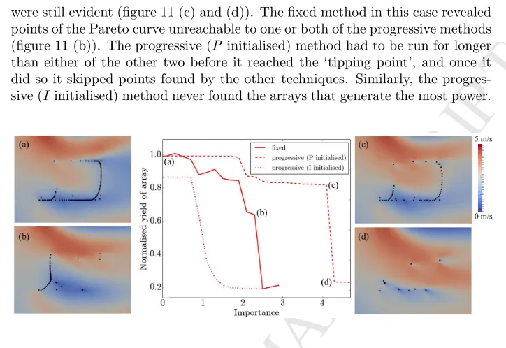
R
IP
T
A
C
C
E
P
T
E
D
The fixed starting point method was utilised first. The initial optimisation was run with ι = 0, thus optimising for P alone, and ι was increased in
in-450
crements of 0.2 until it reached 3.4, utilising the same initial array layout each time. This results in turbines whose wakes cross the ecodomain moving so that their wakes lie outside it. Turbines are also moved upstream and the number of complete barrages falls to one. Asιincreases the turbines cluster at the far end of the site from the ecodomain, and most of the turbines are placed directly on
455
top of each other (figure 6). This behaviour is a consequence of not employing minimum distance constraints, and can be viewed as an attempt by the optimi-sation to reduceI by lowering the number of turbines in the domain.
Figure 6: Yield of array, left axis, and average change of ecodomain speed, right axis, against the importance of the impact penalty. Optimised arrays with importance values of (a) 0, (b) 1, and (c) 2.2 are shown on the flow field (ms−1
). As importance is increased the turbines are moved upstream and clustered together. The ecodomain is outlined in black. Arrays all contain 32 turbines which can be placed on top of each other as in (c). Power is normalised to the yield of the array withι= 0, so that a value of 1 represents the best possible yield for an array in that location.
As ι is increased both the power produced by the array and the change in
460
the flow speed across the ecodomain decrease (figure 6). This plot, which is a representation of the Pareto curve, is a good demonstration that I is having the desired effect. The flow across the ecodomain is brought back towards its ambient state of 2 ms−1. This change initially happens quickly as turbines are
moved out of the areas closest to the ecodomain, then slows as benefits to I
465
M
A
N
U
S
C
R
IP
T
A
C
C
E
P
T
E
D
A‘tipping point’ in ι is found after which it becomes much more
advanta-470
geous to focus onI overP and the turbines are very quickly clustered together at the back of the farm, preserving the ecodomain but producing minimal power. Figure 6 shows arrays both before, (a) and (b), and after, (c), this tipping point.
The experiment was repeated twice using the progressive method outlined
475
in Section 4.2, once increasingιfrom 0 (initially emphasising P) and once de-creasing ι from 3.4 (initially emphasising I). In terms of the values of P and
I, the progressive methods produced similar results to the fixed method and in fewer iterations, but both times took longer to reach the tipping point (figure 7). This revealed additional Pareto optimal points that, due to the shape of
480
the fronts, were likely unreachable from the initial starting point previously, but became reachable when starting from a location so nearby. The iteration numbers were lower on average for the progressive techniques, with an average of 76 iterations per optimisation for progressive (P initialised) and an average of 44 iterations for progressive (I initialised). This compares to an average of
485
134 when the starting point was fixed. The number of iterations was capped at 150.
Figure 7:Comparison of array yield againstimportancewhen starting each optimisation from the same initial array layout (fixed), and when starting from the final array of the previous optimisation (progressive), initialised with an array optimised either for power or impact. The array design at the top of the tipping point is shown for each method on the flow field (ms−1
M
A
N
U
S
C
R
IP
T
A
C
C
E
P
T
E
D
The path of the solution to the progressive optimisaton can be mapped ex-plicitly as it travels through the solution space. This is seen in figure 8, in which
490
the solution to the progressive (P initialised) optimisation is mapped, with each successive optimisation represented by a different colour. It can be seen both how the solution moves from one iteration to the next within a single optimisa-tion, and also how it is translated as the weights are changed. This is the first indication of the shape of the Pareto front. The solution can be seen moving
495
from its starting pointx0, the regular grid, with no regard toI but with steadily
increasingP to its first Pareto point, xp, which represents an array optimised
forP alone. The solution can then be seen moving from one Pareto point to the next, tracing out the shape of the curve. Initially P is maintained while
I is visibly reduced. Pointsxt1 andxt2 show the starting and finishing points
500
of the optimisation that occurs over the ‘tipping point’, where I can only be further reduced with great concessions onP. The concave nature of the path over the ‘tipping point’ suggests that the front itself here is concave and that these Pareto points cannot be found due to the use of linear scalarisation.
[image:19.612.193.399.323.536.2]505
Figure 8: Tracing the solution through the solution space for the progressive starting point technique, from the starting pointx0, to an array maximised purely for power, xp and along the Pareto Front, with each change of colour representing a successive
optimisation with increased importance. xt1 and xt2 show the start and end points
of the optimisation that covers the ‘tipping point’. Power is normalised to the yield of the array withι= 0, so that a value of 1 represents the best possible yield for an array in that location.
M
A
N
U
S
C
R
IP
T
A
C
C
E
P
T
E
D
trade off that exists between power and preservation of the ecodomain is now
510
evident (figure 9). In this scenario it is possible to reduceI by almost half with-out a great compromise toP. After this the tipping point is reached causing a sharp drop in array yield so it can be safely assumed that the arrays in this area would not be of interest to developers. This confirms that the array formations of most interest have been captured.
515
Figure 9: The best estimation of the Pareto curve. A combination of Pareto points found through the three different search techniques, starting each optimisation from the same initial array layout (fixed), and starting from the final array of the previous optimisation (progressive), initialised with an array optimised either for power or im-pact. Paths are traced across the ‘tipping point’ for both progressive techniques, with sections the curve known not to lie on the Pareto front faded out. Power is normalised to the yield of the array withι= 0, so that a value of 1 represents the best possible yield for an array in that location.
For some of the points found, bothP andI are lower than for other points. This then means that these points are not truly Pareto optimal and represent only local optima within the solution space. This is a consequence that was expected when gradient based optimisation was chosen, and it could be that all
520
solutions are local optima only. There is reassurance that even if this were the case, the local solutions found are indeed close to the global optima sought as the three search techniques used all reveal solutions very close to each other. There are no points found that lie far beyond, or show significant improvement to, the other points of the curve.
525
M
A
N
U
S
C
R
IP
T
A
C
C
E
P
T
E
D
of success in any given scenario.
530
6. Case study: idealised Pentland Firth
OpenTidalFarm was run on an array of 120 turbines in an idealised repre-sentation of the Inner Sound of Stroma in the Pentland Firth, Scotland. The domain was 8.3 km by 7.8 km, with the 1.1 km by 0.7 km farm site located in the centre of the inner sound (figure 10 (a)). Inflow was from the west at a constant
535
speed of 2 ms−1
, giving a characteristic velocity of∼5ms−1
in the region of in-terest. Mesh resolution was 10m within the farm, with a steady increase toward the mesh edges. Therefore eddy viscosity was set toν = 60 m2
s−1
in order to bring grid Reynolds numbers down to O(1) and to achieve stability to a steady state on the mesh employed. All other parameters were the same as in Section 5.
540
An initial optimisation was run for power alone. The resulting array reduced flow through it by up to 2.7 ms−1and increased the flow around it by up to 3.5
ms−1(figure 10 (c)). A 1 km by 1.56 km ecodomain was identified based on the
area of greatest increase in flow.
545
Figure 10: (a) the domain used in the Pentland Firth example, (b) the ambient flow without the presence of a tidal array and (c) the change in flow after the introduction of an array optimised for power, with the ecodomain outlined in black.
As with the simple channel the solution space was explored with both the fixed and the progressive techniques, each revealing different areas of the Pareto front. The average iteration numbers were again lower for both progressive (P
initialised), 108, and progressive (I initialised), 81, than for the fixed method in
550
which all simulations ran for 150 iterations, the maximum allowed. The impact functional again reduced changes to the flow velocity within the ecodomin by moving ‘barrages’ upstream (figure 11 (a) and (b)), clustering turbines together, and eventually placing them on top of each other (figure 11 (d)).
555
M
A
N
U
S
C
R
IP
T
A
C
C
E
P
T
E
D
were still evident (figure 11 (c) and (d)). The fixed method in this case revealed points of the Pareto curve unreachable to one or both of the progressive methods
560
(figure 11 (b)). The progressive (P initialised) method had to be run for longer than either of the other two before it reached the ‘tipping point’, and once it did so it skipped points found by the other techniques. Similarly, the progres-sive (I initialised) method never found the arrays that generate the most power.
[image:22.612.126.488.123.372.2]565
Figure 11:Comparison of array yield against importance for the three search techniques of starting each optimisation from the same initial array layout (fixed), and starting from the final array of the previous optimisation (progressive), initialised with an array optimised for either power or impact. Four array designs are shown mapped on the flow field (ms−1
). (a) and (b) show ways in which array formation can change in order to reduce impact. (c) and (d) show how array formation can suddenly change at a tipping point. Arrays all contain 120 turbines which can be placed on top of each other as in (d). Power is normalised to the yield of the array withι= 0, so that a value of 1 represents the best possible yield for an array in that location.
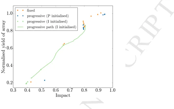
The final estimate of the Pareto curve was found (figure 12). As before there were sections of the Pareto curve, represented by the tipping points in figure 11, that are likely unreachable due to their concave nature. These were again estimated by tracing the paths of the progressive methods past them. The pro-gressive (P initialised) method eventually landed on points clearly far from the
570
Pareto front, getting ‘stuck’ in a local maxima. Its path was left off the graph as it did not provide any further information on the shape of the Pareto front.
Through utilising the three techniques an accurate picture of the Pareto front can be built, and the points from the different techniques used to validate
575
each other. Points that are shown to be sub-optimal (for example the blue ‘progressive (P initialised)’ point at the bottom of figure 12) can be ignored. After discarding such points, no further points on the curve were found to show significant improvements over the other points. Therefore, as before, finding no evidence to suggest that the points on the front are far from being global
580
M
A
N
U
S
C
R
IP
T
A
C
C
E
P
T
[image:23.612.199.502.155.345.2]E
D
Figure 12: The best estimation of the Pareto curve, combining points found through starting each optimisation from the same initial array layout (fixed), and through starting from the final array of the previous optimisation (progressive), initialised with an array optimised either for power or impact. Paths are traced across the ‘tipping point’ for the progressive (I initialised) method. Power is normalised to the yield of the array withι= 0, so that a value of 1 represents the best possible yield for an array in that location.
The major benefit of using OpenTidalFarm over other optimisation tools is that it finds Pareto optimal solutions in a relatively low number of iterations. This is demonstrated here in that it allows a greater number of Pareto points
585
to be found resulting in a clearer picture of the Pareto front. White et al [16] in 2012 investigated the trade-off between offshore wind farm development (both extent and shape of arrays), fishing industries and the whale watching sector. They used a Monte Carlo simulation that tested out different wind farm de-signs (combined with a tabu search list that ensured that each successive array
590
formation was similar to the last), performing 10,000 evaluations each time it was run on a different initial array. This method is computationally expensive due to the high number of simulations that are necessitated by the inability of Monte Carlo to find solutions guaranteed to be Pareto optimal. In a different study Lester et al [15], when investigating the trade off between fishery yield and
595
biomass preservation in marine reserves, performed 300 evaluations of randomly designed marine reserve networks, and traced out an approximate Pareto curve from the resulting plot.
The technique used here requires only a small number of simulations (∼20)
600
M
A
N
U
S
C
R
IP
T
A
C
C
E
P
T
E
D
reduce this to around 30 through utilising the ‘continuous optimisation’ function of OpenTidalFarm [33] that lets represents the entire farm as a single friction function to be optimised, the total friction of the farm acting as a proxy for the
605
number of turbines within it.
7. Conclusions
This paper demonstrates the first attempt to fully capture trade-offs between conflicting societal objectives within the tidal-turbine array design problem. The novel methodology used poses the problem as a multi-objective
optimisa-610
tion problem, in which the Pareto front is found through solving a series of gradient-based optimisation problems. Idealised problems and a demonstrative objective function are successfully used to verify the approach.
OpenTidalFarm is adapted to solve multi-objective optimisation problems
615
and used to investigate the trade-off between the conflicting objectives of max-imising power production and minmax-imising impact upon the flow regime of a tidal-stream turbine array. This is achieved through the use of a relatively simple impact functional that measures the change in the flow velocity over a user specified ecodomain. The solution space of possible array formations
620
is investigated thoroughly, and the Pareto front of optimal solutions is found. The methods discussed can be applied to similarly assess any measure of en-vironmental impact, or any societal objective, that is quantifiable and can be expressed mathematically.
625
For the objectives chosen here, the solution space is successfully explored and trade-offs successfully identified. Sections 5 and 6 show that array formations can be found that reduce impact on flow velocities without great reductions in power, but that a trade-off does exists. The extent to which the ecodomain is preserved relates to the final array design, with turbines often moving into less
630
advantageous locations (regarding yield) in order to minimise their impact. It is unrealistic to expect a tidal turbine array to produce a viable amount of power and simultaneously have no effect on the flow, and there reaches a point where the effects cannot be reduced further without a significant loss of power (figure 7). From a developer’s point of view array yield would be of utmost importance
635
and so understanding trade-offs such as this are vital.
One way to further explore any such trade-off would be to allow the number of turbines in the array to vary, letting the optimisation choose the optimal number of turbines needed to solve the problem. This would create a larger
640
solution space and could potentially reveal previously hidden solutions that are ‘more optimal’ than those found here. Culley et al [40] demonstrated this by optimising for turbine number, with each iteration requiring an ‘inner’ optimi-sation that determined the optimal array formation for that number of turbines. This approach is computationally expensive, but OpenTidalFarm’s ‘continuous
M
A
N
U
S
C
R
IP
T
A
C
C
E
P
T
E
D
optimisation’ [33] is a cheap alternative that will be utilised in future work.
The benefits of using OpenTidalFarm for any such multi-objective optimi-sation problem are well demonstrated here, as it allows us to quickly find the Pareto optimal solutions required. This happens faster than in similar work
650
which, through Monte Carlo or genetic algorithms, find optimal formations of wind turbine arrays in tens of thousands of iterations as opposed to order one hundred [16, 23]. The solution space can then be explored in a number of differ-ent ways (Section 5), and the Pareto front can be found. In other work this is achieved through the use of a Monte Carlo method ,which is not guaranteed to
655
find optimal solutions, and the shape of the front is estimated from the solutions found [15].
Once the Pareto front has been found for the problem posed, it is not pos-sible to immediately pinpoint a ‘best solution’, although intuition may at times
660
indicate one. Such a solution could only be found through a discussion with the stakeholders involved in the creation of a tidal farm in that location. This paper demonstrates the capability to provide information that would help such stakeholders find the solution that best suits them.
665
There is great scope to extend this work further, and the techniques demon-strated can be used to look at, for example, specific environmental concerns that stem from impacting upon regional hydrodynamics. Examples include habitat destruction or alteration, and change to the sediment flow, and this could be performed in realistic domains with real array sites. The hydrodynamic model
670
could also be extended to time-dependent problems to give a more accurate representation of the changes made by the array, albeit at increased expense. Beyond this, the continuous approach discussed would reduce computational time, allowing larger domains including multiple arrays to be considered, as well as providing information on the relationship between array size and
im-675
pact, furthering the understanding of any trade-off under consideration.
In this work, both the parameters used for modelling turbines and the penalty used to define an ‘impact’ objective are arbitrary. This allowed for a simple demonstration of the method on idealised scenarios. In follow-up work
680
the penalty function is replaced with a habitat suitability model, demonstrating a specific trade-off that can be investigated with the proposed method.
8. Acknowledgements
The authors would like to acknowledge Imperial College London and the Natural Environment Research Council for a Doctoral Training Partnership
685
M
A
N
U
S
C
R
IP
T
A
C
C
E
P
T
E
D
Bibliography 690
[1] Carbon Trust. Accelerating Marine Energy. Technical report, Carbon Trust, 2011.
[2] S.W. Funke, P.E. Farrell, and M.D. Piggott. Tidal turbine array optimisa-tion using the adjoint approach. Renewable Energy, 63:658–673, 2014. [3] R. Martin-Short, J. Hill, S.C. Kramer, A. Avdis, P.A. Allison, and M.D.
695
Piggott. Tidal resource extraction in the Pentland Firth, UK: Potential im-pacts on flow regime and sediment transport in the Inner Sound of Stroma.
Renewable Energy, 76:596–607, 2013.
[4] Robert Gordon University. A scoping study for an environmental impact field programme in tidal current energy. Technical report, Robert Gordon
700
University Centre for Environmental Engineering and Sustainable Energy, 2002.
[5] S.P. Neill, J.R. Jordan, and S.J. Couch. Impact of TEC arrays on the dynamics of headland sand banks. Renewable Energy, 37:387–397, 2012. [6] J.T.F. Zimmerman. The tidal whirlpool: a review of horizontal dispersion
705
by tidal and residual currents.Netherland Journal of Sea Research, 20:133– 154, 1986.
[7] M.A. Shields, D.K. Woolf, E.P.M. Grist, S.A. Kerr, A.C. Jackson, R.E. Har-ris, M.C. Bell, R. Beharie, A. Want, E. Osalusi, S.W. Gibb, and J. Side. Marine renewable energy: The ecological implications of altering the
hy-710
drodynamics of the marine environment. Ocean & Coastal Management, 54:2–9, 2011.
[8] J.E. Eckman, C.H. Peterson, and J.A. Cahalan. Effects of flow speed, turbulence, and orientation on growth of juvenile bay scallops Argopecten irradiansconcentricus (Say). Journal of Experimental Marine Biology and
715
Ecology, 132:123–140, 1989.
[9] B. Worm, E.B. Barbier, N. Beaumont, J.E. Duffy, C. Folke, B.S. Halpern, Jeremy B.C. Jackson, H.K. Lotze, F. Micheli, S.R. Palumbi, E. Sala, K.A. Selkoe, J.J. Stachowicz, and R. Watson. Impacts of biodiversity loss on ocean ecosystem services. Science, 314:787–790, 2006.
720
[10] S.W. Funke. The automation of PDE-constrained optimisation and its ap-plications. PhD thesis, Imperial College London, 2012.
[11] D.M. Culley, S.W. Funke, S.C. Kramer, and M.D. Piggott. Integration of cost modelling within the micro-siting design optimisation of tidal turbine arrays. Renewable Energy, 85:215–227, 2016.
725
M
A
N
U
S
C
R
IP
T
A
C
C
E
P
T
E
D
[13] C. Garret and P. Cummins. Limits to tidal current power. Renewable Energy, 33:2485–2490, 2008.
730
[14] M.G. Gebreslassie, G.R. Tabor, and M.R. Belmont. Investigation of the performance of a staggered configuration of tidal turbines using cfd. Re-newable Energy, 80:690–698, 2015.
[15] S.E. Lester, C. Costello, B.S. Halpern, S.D. Gaines, C. White, and J.A. Barth. Evaluating tradeoffs among ecosystem services to inform marine
735
spacial planning. Marine Policy, 38:80–89, 2013.
[16] C. White, B.S. Halpern, and C.V. Kappel. Ecosystem service tradeoff analysis reveals the value of marine spatial planning for multiple ocean uses. Proceedings of the National Academy of Sciences of the United States of America, 2012.
740
[17] R.T. Marler and J.S. Arora. Survey of multi-objective optimization methods for engineering. Structural and Multidisciplinary Optimization, 26(6):369–395, 2004.
[18] K.V. Moffaert, M.M. Drugan, and A. Nowe. Scalarized multi-objective rienforcement learning: Novel design techniques. Proceedings of Adaptive
745
Dynamic Programming and Reinforcement Learning (ADPRL), pages 191– 199, 2013.
[19] Y. Jin. Advanced Fuzzy Systems Design and Applications. Physica-Verlag, 2003.
[20] D.M. Culley, S.W. Funke, S.C. Kramer, and M.D. Piggott. A hierarchy of
750
approaches for the optimal design of turbine farms. In 5th International Conference on Ocean Energy, 2014.
[21] H.S. Huang. Distributed genetic algorithm for optimization of wind farm annual profits. Intelligent Systems Applications to Power Systems, 2007. [22] S.A. Grady, M.Y. Hussaini, and M.M. Abdullah. Placement of wind
tur-755
bines using genetic algorithms. Renewable Energy, 2003.
[23] M. Bilbao and E. Alba. Simulated annealing for optimization of wind farm annual profit. In Logistics and Industrial Informatics 2nd International Conference, 2009.
[24] G. Rudolph. Convergence of evolutionary algorithms in general search
760
spaces. Proceedings of IEEE International Conference, 1966.
[25] R.H.J. Willden, T. Nishino, and J. Schluntz. Tidal stream energy: Design-ing for blockage. In 3rd Oxford Tidal Energy Workshop, 2014.
[26] A. Scotti. Large eddy simulation in the ocean. International Journal of Computational Fluid Dynamics, 2010.
M
A
N
U
S
C
R
IP
T
A
C
C
E
P
T
E
D
[27] M. Ilicak, A.J. Adcroft, S.M. Griffies, and R.W. Hallberg. Spurious dia-neutral mixing and the role of momentum closure. Ocean Modelling, 2012. [28] S. Griffies. Science of ocean climate models.Elements of Physical
Oceanog-raphy, 2004.
[29] S. Zhao and Y.J. Liu. Spurious dianeutral mixing in a global ocean model
770
using spherical centroidal voronoi tessellations.Journal of Ocean University of China, 2016.
[30] P. Mycek, G. Gaurier, G. Germain, G. Pinon, and E Rivoalen. Experi-mental study of the turbulence intensity effects on marine current turbines behaviour. part i: One single turbine.Renewable Energy, 66:729–746, 2014.
775
[31] P. Mycek, G. Gaurier, G. Germain, G. Pinon, and E Rivoalen. Experi-mental study of the turbulence intensity effects on marine current turbines behaviour. part ii: Two interacting turbines. Renewable Energy, 68:876– 892, 2014.
[32] T. Blackmore, W. M. J. Batten, and A. S. Bahaj. Influence of turbulence on
780
the wake of a marine current turbine simulator.Proceedings of the Royal So-ciety A: Mathematical, Physical and Engineering Sciences, 470(20140331), 2014.
[33] S.W. Funke, S.C. Kramer, and M.D. Piggott. Design optimisation and resource assessment for tidal-stream renewable energy farms using a new
785
continuous turbine approach. Renewable Energy, 99:1046–1061, 2016. [34] A. Abolghasemi, M.D. Piggott, J. Spinneken, A. Vir, C.J. Cotter, and
S. Crammond. Simulating tidal turbines with mesh optimisation and rans turbulence models. Journal of Fluids and Structures, 2016.
[35] A. Abolghasemi, M.D. Piggott, and S. C. Kramer. An investigation into the
790
accuracy of the depth-averaging used in tidal turbine array optimisation.
RRenewable Energy (submitted), 2016.
[36] C.T. Jacobs, M.D. Piggott, S.C. Kramer, and S.W. Funke. On the validity of tidal turbine array configurations obtained from steady-state adjoint optimisation.VII European Congress on Computational Methods in Applied
795
Sciences and Engineering, 2016.
[37] S.C. Kramer, S.W. Funke, and M.D. Piggott. A continuous approach for the optimisation of tidal turbine farms. European Wave and Tidal Energy Conference, 2015.
[38] Z. Jiang and M. Gu. Optimization of a fender structure for the
crashwor-800
thiness design. Materials and Design, 2009.
M
A
N
U
S
C
R
IP
T
A
C
C
E
P
T
E
D
[40] D.M. Culley, S.W. Funke, S.C. Kramer, and M.D. Piggott. A surrogate-assisted aproach for optimising the size of tidal turbine arrays. Submitted to Renewable Energy, 2016.
M
A
N
U
S
C
R
IP
T
A
C
C
E
P
T
E
D
Research Highlights
===================
Maximising power while minimising impact posed as multi-objective optimisa-tion.
Gradient-based optimisation to find optimal solutions quickly and efficiently.
Turbine arrays that reduce impact on the flow regime with minimal change in power.
Pareto front of optimal solutions explored and trade-off characterised.