Discovering a Domain Knowledge Representation for Image Grouping: Multimodal Data Modeling, Fusion, and Interactive Learning

(1)

Rochester Institute of Technology

RIT Scholar Works

Theses Thesis/Dissertation Collections

8-2017

Discovering a Domain Knowledge Representation

for Image Grouping: Multimodal Data Modeling,

Fusion, and Interactive Learning

Xuan Guo

[email protected]

Follow this and additional works at:http://scholarworks.rit.edu/theses

Recommended Citation

(2)

Discovering a Domain Knowledge Representation for

Image Grouping: Multimodal Data Modeling, Fusion,

and Interactive Learning

by

Xuan Guo, B.S.

DISSERTATION

A Dissertation Submitted in Partial Fulfillment of the

Requirements for the Degree of Doctor of Philosophy

in the B. Thomas Golisano College of

Computing and Information Sciences

Rochester Institute of Technology

Rochester, NY

(3)

Discovering a Domain Knowledge Representation for

Image Grouping: Multimodal Data Modeling,

Fusion, and Interactive Learning

by

Xuan Guo

Committee Approval:

We, the undersigned committee members, certify that we have advised and/or

supervised the candidate on the work described in this dissertation. We further certify that we have reviewed the dissertation manuscript and approve it in partial fulfillment of the requirements of the degree of Doctor of Philosophy in Computing and Information Sciences.

______________________________________________________________________________

Prof. Anne R. Haake Date

Dissertation Co-advisor

______________________________________________________________________________

Prof. Qi Yu Date

Dissertation Co-advisor

______________________________________________________________________________

Prof. Cecilia Ovesdotter Alm Date

Dissertation Committee

______________________________________________________________________________

Prof. Rui Li Date

______________________________________________________________________________

Prof. Pengcheng Shi Date

______________________________________________________________________________

Prof. Daniel Phillips Date

Dissertation Defense Chairperson

(4)

Abstract

Discovering a Domain Knowledge Representation for

Image Grouping: Multimodal Data Modeling, Fusion,

and Interactive Learning

Publication No.

Xuan Guo, Ph.D.

Rochester Institute of Technology, 2017

Supervisors: Dr. Anne R. Haake Dr. Qi Yu

In visually-oriented specialized medical domains such as dermatology

and radiology, physicians explore interesting image cases from medical

im-age repositories for comparative case studies to aid clinical diagnoses, educate

medical trainees, and support medical research. However, general image

clas-sification and retrieval approaches fail in grouping medical images from the

physicians’ viewpoint. This is because fully-automated learning techniques

cannot yet bridge the gap between image features and domain-specific

con-tent for the absence of expert knowledge. Understanding how experts get

(5)

As a prior study, we conducted data elicitation experiments, where

physicians were instructed to inspect each medical image towards a

diagno-sis while describing image content to a student seated nearby. Experts’ eye

movements and their verbal descriptions of the image content were recorded

to capture various aspects of expert image understanding. This dissertation

aims at an intuitive approach to extracting expert knowledge, which is to find

patterns in expert data elicited from image-based diagnoses. These patterns

are useful to understand both the characteristics of the medical images and

the experts’ cognitive reasoning processes.

The transformation from the viewed raw image features to

interpre-tation as domain-specific concepts requires experts’ domain knowledge and

cognitive reasoning. This dissertation also approximates this transformation

using a matrix factorization-based framework, which helps project multiple

expert-derived data modalities to high-level abstractions.

To combine additional expert interventions with computational

pro-cessing capabilities, an interactive machine learning paradigm is developed to

treat experts as an integral part of the learning process. Specifically, experts

refine medical image groups presented by the learned model locally, to

incre-mentally re-learn the model globally. This paradigm avoids the onerous expert

annotations for model training, while aligning the learned model with experts’

(6)

Acknowledgments

I would like to express the deepest appreciation to my advisors, Profs.

Anne R. Haake and Qi Yu, for the support, encouragement, inspiration and

guidance they provided me throughout my PhD study and life.

I am grateful to my dissertation committee: Profs. Cecilia Ovesdotter

Alm, Rui Li, and Pengcheng Shi for their insightful comments.

My appreciation goes to my colleagues and good friends Jingjia Xu,

Wenbo Wang, Tong Liu, Mohamed Elshrif, Jwala Dhamala, Ruslan Dautov,

Katy Tarrit, Preethi Vaidyanathan, and Dong Wang for their priceless presence

and support.

Lastly, I would like to express my gratitude to my dear parents for their

support, love, presence and patience.

The work presented in this dissertation is supported by grants from the

(7)

List of Tables

1.1 Two types of thought units. . . 4

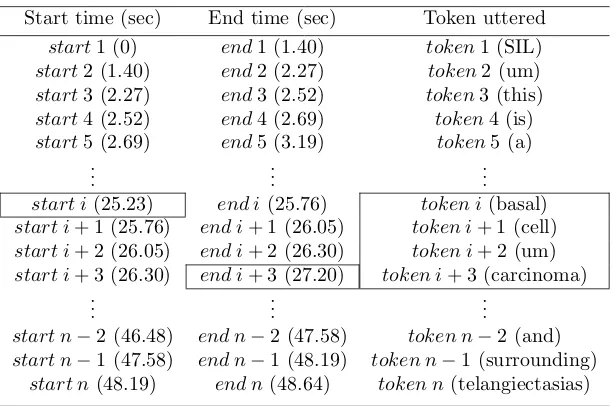
3.1 A diagnostic narrative corresponding to Figure 1.1 with time stamps and tokens. There is a multiword expression (basal cell carcinoma) boxed in the middle rows. . . 62

3.2 An illustration of the narrative in Table 3.1 after the detection of a medical multiword expression, basal cell carcinoma. . . 63

3.3 Narrative clustering performance. . . 74

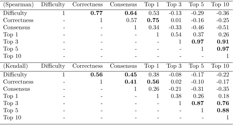
3.4 Correlation among different image rankings based on the Spear-man and Kendall methods, respectively. . . 82

3.5 Narrative correctness classification performances. The positive class for ROC is high-correctness. . . 95

3.6 Ranked features by random forest classifier. . . 95

4.1 Precision (P) and Recall (R) comparison at lesion morphology level. Among 48 images in the database, there are 9 images considered as containing the morphology macule, 38 papule, 5 bulla, 4pustule, and 1 nodule. . . 114

4.2 Precision (P) and Recall (R) comparison at lesion morphology level for the additional test that involve more images in the database. . . 115

4.3 Clustering performance by eye tracking data. . . 121

4.4 Clustering performance by verbal data. . . 121

4.5 Clustering performance by multimodal data. . . 121

5.1 Image grouping performances of fully automated learning and our paradigm. . . 144

5.2 The percentage of images in the reference list to appear within the top 10 retrieved neighbors . . . 145

5.3 The percentage of images in the reference list to appear within the top 15 retrieved neighbors . . . 145

(11)

List of Figures

1.1 Left: One medical image case used in the study (diagnosed as basal cell carcinoma; image courtesy of Dr. Cara Calvelli),

Right: image inspection, audio recording, and eye tracking. . . 3

1.2 The example eye gaze data instance (a) and a diagnostic nar-rative annotated by thought unit labels (b) that correspond to the same image. . . 4

1.3 Connections between chapters in this dissertation. . . 9

2.1 The term-term interaction graph computed using the semantic relatedness score in UMLS (details in Section 3.4.2). The ver-tices represent terms and edges the relatedness scores between terms. . . 42

2.2 Probabilistic latent semantic analysis. . . 45

2.3 Latent Dirichlet allocation. . . 46

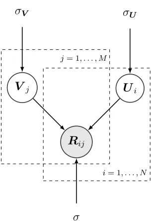
2.4 Graphical illustration of PMF. . . 49

2.5 Relationships between representation learning models in the framework of matrix factorization. . . 50

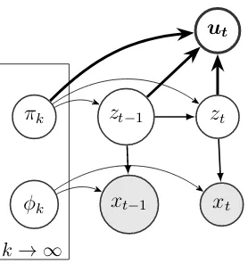
2.6 The hierarchical Dirichlet process-hidden Markov model that learns from a single observation sequence {xt}t=1,2,···,T. . . 53

2.7 Integrating outπ. For simplicity, the global measureGis omitted. 55 2.8 The auxiliary variables u depends on z and π. . . 58

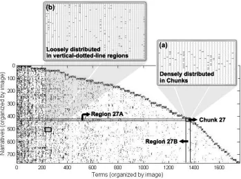
3.1 The narrative-term matrix with tf-idf scores is organized by image. The zero scores are plotted in white and others in dark grey. . . 65

3.2 An analysis of the occurrence of medical terms in narratives and distribution across images. . . 67

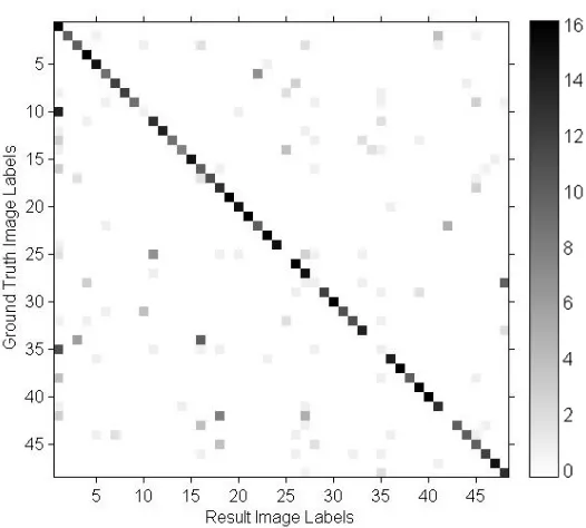
3.3 Confusion matrix of clustering results based on the anchor con-cept algorithm. The darkness of a block indicates the number of narratives that are in this block. . . 73

(12)

3.5 The correctness score distribution across all narratives. . . 85 3.6 The self-reported diagnostic confidence score distribution across

all narratives. . . 85 3.7 The hierarchical Dirichlet process-hidden Markov model that

learns from multiple narratives as a group. . . 86 3.8 Normalized state transitions in narrative groups regarding

diag-nostic correctness. One salient transition to discriminate both groups is from pattern 4 (the 4th _{row) to 1 (the 1}st _{column). .} ₉₀

3.9 The correctness score distributions between the narratives with state transition (4→1) and those without. . . 90 3.10 Two narration patterns learned from all narratives in

Exper-iment I. Top 20 terms of each pattern are visualized through word cloud in which the font size indicates term frequency. Each table presents the thought unit (TU) proportion of the pattern. 91 3.11 Meaningful patterns discovered from diagnostic confidence study

in Experiment II. . . 91 3.12 Normalized state transitions in narrative groups regarding

di-agnostic confidence. Group (a) possesses slightly more self-transitions of 1, 5, 10 and 11 than group (b). . . 92 3.13 Two narration patterns learned from all narratives in

Experi-ment II. Word cloud shows top terms of each pattern. . . 92 3.14 Example narratives in the diagnostic correctness study. . . 94

4.1 A symmetrical viewing pattern detected by GMM in eye fixations.103 4.2 A solitary viewing pattern detected by GMM in eye fixations. 104 4.3 An overview of system design (user view). . . 106 4.4 An overview of system design (system view). . . 107 4.5 Using the end user’s and physicians’ eye movements as filters

for visual features to retrieve images. . . 110 4.6 Fusing multiple data modalities. Coefficient matrix, C, and

basis matrices,P and Q, are learned from an eye tracking data matrix, E, and a verbal description data matrix, V. . . 118 4.7 Confusion matrix of clustering trials by image based on

(13)

4.9 A template lesion of papule is derived from an eye fixated papule. This template can be used to detect visually similar lesions in the image. . . 127

5.1 Overview of the flow chart of our expert-in-the-loop paradigm. An expert encodes domain knowledge as special constraints through rounds of interactions. . . 132 5.2 Image grouping interface. . . 133 5.3 Image groupings generated using subsets of features. . . 134 5.4 An example of the visualization in popup window after the user

(14)

List of Algorithms

1 Projected gradient method [1] . . . 28

2 Alternating non-negative least square [2] . . . 28

3 Multiplicative rules for Euclidean distance [3] . . . 29

4 Multiplicative rules for KL-divergence [3] . . . 29

5 Feature-sign search algorithm (for each data instance xj) [4] . 35 6 A modified feature-sign search algorithm for GrNMF [5] . . . 39

7 The forward algorithm . . . 52

8 The backward algorithm . . . 52

9 The forward-backward algorithm . . . 52

(15)

Chapter 1

Introduction

1.1

Background

In visually-oriented specialized medical domains such as dermatology and

ra-diology, physicians need to study and compare medical image cases to aid

clinical diagnoses, support medical research, and educate medical trainees.

This can be aided by computational systems that organize medical images

according to the physicians’ understanding of the image content. This

dis-sertation proposes to understand the medical images from the perspective of

experts’ domain knowledge.

Since medical knowledge tends to be tacit and difficult to convey and

obtain, medical training usually takes years of internships and specialized

res-idencies. Medical training will benefit from approaches that can properly

represent and visualize expert knowledge. This dissertation develops

vari-ous representation learning strategies to extract expert knowledge from

mul-timodal datasets collected from physicians when they inspect medical images.

The datasets were constructed by the Human-Centric Multi-Modal Modeling

(16)

dermato-logical images (courtesy of Logical Images, Inc.) as visual stimuli. The images

in Experiment I represent a wide range of dermatology diagnoses [6], whereas

those in Experiment II focus on more examples of a few diagnoses.

Dermatol-ogy was chosen as a testbed, as it is a visually-based medical specialty that

requires specific, complex perceptual expertise. Following a modified

master-apprentice approach [7], each participating physician was asked to describe the

visual content of each image aloud, as if teaching a student who was seated

nearby [8]. The physicians’ speech and eye movements were recorded during

the experiments. These experiments were approved by Rochester Institute

of Technology’s Institutional Review Board, and all participants provided

in-formed consent before participating in the experiments.

The approach to gathering expert data during image inspection

effec-tively traces how experts use their knowledge for image-based problem solving.

This is because this approach involves a more natural task for physicians to

perform in contrast to asking them to conform to predefined image annotation

labels and rules. Figure 1.1 presents one of the images, and the experimental

setup. Figure 1.2 contains one corresponding eye tracking data instance and

diagnostic narrative transcribed from physicians’ spoken descriptions. Similar

to this example, all the spoken narratives were comprehensively transcribed

with sequences of words labeled by time stamps using the speech analysis tool

Praat [9]. Overall, the datasets comprise 1670 transcribed spoken narratives

and the same number of eye tracking trials.

(17)

Figure 1.1: Left: One medical image case used in the study (diagnosed asbasal cell carcinoma; image courtesy of Dr. Cara Calvelli),Right: image inspection, audio recording, and eye tracking.

-identified diagnostic thought units (TUs). These TUs cover the terminology

to standardize the description of skin lesions, including lesion arrangement,

distribution, texture, color, primary lesion type, and diagnosis [10]. For a

follow-up study of the reasoning processes of the collected diagnostic verbal

narratives, we recruited three dermatologists to evaluate the narratives from

the 16 participating physicians in Experiment I in terms of their diagnostic

correctness. A correctness score was assigned to each narrative, which balances

the correctness of described primary lesion type, differential diagnosis, and

final diagnosis. We refer to them as Type II thoughts to distinguish them (the

indirect findings) from the rest TUs that are direct findings. The identified TUs

are shown in Table 1.1, and one example annotation is in Figure 1.2-(b). In

addition to the semantic relevance, there is a temporal correspondence between

the data modalities, as both modalities of expert data were synchronously

(18)

(a) A collected gaze data instance.

(SIL) um this is a (SIL) pearly lobulated (SIL)

pink (SIL) papule with telangiectasias multi-lobulated

papule with telangiectasias (SIL) on the upper_:::: cheek_::::

(SIL) of (SIL) an elderly individual (SIL) say nodular_{. . . .}

. . . .

basal. . . .cell. . . .carcinoma it’s a . . . .nodular _{basal. . . .}_{. . . .} _{cell. . . .}carcinoma (SIL) uh (SIL) there is some surrounding_{. . . .} _{sun . . . .}_{. . .} damage

(SIL) and surrounding telangiectasias

PRI ; SEC ; LOC ; DEM ;_:::: _{DX or . . . .}_{. . .} DIF

(b) A dermatologist’s diagnostic narrative for the image. (SIL)represents silent pause.

Figure 1.2: The example eye gaze data instance (a) and a diagnostic narrative annotated by thought unit labels (b) that correspond to the same image.

Given the specialized domain, in which expert knowledge is required

to solve difficult problems (i.e., making diagnoses), the collected multimodal

expert data are ideal observations for this dissertation research to learn

repre-sentation of knowledge from human data. Besides, these datasets also reflect

the difficulty of research in the field—numerous medical images are not

an-Table 1.1: Two types of thought units.

Thought Unit Labels (Abbr.) Instances

T

yp

e

I

Patient DEMographics (DEM) elderly, caucasian, woman Body LOCation (LOC) arm, upper lip, knuckles Lesion CONfiguration (CON) linear, annular, grouped

SECondary finding (SEC) crust, ulcer, erythematous Lesion DIStribution (DIS) solitary, bilateral, extensive

T

yp

e

II PRImary lesion type (PRI) papule, plaque, patch

DIFferential diagnosis (DIF) X, Y or Z Final Diagnosis (DX) this is X

(19)

notated, meaning that we have to learn from a small annotated dataset for

knowledge that can be generally utilized. One important finding during data

collection is that the dermatology images can be difficult to inspect even for

ex-perts, because these photographic images often contain complex visual features

which may or may not be relevant to making an accurate diagnosis. Moreover,

in some cases the information in the image is not sufficient to support a final

diagnosis where the physicians requested biopsy as additional evidence. These

findings show the tight connection of the proposed research to the real-world

clinical settings and educational image uses.

1.2

Problem Definition

Eye movements provide insights into experts’ interests of the key visual

fea-tures and perceptually important regions in the images. Existing work in the

HCM3 Lab shows the correlation between image feature distribution and eye fixation arrangement [11]. These indicate the promising direction to

understand image content from expert-derived data.

Previous studies in HCM3 also include developing computational mod-eling to discover hidden visual behavioral patterns from eye movement data

[12, 13, 14]. Several distinctive types of patterns (i.e., Signature Patterns)

were discovered by a model and verified by a domain expert [15, 16]. This

indicates that it is possible to extract expert knowledge from the

collected behavioral data.

(20)

developed with domain experts in order to examine participating physicians’

diagnostic narration structure [8, 17]. A correspondence was found between

the learned eye movement patterns and the conceptual units of thought by

time-aligning the patterns with annotated narratives [12]. This finding

sug-gests another research direction taken in this dissertation; that is,

to mathematically fuse multimodal expert data for comprehensive

image understanding.

We are learning from a small dataset (compared with the large

vol-ume of medical images in the field), and the collected multimodal expert data

contain some data instances where the diagnoses are inaccurate. This makes

the outcome (e.g., the learned data representation, and the estimated

param-eters) sensitive to random variations in data (i.e., overfitting). To include

prior knowledge in the representation learning, this dissertation also aims

at developing a framework to receive additional inputs of domain

knowledge through expert interactions.

Given the elicited multimodal expert data and the promising research

directions above, the objectives of this dissertation are—(1) To build models

with the diagnostic verbal narratives for discovering expert-produced

behav-ioral and cognitive patterns. (2) To develop a framework that integrates the

features in multiple modalities for a unified data representation, which explains

the observations in these modalities and their correspondences. (3) To

imple-ment a machine learning system that allows expert manipulation of images

(21)

es-sentially inverse problems, where I discover experts’ uses of domain knowledge

and their diagnostic reasoning processes from the collected eye movements and

transcribed verbal narratives.

1.3

Dissertation Contributions

• The visual stimuli (i.e., the image content) and the expert cognitive

pro-cessing of the stimuli are interwoven. The collected expert data contain

the variances intrinsically from both the images and the experts. This

dissertation discovers interpretable behavioral patterns from expert data

and discloses both the characters of the medical images and those of the

participating experts.

• The multimodal data were collected during in-scenario experiments and

hence the data reflect different aspects of the same cognitive processes—

i.e., image-based diagnostic reasoning. In spite of the obvious semantic

relevance across data modalities, the relationship between the modalities

is hidden and needs modeled. This dissertation develops and studies a

machine learning framework that fuses multimodal expert data, so as to

recover the underlying conceptual and cognitive elements.

• The sparsity of the multimodal observations introduces an additional

challenge for accurate estimation of model parameters. The studies

in this dissertation incorporate knowledge resources as constraints in

(22)

medical knowledge resources (for representation learning) and additional

expert inputs (for interactive machine learning).

1.4

Dissertation Organization

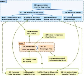
The following chapters in this dissertation are organized as follows (see

Fig-ure 1.3): Chapter 2 first introduces the background and related studies,

in-cluding the domain knowledge and visual perception in medical diagnosis, and

the idea of human computation through multimodal expert data. Chapter 2

also reviews various fundamental approaches that are used and referred to in

later chapters. Chapter 3 models the collected diagnostic verbal narratives

for medically meaningful topics. Section 3.2 presents the narrative processing

with the Unified Medical Language System (UMLS) [18] to extract medical

terms that are used for modeling and analysis in the rest of the dissertation.

Section 3.3 presents narrative clustering based on a topic modeling approach.

Section 3.4 develops two lexical metrics that are useful to explore the

at-tributes of physician groups and their diagnostic relevance based on the verbal

narratives. Section 3.5 develops a hierarchical dynamic model to recognize

the narration patterns that match physicians’ diagnostic reasoning stages and

are useful to predict diagnostic correctness. Chapter 4 reports on the

mix-ture components identified in physicians’ eye movement data that match the

medical abnormalities in the images. This finding supports two other

stud-ies in the chapter to develop a human-centered information retrieval (HCIR)

(23)

[image:23.612.136.490.124.448.2]

Figure 1.3: Connections between chapters in this dissertation.

multimodal data for a set of unified latent variables (Section 4.4). Chapter 5

describes an interactive machine learning paradigm developed for the case of

medical image grouping, where additional expert inputs can be used as

con-straints to guide the machine learning processes. Chapter 6 summarizes this

(24)

Chapter 2

Related Work

Since many medical images are inherently complex and noisy due to both

photographic inconsistency and different presentations of even the same

med-ical condition, grouping relevant medmed-ical images into semantmed-ically related and

meaningful groups has been a long-standing challenge. This chapter first lays

the theoretical foundation for research in the field of medical diagnosis in

Section 2.1, followed by describing the external language tools and multiple

human sensors from the human computation perspective (Section 2.2).

Sec-tion 2.3 then reviews the technical building blocks that can be used with the

tools and data to study expert knowledge and understand medical images.

Chapters 3, 4, and 5 use these building blocks for studies of diagnostic

reason-ing and medical image understandreason-ing, and the outcomes are useful to support

medical image grouping.

2.1

Image-based Diagnostic Reasoning

Since the content in medical images is beyond colors, textures, and shapes,

fully automated computer vision algorithms that only use low-level image

(25)

semantics and represent a medical image by a feature vector, we need to

under-stand the image content, especially the key content based on which a physician

can make a diagnosis about the image. However, the task of medical image

understanding remains challenging, because it requires domain knowledge and

perceptual expertise.

In the medical field, diagnostic reasoning processes can be explained

by two cognitive systems in thedual-process theory, namelyintuitive and

ana-lytical [19]. However, current research on medical diagnosis relies on research

interviews or clinical chart records [20], reports of clinicians [21], and

physi-cians’ response time [22], and hence overlooks much detailed information.

To contribute to both fields above, we jointly study the content in

medical images and physicians’ diagnostic decision-making. Specifically, we

collected multimodal data from physicians when they were engaged in

diag-nostic reasoning based on medical images (Section 1.1). To disentangle the

underlying factors that relate to expert interpretation of image content, In

this dissertation we model the collect data in Sections 3.3, 3.5, and 4.4. The

model outcomes help understand both physicians’ diagnostic reasoning

pro-cesses and their interpretations of image content by domain knowledge.

2.2

Conceptual Knowledge, Perceptual Expertise, and

Human Computation

The general computer vision algorithms that automatically detect semantic

(26)

se-mantics in medical images. Parsing and using the sese-mantics in medical

im-ages requires external knowledge [23]. One resource of domain knowledge is

the UMLS, which provides access to medical concepts and concept relations

in the medical domains. The domain experts constitute another knowledge

resource.

2.2.1 Unified Medical Language System

Ontology resources such as WordNet [24], VerbNet [25] and ImageNet [26] have

been used in general domains for extracting semantics in texts and images. The

UMLS can serve such a purpose in medical domains. It is a knowledge source

for medical terminology research and information retrieval [27], constituting

the largest existing semantic network of medical terms and their lexical

rela-tions [18, 28]. As an ontology of medical concepts it has been used to process

clinical records, to relate or disambiguate medical terminologies, and to serve

as a knowledge base for health care systems [18]. It has also been used to

assist feature engineering to tackle the intrinsic problem of data sparsity in

clinical texts [29, 30].

To represent expert knowledge from linguistic data, we have

prepro-cessed the data by programming with MetaMap, which is a knowledge-intensive

tool that automatically annotates biomedical text tokens by UMLS

Metathe-saurus concepts [31]. Our program first filters out the non-medical terms in

the verbal narratives, and then detects and reconstructs medical multiwords

(27)

this manner, each spoken narrative is segmented as a sequence of words and

multiword expressions, which can be used for further analysis and modeling.

2.2.2 Natural language and domain knowledge

Language is the primary conduit to express meaning. Our diagnostic verbal

image descriptions, collected during medical image inspections, form a

non-trivial corpus with different levels of language features. For example, speech

features can be used to study experts’ certainty in decision-making [32, 33, 34];

natural language can be processed and statistically analyzed at the lexical level

to reveal humans’ decision styles [35]; additionally, sense relationship can be

extracted using an ontology [36, 37]. This effort focuses on sense-based

repre-sentation as a reflection of human knowledge.

Studies in both computer vision and natural language processing use

the correspondence between image content and human annotations to reveal

semantics [38]. In natural scene image corpora, the annotations summarize the

meanings of visual content [39]. In return, the visual content in images provides

semantic context to disambiguate a lexical item (e.g., acrane as a bird vs. that

in a construction field). For example, Wu et al., defined the Flickr distance

to measure the relationship between semantic concepts (objects, scenes) in

the visual domain [40]. For each concept, a collection of images are obtained

from Flickr, and their visual characteristics are captured. Using information

in images helps capture the visual relationship between concepts. Their study

(28)

the resulting concept network is more statistically coherent to humans’ current

knowledge. There are more examples integrating verbal metadata with image

features [39]. A case of using language for characterizing the meaning of images

is shown in Li et al.’s study [41]. Using language tags of image regions, an

ontology of related concepts are introduced to achieve hierarchical annotation.

Natural language data provide multiple challenges: (1) Language is,

by nature, sparse [42]. In most linguistic data sets, the vast majority of

lex-ical items tend to occur rarely, and speakers can express similar meaning in

a variety of ways, both syntactically and lexically. (2) Semantic ambiguity

occurs in language data. The understanding and interpretation of ambiguous

language data depends on domain knowledge. (3) The difference in narration

styles among users results in variability that obscures common strategies of

diagnostic reasoning. (4) Language data are influenced by the mode in which

they were produced. Naturally occurring speech data differ substantially from

standard written text data.

Physicians in specialties such as radiology and dermatology have

de-veloped visual perceptual expertise. They better recognize domain-specific

patterns than unsupervised algorithms that lack guidance from medical

knowl-edge [13, 43]. However, it is time consuming and impractical for physicians

to manually annotate medical images since these images (1) can be stored in

large-scale image databases with a large and rapidly growing number of

dig-ital images, and (2) may reside within individual medical practices or small,

(29)

Researchers have made efforts to incorporate domain knowledge in

im-age clustering [44]. However, truly understanding physicians’ use of knowledge

(especially during image-based diagnosis) remains a challenging task, because

visual diagnostic reasoning is a complex interaction of domain knowledge,

per-ceptual expertise, reasoning processes [45], and idiosyncratic visual

informa-tion in the image case being inspected by physicians.

We elicit expert knowledge by collecting data from physicians as they

engage in medical image inspection. This approach involves a more natural

task for experts to perform in contrast to asking them to conform to predefined

image annotation labels and rules.

We exploit human experts’ knowledge to facilitate medical image

group-ing by applygroup-ing a methodology that is more objective and automated than

current research [22, 46, 47]. The intuition is that the meaning of a medical

image is expected to be mirrored by the spoken narrative of a physician when

s/he describes the image during a diagnostic process. In this way, we

incorpo-rate physicians’ domain knowledge, obtained from years of systematic study

and clinical training, to achieve more effective medical image grouping.

2.2.3 Eye tracking and visual perception

People are exposed to plenty of visual information everyday, but relatively

little of that information is processed due to our reliance on prior experience.

Humans shift the point of regard to regions requiring high resolution to gather

(30)

As a reflection of human responses to visual information, eye movements

re-veal the interaction between image features and human visual attention. It

highlights the important visual information perceived by human observers.

Eye movements can be described as a combination offixations and

sac-cades. Fixations occur when the eyes remain at a particular spatial location in

a visual stimulus, typically over a minimum duration of 100-200 milliseconds

[48]. To re-orient the eye to other locations of interest, the eye makes rapid,

ballistic movements known as saccades. Many eye tracking features/methods

have been defined based on statistical analysis of fixations and saccades in

raw data, including comparison of scanpaths [49], saliency maps [50], and

more complicated scanning patterns [12]. Although eye movements cannot

completely explain visual cognitive processes, many studies of individuals’ eye

movements, as they perform tasks, have established relationships between

vi-sual attention and cognition [51].

Eye movements are influenced by both bottom-up visual processing and

top-down search tasks and knowledge, so eye tracking opens a window to

ex-plore human visual information gathering guided by knowledge and intentions

[52]. In particular, human eye movements are a combination of visual input

and several cognitive systems, including short-term memory for previously

attended information in the current fixated position, stored long-term visual,

spatial and semantic information about other similar visual cases (knowledge),

and the goals and plans of the viewer (task) [53]. Fixations on particular parts

(31)

the structural information inherent in the image. These attributes of human

eye movements result in applications of eye tracking in various studies. For

example, Kunze et al. inferred participants’ language reading level from their

reading speed and fixation duration [54]. Human gaze has been utilized to

ex-tract regions of interest (ROIs) of an image to perform attention-based image

retrieval [55]. Visual attention has also been used as feedback in web searches

[56], for predicting salient regions of web pages [57], and to indicate different

levels of domain expertise by disclosing how experts vs. non-experts behave

visually when they are searching for task-relevant clues [58].

In vision-based complex problem-solving scenarios, such as image use,

human experts’ tacit knowledge is key to understanding and can be applied

toward enhancing computer vision algorithms. Eye tracking helps capture such

knowledge, because visual strategies are executed at a level below conscious

awareness and eye tracking is able to provide information that is not available

through methods such as introspection. Eye tracking a group of experts allows

us to study experts’ subconscious image viewing behaviors in common by

objectively measuring their eye movements.

2.3

Representation Learning Approaches

The data sparseness problem generally exists in natural language from

vari-ous domains. For example, there are a large number of distinct terms in our

dataset, because various naming preferences are used by physicians.

(32)

learning the transformations of raw data to compact and meaningful

repre-sentations. It has been successful in various domains. For example, topics

can be learned from the terms in documents [59], and levels of objects (e.g.,

edges, parts of faces, and faces) can be learned from pixels in face images [60].

Representation learning can also be applied to learn meaningful

representa-tions in audio signals and haptic data [61]. These learned new features are

usually in a more compact space and hence reduce the computational burden

of classification and prediction that follows.

Another use of representation learning is to visualize high-dimensional

data in a user panel as a low-dimensional embedding through techniques such

as multidimensional scaling (MDS) [62] and t-distributed stochastic

neighbor-hood embedding (t-SNE) [63]. This allows users to inspect, understand and

refine a large volume of data in a simple feature representation through

inter-actions.

In order to systematically arrive at a preferred representation,

repre-sentation learning essentially applies mathematical operations to the original

feature space. Constraints are usually designed in the objectives to keep only

those features that co-vary the most with respect to outcomes of interest. A

discussion of constraints can be found in Section 2.3.2. Although

representa-tion learning can be extended as a framework to include thehuman in the loop

for more preferred learning results (see Chapter 5), here we still consider it as

(33)

2.3.1 Classical models

In order to explain the general mechanisms of representation learning, we

first describe a popular data clustering technique (i.e., K-means) and two

unsupervised feature transformations (i.e.,principal component analysis [PCA]

and independent component analysis [ICA]). They were developed to learn a

new feature representation for different purposes.

K-means is a procedure to partition data set X = {x1,· · · ,xn} ⊂

Rm×ninto clustersC1,· · · , Ckbased on a specified numberk, where each data

point serves as a prototype of the cluster it belongs to.

k X

i=1

n X

j=1

zijkxj −µik

2 _(2.1)

where the indicator variablezij = (

1, if xj ∈Ci

0, otherwise.

K-means is implemented through iterative refinement—in each

itera-tion, assigning each datum to the cluster with the nearest mean (E-step) and

updating the new cluster centroids by minimizing sum of distance to all data

in cluster (M-step; minimize Eq. (2.1) w.r.t., µ). The original feature space

(cardinalitym) is consequently projected to cluster labels (cardinality 1).

Principal Component Analysisis a procedure that transforms the

original space of possibly correlated features into a space of linearly

uncorre-lated features called principal components [64]. This transformation is defined

(34)

vari-ance (i.e., it accounts for as much of the variability in the data as possible),

and each succeeding component in turn has the highest variance possible under

the constraint that it is orthogonal to (i.e., uncorrelated with) the preceding

components. To retain the useful information (i.e., most of the variability in

the data) and remove noise, the number of components is optimized resulting

in usually only the first few components in the new space being kept. PCA

generates a new representation in which the new features are not correlated.

It is often used as data whitening to compress data and speed up the following

learning process [65], or for visualization purposes [66].

PCA essentially centers the data matrixX first and then uses singular

value decomposition (SVD) to decompose X into a diagonal matrix Σof the

same dimension as X and with nonnegative diagonal elements in decreasing

order, and unitary matrices U and V such that,

Xn×m ≈Un×nΣn×nV>n×m (2.2)

where the rows ofV> are eigenvectors of the covariance matrixPX =X>X.

The matrix Σ is diagonal, with each element σii =

√

λi (the ith eigenvalue).

Rows ofU are coefficients for basis vectors in V.

The manifold hypothesis believes that the probability mass

concen-trates near regions that have a much smaller dimensionality than the original

space where the data lives [67]. In other words, the data points are

actu-ally samples from a low-dimensional manifold that is embedded in a

(35)

the underlying factors through linear transformation in order to find a

low-dimensional representation of the data.

Independent Component Analysis is a computational method to

separate a multivariate signal into independent subcomponents. ICA is a

special case of blind source separation [68]. A common example application is

thecocktail party problemof listening in on one person’s speech in a noisy room.

ICA generates a new representation in which the new features are independent

signal sources. Each feature in the original space is a combination of these new

independent features. ICA can be used to disentangle noise from the target

signal [69].

The un-correlation used in PCA is characterized by,

E[xy] =E[x]E[y] (2.3)

whereas the independence is given by,

E[f(x)g(y)] =E[f(x)]E[g(y)] (2.4)

The uncorrelation only measures linear relationship, whereas the independence

is stronger to measure the existence of any relationship.

2.3.2 Matrix factorization-based models

Matrix factorization (MF) seeks to learn a low rank approximation from

an input data matrix using two factors [59]. Suppose we have a data matrix

(36)

The goal of matrix factorization is to generate a more compact and precise

rep-resentation of the input matrixX by approximating it via the multiplication

of two factor matricesH ∈_Rn×k _and _C _∈

Rk×m.

X ≈HC (2.5)

min

H,CkX −HCk

2

F (2.6)

where the Frobenius norm k · k2

F is used to measure the error between the

original input X and its low rank approximation HC.

The matrix H (often referred to as basis matrix) can be viewed as

a dictionary, because it reveals the transformation from the original feature

space to latent variables that form a new basis. The matrixC (often referred

to ascoefficient matrix) represents the data instances by combinations of these

latent variables. The number of latent variables, k, is usually small to enforce

the low rank of both factor matrices.

Probabilistic interpretation of MF: Now assuming that the observed data

matrix can be recovered by its low-rank approximation HC with additional

Gaussian noise :

X ≈HC ⇐⇒ X−HC = (2.7)

where the is a matrix to denote the reconstruction error. The entries ij’s

are assumed to be independent and identically distributed (i.i.d.)

accord-ing to a Gaussian distribution with zero mean and variance σ2

(37)

reconstruction error). Due to the independent assumption the joint

distribu-tion of all data items factorizes:

p(X|H,C) =Y

i Y

j

N(Xij; [HC]ij, σ2r) (2.8)

=Y i Y j 1 √

2πσr

e

−1 2

X_ij−[HC]_ij σr

2!

(2.9)

Taking the logarithm yields the log-likelihood,

lnp(X|H,C) = −nmln

√

2πσr

− 1

2σ2

r X

i X

j

(Xij −[HC]ij)2

| {z }

DE(X,HC)

(2.10)

Maximum likelihood (ML) estimation: Maximizing the right hand side of Eq. (2.10) w.r.t. H and C is equivalent to minimizing the squared Euclidean distance DE(X,HC) for MF.

MF framework to explain classical representation learning models:

The framework of MF can be used to interpret the classical models in

Sec-tion 2.3.1, such as the popular data clustering technique (i.e., K-means), and

the unsupervised feature transformations (i.e., PCA and ICA).

K-means interpreted in MF-based framework: K-means can be

re-written in the MF framework. It is a special case of matrix factorization

to partition all documents in the corpus in K disjoint clusters, whereas the

matrix factorization generally allows each document characterized by one or

(38)

where each document may belong to several different clusters. Bauckhage

has shown that the problem of k-means clustering can be understood as a

constrained matrix factorization problem in the following form [70]:

min

Z kX−XZ >

ZZ>−1Zk2 _(2.11)

s.t. zij ∈ {0,1} and X

i

zij = 1 (2.12)

Eq. (2.12) means that among all the clusters (or classes), each data point only

belongs to one cluster.

PCA interpreted in MF-based framework: To discover the

pat-terns in data that cover major variance, PCA can be formulated as,

min

U,Σ,VkX−UΣV >_k2

F (2.13)

subject to: U>U =I,V>V =I, and Σ∈diag+ (2.14)

where the first few rows inU and the first few columns inV are major patterns

in the data-instance space and the feature space, respectively. Starting from

the first principal component (PC), succeeding PCs find linear combinations

of variables that correspond to the direction with highest variance under the

constraint of it being orthogonal (uncorrelated) to preceding ones. This is

basically a coordinate transformation, where the first few newly formed

coor-dinate axes (variables) captures most of the variance present in the data. By

(39)

ICA interpreted in MF-based framework: The mixture matrixA

that mixes signals S and outputs observations X is unknown to us:

X =AS (2.15)

ICA recovers the signal ˆS by finding the matrix W,

ˆ

S =W X (2.16)

whereW =A−1

The NMF with KL-divergence has a Bayesian formalization as the

Gamma-Poisson model (GaP), and the GaP model is a form of ICA [71].

The similarity between NMF and ICA is also shown for face recognition [72].

Comparisons—NMF, PCA, and K-means: NMF has been

com-pared with K-means and PCA by Lee and Seung [59], and their relationships

were discussed by Ding et al. [73]. Based on unary coded prototypes, K-means

allows only one hidden topic to be attributed to each data point. This

limi-tation makes k-means not very useful for analysis. PCA allows the activation

of multiple hidden variables, but it lacks obvious interpretation of the data.

This is because PCA allows the arbitrary signs of the entries in the matrices,

whereas subtractions may not make sense in context of some applications.

PCA retains orthogonality while relaxing non-negativity, and NMF

forces non-negativity while relaxing orthogonality. In contrast to K-means

and PCA, NMF only allows additive combinations of non-negative entries. The

non-negativity constraints form the part-based representation, which naturally

(40)

Beside the classical representation learning models above, the

proba-bilistic models such as pLSA and LDA can also be explained and interpreted

in the MF-based framework. We will show more details in Section 2.3.2.6.

Most matrix factorization algorithms originate from minimizing an

ob-jective function in the simple form ofkX−HCk2

F (squared Frobenius-norm

of the difference between X and its approximation HC) with respect to H

andC, and derive update rules by either a gradient-based method [2, 1], or a

multiplicative rule-based method [3]. Section 2.3.2.1 reviews these methods in

details for the case of NMF.

2.3.2.1 Nonnegative matrix factorization

By applying non-negative constraints of the coefficient matrix C, the

nonnegative matrix factorization (NMF) enables additive combination of the

latent componentsH·i’s according to weightsci.

min

H,C≥0kX−HCk 2

F (2.17)

equivalent to: min H,ci≥0

m X

i

kxi−Hcik2F (2.18)

Probabilistic interpretation of NMF: Let Xij denote the elements in

matrix X. Assume a latent variable representation, Xij can be written as,

Xij = X

k

Sikj (2.19)

(41)

assumeSikj to follow a Poisson distribution, i.e.,

Sikj ∼ PO(sikj;HikCkj) (2.20)

and the latent sourcesSk ={Sikj}can be analytically marginalized out to

ob-tain the marginal likelihood log p(X|H,C) [74]. Cemgil solves the

maximum-likelihood problem for {H,C} using EM algorithm, which arrives at exactly

the multiplicative update rules in Alg. 4 below.

Existing algorithms of NMF: The algorithms for solving the NMF problem

fall in three main categories—(1) the gradient-based methods, (2) the

alter-nating least squares methods, and (3) the multiplicative update rules. These

algorithms are based on some update rules derived from different objective

functions [3]. This section reviews these algorithms in details for the case of

NMF.

Alg. 1 shows the projected gradient method. The αk > 0 denotes the

step size, and it can be determined by a line search procedure. The P[·]

implements the gradient projection onto the nonnegative surface with,

Projection, P[ui] =

ui, if ui ≥0

0, otherwise (2.21)

Following the cost function defined by Euclidean distance in Eq. (2.18),

an alternating non-negative least square algorithm for NMF can be derived

(Alg. 2). It exploits the fact that, while the optimization problem of Eq. (2.18)

is not convex, by fixing one factor matrix, solving the other is convex and can

(42)

Algorithm 1 Projected gradient method [1]

Initialize H0, C0 and iteration index k = 0 repeat

Hk+1 ←P hHk−αk

∂kX−Hk_Ck_k2 F

∂Hk

i

,

Ck+1 ←P

h

Ck−αk

∂kX−Hk_Ck_k2 F

∂Ck

i

,

k =k+ 1

until some stopping criterion

Algorithm 2 Alternating non-negative least square [2]

Initialize H and C

repeat

Solve for C in matrix equation H>HC =H>X.

C ←P [C]

Solve for H in matrix equation CC>H>=CX>.

H ←P [H]

Derived from the Euclidean distance-based cost function, a simple

al-gorithm of NMF with multiplicative update rules was proposed by Lee and

Seung (Alg. 3) [3]. Besides the Euclidean distance, the cost function of NMF

can also be defined by Kullback–Leibler divergence as follows:

D(X||HC) =

m X i=1 n X j=1

Xijlog

Xij

(HC)ij

−Xij + (HC)ij ≡ LNMF-KL (2.22)

Based on Eq. (2.22), a different algorithm can be derived (Alg. 4) [3].

The advantage of the multiplicative update rule-based algorithms is that if the

initial values of elements in matrices H and C are all non-negative, then the

H and C can never contain negative values. However, one drawback is that

(43)

Algorithm 3 Multiplicative rules for Euclidean distance [3]

Initialize H0_n×K,C

0

K×m and iteration indexk = 0

repeat

Hk_iκ+1 ←Hk_iκ (X(Ck)>)iκ

(Hk_Ck₍_Ck₎>₎ iκ,

Ck_κj+1 ←Ck_κj ((Hk+1)>X)κj

((Hk+1)>_Hk+1_Ck₎ κj,

k =k+ 1

Algorithm 4 Multiplicative rules for KL-divergence [3]

Initialize H0_n_×_K,C0_K_×_m and iteration indexk = 0 repeat

Ck_κj+1 ←Ck_κj

Pn

i=1HkiκXij/(HkCk)ij

Pn

q=1H k qκ

,

Hk_iκ+1 ←Hk_iκ

Pm

j=1CkκjXij/(HkCk)ij

Pm

p=1C k κp

,

k =k+ 1

To prevent the model from overfitting the high-dimensional small datasets,

various regularization terms can be applied to penalize the model complexity.

For example, a sparsity constraint achieved throughl0- or l1-norm

regulariza-tions enforces the resulting representation with some indices set to zero (see

Section 2.3.2.2). This is motivated by observations in natural images or

nat-ural language documents where each image (or document) may be described

as the superposition of a small number of atomic elements such as edges and

corners (or topics). This section also presents the graph-based regularization

that ensures the learned new representation to preserve consistent

neighbor-hood to the original feature space (see Section 2.3.2.3). Other regularizations

(44)

are also introduced (see Sections 2.3.2.4 and 2.3.2.5).

2.3.2.2 Sparse coding

In order to achieve part-based additive mapping from features to data

in-stances, the factor matrices are usually constrained to be non-negative (NMF),

i.e., H ∈ _Rn₊×k and C ∈ _Rk₊×m. In order to produce meaningful outcome feature representations, techniques of sparse coding are usually applied.

Ol-shausen and Field proposed sparse data representation in 1996 [75]. They

believe that for an observation, only a small fraction of the possible factors are

relevant. This could be represented by features that are often zero or by the

fact that most extracted features are insensitive to small variations of the

ob-servation. There are plenty of successful applications of sparse coding [4, 5, 76].

l0-norm regularization: High sparsity of the extracted factor

matri-cesH and C can be achieved through minimizing an objective function with

a regularization term being l0 [77],l1 [78], orlp,q norms [79, 80]. However, it is

an intractable problem to find the sparsest representation of a signal through

l0 norm

e.g.,P

j1(cj 6= 0)

, because there is a combinatorial increase in the

number of local minima as the number of candidate basis vectors increases.

l1-norm regularization: More often sparsity is introduced via anl1

-norm of coefficient matrix C e.g.,P jkcjk1

, which also results in a sparse

representation and removes noise. With an l1-norm, the sparse non-negative

matrix factorization finds a basis to capture underlying semantics in the

(45)

-norm in the objective function, a sparse coding multiplicative algorithm was

developed [81]. In each iteration, the basis matrix H was updated using a

gradient-based method and normalized by its columns, and the multiplicative

algorithm was applied to update the coefficient matrix. In order to ease the

process to derive the update rules through a gradient-based method, Kim and

Park used squared l1-norm for the sparsity of the coefficient matrix [2]. This

work does not adopt squaredl1-norm, because truel1-norm (not squared) has

been demonstrated to be more effective to ensure sparsity. Hoyer et al. defined

a sparseness function and presented an algorithm to constrain the columns of

factor matrices H and/or C to a given sparse value [78]. To tackle the

non-derivativeness of the l1-norm, a feature-sign search algorithm was developed

to selectively activate and update some elements of each data instance to

it-eratively reduce the objective function [4] (see Alg. 5).

Probabilistic interpretation of non-negative sparse coding:

Method 1: Sparse coding can be interpreted from a probabilistic

per-spective in a prior study [82]. Let x denote a single observation, which is a

linear combination ofk independent signal sourceshi with some additive noise

,

x=

k X

i

cihi+ (2.23)

To find the underlying basis vectorshi’s that best explain all

(46)

distri-bution of observed signals p?₍_X_{) and that of signals generated by the model}

p(X|H),

KL(p?(X)kp(X|H)) =

Z

p?(X)log

p?(X)

p(X|H)

dX (2.24)

which is equivalent to maximizingp(X|H) due to p?(X) being constant,

p(X|H) =

Z

p(X,C|H)dC =

Z

p(X|C,H)p(C)dC (2.25)

where the probability density of p(X|C,H) is a Gaussian distribution by

assuming a Gaussian white noise with varianceσ2_,

p(X|C,H) =√ 1

2σ2_πe

−kX−HCk 2 2

2σ2 _(2.26)

By assuming the independence of the sources in the prior distribution

P(H) and parameterizing the priors for convenience, we obtain:

p(C) =

k Y

i=1

p(ci) = k Y

i=1

1

Ze

−βS(ci) _(2.27)

whereS(·) is a function to characterize the prior distribution.

Since the integral over C in Eq. (2.25) is intractable, one can

approx-imate p(X|H) by maximizing p(X,C|H) across all choices of C, which is

(47)

E(X,C|H) =−log(p(X|H,C)p(C)) (2.28)

=

m X

j=1

kx(j)−

k X

i=1

c(_ij)hik2+λ k X

i=1

S(c(_ij))

!

(2.29)

where thel1-norm can be achieved by selecting a Laplacian prior in Eq. (2.27).

Method 2[83]: In MF settings, we can associate different models with

different k (The optimal value of k can be chosen through cross-validation).

Assuming a model Mk with complexity k, the posterior distribution of

pa-rameters times the evidence which the data provide for modelMk equals the

likelihood multiplied by the prior according to Bayes’ rule:

p(H,C|X, k)p(X|k) = p(X|H,C)p(H,C|k) (2.30)

The most probable set of parametersH,C, given a fixed number k of

latent variables, can be estimated by maximizing the posterior:

p(H,C|X, k) = p(X|H,C)p(H,C|k)

p(X|k) (2.31) w.r.t. the parametersH and C.

AssumingHandCare independent (i.e.,p(H,C|k) =p(H|k)p(C|k))

and taking the logarithm on both sides of Eq. (2.31), we have:

Continued with Eq. (2.32), now we add prior knowledge by choosing,

e.g., exponential priors of the form:

(48)

withλ >0, leads to:

lnp(C|k;λ) = −λX

i X

κ

Ciκ (2.34)

which constitutes the additional penalty terms used in objective:

min

H,CkX−HCk

2

F +λkCk1 (2.35)

to enforce sparse coding of the coefficient matrixC.

Maximum a posteriori (MAP) estimation: Thus sparse coding can be interpreted as MAP estimation by maximizing Eq. (2.32) w.r.t.

H andC and assuming independent exponential priors of the weights

Ciκ and Gaussian likelihood function in Eq. (2.9).

Alg. 5 presents the feature-sign search algorithm to learn the new

rep-resentation for each data instancexj. For simplicity, the data instance xj and

its new representation cj are denoted xand crespectively. The dimensions in

c are indexed by i. Alg. 5 optimizes,

min

c>0 f(c) = kx−Hck 2

+λkck1 (2.36)

where step 2 is to select the dimensions of c with the worst approximation

to x for update. The solution in step 3 can be obtained either by setting

the derivative of objective equal to zero and solve for c or by unconstrained

(49)

Algorithm 5 Feature-sign search algorithm (for each data instancexj) [4]

1. Initialize c = 0, θ = 0, and active set A = ∅, where θi ∈ {−1,0,1}

denotes sign(ci).

2. From zero coefficients of c, selecti= arg max_i

∂kx−Hck2

∂ci

. Activate ci by

adding ito set A only if it improves the objective, namely: If ∂kx−_∂_cHck2

i > λ, then set θi =−1,A =A∪ {i}. If ∂kx−_∂_cHck2

i <−λ, then set θi = 1, A =A∪ {i}. 3. Feature-sign step:

Let ˆH denote the submatrix of H with only columns regarding A. Let ˆc, ˆθ be the subvectors of c,θ with only dimensions regardingA. The solution to minˆckx − Hˆˆck2 +λθˆ>ˆc can be derived as ˆcnew =

( ˆH>Hˆ)−1_{( ˆ}_H>_x₋_λ_(ˆ_θ₎_/_2).

Perform a line search on the segment from ˆc to ˆcnew to update ˆc and

A.

Check the objective at all points for sign changes.

Update ˆc (and entries inc) to the point with the lowest objective. Remove zero coefficients of ˆc fromA and update θ= sign(c).

4. Check the optimality conditions: (a) ∂kx−_∂_cHck2

j +λ sign(cj) = 0, ∀cj 6= 0. If satisfied, ⇒(b); or, ⇒ 3. (b)

∂kx−Hck2

∂cj

≤λ, ∀cj = 0. If satisfied, return c; or, ⇒ 2.

The feature-sign search algorithm maintains an active set to only

up-date the dimensions ofcthat approximatexpoorly, which makes the algorithm

efficient. The proof of convergence can be found in the original paper [4].

The sparsity constraint is in line with the assumption made in our

stud-ies that each data instance is related to only a few hidden topics in experts’

mind, and the low rank approximation (of NMF) and sparse representation

altogether save a great deal of storage. Our studies built on this prior work’s

(50)

con-cepts. The desired latent concepts capture high-level medical concepts of the

spoken narratives that can be used to recover the original term vectors of the

narratives. Since a narrative is used to describe a specific medical image, it is

common for the narrative to concentrate on a small number of medical

con-cepts. Stated differently, a spoken narrative is expected to be only related to

a small subset of latent concepts. Therefore, a desired latent concept set can

be identified through NMF with sparsity constraint. See 3.3 for more details.

2.3.2.3 Graph-regularized NMF

Based on thefeature-sign search algorithm, Zheng et al. developed the

regularized non-negative matrix factorization (GrNMF), which adds a

graph-regularizer to sparse NMF [5]. The nonnegativity, sparsity, and a graph

regu-larizer altogether form the Laplacian sparse coding [84].

min

H,C≥0kX−HCk 2

F +αT r(CLC

> ) +β

m X

j=1

kcjk1

s.t.khik2 ≤a, i= 1, ..., k

(2.37)

whereX ∈_Rn×m _{represents the} _m _{data instances in original} _n _{feature space.}

Thehi, i= 1, ..., k denotes the basis vectors. The norm constraints on the size

of the basis vectors (i.e.,khik2 ≤ a) avoid arbitrarily large basis vectors that

keep HC unchanged while making cj arbitrarily close to zero. The k · k is

the vectorl2-norm anda is a positive constant number. The basis matrix can

be updated using Lagrange dual and the coefficient matrix can be updated

(51)

The graph-regularizer (i.e.,T r(CLC>)) was introduced by a weighted

graph of the data points represented in the input matrix. Let those data points

be denoted as x1, ..., xm. A nearest neighbor graphGwith m vertices can be

constructed. The elementWij in the neighboring matrix W of the graph G

can be computed using a heat kernel [85].

Wij =e−

kxi−xjk

σ (2.38)

Ifxi andxj are identical, thenWij equals 1; and if they are extremely different,

then Wij asymptotically approaches 0. The degree of xi is defined as di = Pm

j=1Wij, and D = diag(d1, ..., dm). L = D −W, is a Laplacian matrix

used to minimize the Laplacian item T r(CLC>) in the objective function

(Eq. (2.37)). Theαandβ are the weights of the regularizers, and they balance

between the two types of regularization. The optima of (α, β) can be chosen

through parameter tuning.

Similarly, other graph-weighting strategies can be adopted, such as0-1

weighting in Eq. (2.39), histogram intersection kernel weighting in Eq. (2.40),

and dot-product weighting in Eq. (2.41), depending on the feature attributes.

They can be used together to achieve superior clustering result [86].

Wij = (

1, if xi and xj are close

(52)

Wij = 

 

 

PD

d=1min(xdi,xdj), if xi and xj are close

(d represents each feature dimension) 0, otherwise

(2.40)

Wij =x>i xj (2.41)

Zheng et al. developed a graph-regularized sparse coding based on the

feature-sign search algorithm in Alg. 5 [5]. Their modified feature-sign search

algorithm is shown in Alg. 6, where the reconstruction error and the graph

regularizer are substituted by functions for simplicity:

R(ci) =kxi−Hcik2

G(ci) =α m X

i=1

m X

j=1

Lijc>i cj

(2.42)

where subscript i in xi and ci indexes the data points (not the dimensions).

The θj (sign in the j-th dimension of ci) is omitted in the algorithm, because

in the non-negative matrix factorization setting, the elements in ci are never

negative. The non-negativity is achieved through a projection step, where all

(53)

Algorithm 6 A modified feature-sign search algorithm for GrNMF [5]

1. Initialize ci =0, and active set A=∅.

2. From zero coefficients of ci, select j = arg maxj

∂₍R(j)₍_c

i)+G(j)(ci))

∂c(_ij)

.

Acti-vate c(_ij) by adding j to set A only if it improves the objective, namely: If ∂(R

(j)₍_c

i)+G(j)(ci))

∂c(_ij) <−β, then A=A∪ {j}.

3. Feature-sign step:

Let ˆH denote the submatrix of H with only columns regarding A. Let ˆci denote the subvector ofci with only dimensions regardingA.

The solution to minˆciR(ˆci) +G(ˆci) +βˆci can be derived as ˆc

new

i =

( ˆH>Hˆ +αLiiI)−1( ˆH

> xi−α

P

Discovering a Domain Knowledge Representation for Image Grouping: Multimodal Data Modeling, Fusion, and Interactive Learning

Rochester Institute of Technology

Discovering a Domain Knowledge Representation for

DISSERTATION

Rochester Institute of Technology

Committee Approval:

Discovering a Domain Knowledge Representation for

Acknowledgments

Table of Contents

List of Tables

List of Figures

List of Algorithms

Chapter 1

Problem Definition

Dissertation Contributions

Dissertation Organization

Chapter 2

Image-based Diagnostic Reasoning

Conceptual Knowledge, Perceptual Expertise, and

Representation Learning Approaches