1998
Simulation modeling and visualization of
hydrologic response of an agricultural watershed
Fulbert Leon Namwamba Iowa State University
Follow this and additional works at:https://lib.dr.iastate.edu/rtd
Part of theBioresource and Agricultural Engineering Commons,Environmental Sciences Commons, and theHydrology Commons
This Dissertation is brought to you for free and open access by the Iowa State University Capstones, Theses and Dissertations at Iowa State University Digital Repository. It has been accepted for inclusion in Retrospective Theses and Dissertations by an authorized administrator of Iowa State University Digital Repository. For more information, please [email protected].
Recommended Citation
Namwamba, Fulbert Leon, "Simulation modeling and visualization of hydrologic response of an agricultural watershed " (1998). Retrospective Theses and Dissertations. 12635.
This manuscript has been reproduced from the microfilm master. UMI
films the text directly fi-om the original or copy submitted. Thus, some
thesis and dissertation copies are in typewriter &ce, while others may be
fi-om any type of computer printer.
The quality of this reproduction is dependent upon the quality of the
copy submitted. Broken or indistinct print, colored or poor quality
illustrations and photographs, print bleedthrough, substandard margins,
and improper alignment can adversely affect reproduction.
In the unlikely event that the author did not send UMI a complete
manuscript and there are missing pages, these will be noted. Also, if
unauthorized copyright material had to be removed, a note will indicate
the deletion.
Oversize materials (e.g., maps, drawings, charts) are reproduced by
sectioning the original, beginning at the upper left-hand comer and
continuing fi'om left to right in equal sections with small overlaps. Each
original is also photographed in one exposure and is included in reduced
form at the back of the book.
Photographs included in the original manuscript have been reproduced
xerographically in this copy. Higher quality 6" x 9" black and white
photographic prints are available for any photographs or illustrations
appearing in this copy for an additional charge. Contact UMI directly to
order.
UMI
ABell Sc. Howell Infimnation Company
300 North Zed) Road, Ann Aibor MI 48106-1346 USA
by
Fulbert Leon Namwamba
A dissertation submitted to the graduate faculty
in partial fulfillment of the requirements for the degree of
DCXTOR OF PHILOSOPHY
Major; Water Resources
Major Professor. Udoyara Sunday Tim
Iowa State University
Ames, Iowa
1998
Copyright 1998 by Namwamba, Fulbert Leon
All rights reserved.
UMI Microform 9924790
Copyright 1999, by UMI Company. All rights reserved.
This microform edition is protected against unauthorized copying under Title 17, United States Code.
UMI
Graduate College
Iowa State University
This is to certify that the Doctoral dissertation of
Fulbert Leon Namwamba
has met dissertation requirements of Iowa State University
Midof Professor
For the Interd^artinental Major
For the Major Department
Fop«^)K Graduate College Signature was redacted for privacy.
Signature was redacted for privacy.
Signature was redacted for privacy.
TABLE OF CONTENTS
CHAPTER 1. GENERAL INTRODUCTION 1
Overview 1
Watershed Hydrologic Modeling I
Visualization of Environmental Processes 7
Study Objectives 9
Research Plan 9
Dissertation Organization 10
References 11
CHAPTER 2. EVALUATION OF PERFORMANCE OF A PRECIPITATION-RUNOFF
MODEL APPLIED TO AN AGRICULTURAL WATERSHED 17
Abstract 17
Introduction 17
Methodology 19
Results and Discussion 25
Summary and Conclusions 30
References 31
CHAPTER 3. VISUALIZATION OF THE SIMULATED STREAMFLOW OF AN AGRICULTURAL WATERSHED
Abstract
Introduction
Materials and Methods
Results and Discussion
Summary and Conclusion
References
43 43
44
46
51
52
CHAPTER 4. IMPACTS OF ALTERNATIVE LAND MANAGEMENT SCENARIOS
ON SURFACE HYDROLOGY 62
Abstract 62
Introduction 62
Methodology 66
Results and Discussion 69
Sunamary and Conclusions 71
References 73
CHAPTERS. GENERAL SUMMARY 86
Discussion 86
Recoinmendation for Future Studies 88
References 89
APPENDIX 1. MATHEMATICAL EQUATIONS AND TERMS USED IN PRMS 90
APPENDIX 2 STREAMFLOW: OBSERVED AND SIMULATED DATA 95
APPENDIX 3 SCENARIOS: 1978 SIMULATED STREAMFLOW 102
ABSTRACT
This study developed a set of techniques to assist the decision-making process in
agricultural watershed management As local governments develop water reservoirs for
water storage and use, there is need to accurately forecast not only the amounts of runoff
going into reservoirs, but also the patterns and potential quantities of peak flow. Major
components of the study involved the acctirate modeling of the hydrology of an agricultural
watershed, the enhancement of the presentation of simulated hydrology results to decision
makers, and the exploration of alternative management options in an agricultural watershed.
The objectives of this study were to: (1) evaluate the performance of a distributed-parameter
hydrologic model to simulate daily runoff of an agricultural watershed, (2) visualize the
simulation results generated by the model from observed data, and (3) use the visualization
procedvires developed to examine scenarios of impacts of alternative land management
practices on the streamflow from an agricultural watershed. Geographic information systems
(GIS) techniques were used to prepare input data for the Precipitation and Runoff Modeling
System (PRMS) to simulate surface hydrology of an agricultural watershed. Results from the
simulation were then used as input for a dynamic visualization process. The visualization
procedures developed in this study assisted in the examination of different scenarios of
streamflow resulting from alternative land management practices. New procedures were
developed for the evaluation, application and visualization of results of a widely used
CHAPTER 1
GENERAL INTRODUCTION
Overview
Accurate prediction of streamflow and surface runoff in complex watersheds and
drainage basins is becoming urgently necessary. This is because of the potential for flood
damage and the increasing concern about the adverse effects of non-point source pollution on
surface water quality. This study evaluated the perfomiiance of a precipitation and runoff
model in an agricultural watershed, developed procedures to visualize simulation results from
the model, and visualized results of simulations of different land management scenarios.
Thus, a distributed-parameter hydrologic modeling system was used to simulate surface
runoff from a watershed in east central Iowa. A geographic information system (GIS) was
used in input data preparation. The results from the simulation model were then used as
input to a visualization process. The visualization process developed in this research was
used to display simulated streamflow resulting from different land management practices.
Through visualization of modeling results, decision-makers can obtain improved
understanding of phenomena and, hopefully, make more informed management decisions.
Watershed Hydrologic Modeling
The computer modeling component of the research focused on the Precipitation
Runoff Modeling System (PRMS) developed by Leavesley et a/.(1983). Previous studies
that used PRMS have been confined mainly to watersheds under silviculture or in
mountainous regions. The model has not been used previously to simulate surface runoff of a
watershed whose vegetation is primarily row-crops. Thus, there was a need for the model's
performance to be evaluated for agricultural watersheds. The Clean Water Act and the
National Environmental Policy Act make it imperative to assess how land management
activities influence the environment (Risley, 1993). This study focuses on how
surface-hydrology modeling results can help identify alternative management practices relating to
Human factors are the primary control on the status of surface cover, which is a
critical factor influencing infiltration and surface flow. Increased vegetation cover can lead
to higher interception of precipitation (Schwab et al.^ 1992), which enhances infiltration and
reduces runoff. Newson (1994) emphasizes that there is need to investigate the potential
impact of landuse and landcover changes on streamflow.
Analysis of the effects of different land management practices on surface runoff and
streamflow would help evaluate the impact of ^riculture on a watershed. Similarly,
visualization of the spatio-temporal dynamics of surface hydrology can enable decision
makers conceptualize and synthesize the different potential impacts of improper landuse and
develop sustainable land management policies.
Brooks et al. (1991) state that while hydrology may be an essential component of
watershed management, there is a need to recognize land productivity and sustainability as an
integral part of watershed management. Hence, watershed management has to incorporate
the sustainability of land and vegetation resources to be managed for the production of goods
and services. Changes in vegetation can alter streamflow, and excessively high soil erosion
rates affect sediment flow, and water quality. With a clear perspective, hydrologists and
water resource planners should be in a position to plan and develop long-term sustainable
solutions to many natural resources problems. A well-designed watershed model should
enhance the abilities to identify and quantify the benefits associated with watershed
management. Effective land management practices should be helpful in mitigating any
undesirable effects resiilting from himian activities.
An effective precipitation-runoff model should predict accurately the effects of
vegetative canopy on surface runoff. Brooks et a/. (1991) identify the factors influencing the
intensity and amount of precipitation reaching the soil surface. Most important among these
factors are the type, areal extent, and condition of the vegetation. Interception is also critical
in delaying through-fall and reducing raindrop energy, which in turn influence sediment
detachment. Therefore, the characteristics of the canopy can exert some influence the
Early models developed for simulating surface runoff in watersheds were mainly
lumped, meaning that the surface parameters were averaged over the watershed with little
regard to spatial heterogeneity and variability. For example, the spatial variability of the
vegetation cover type, canopy stratification or layering, or the storage capacity of plant litter
affects the total interception loss for a watershed. Spatial variability of canopy is mainly
factored in as the proportional cover of the vegetation on a unit area, which relates to
evapotranspiration. Natural field soils encompass considerable spatial variability in their
properties within a given type. An efScient hydrologic model should incorporate spatial
variability. This helps to determine the runoff more accurately and accounts for the effects of
terrain. This is why there is need for distributed-parameter models. The idea was succinctly
summarized by Szollosi-Nagy et al. (1987) who stated : "the spatially variable nature of
dynamic systems and the complexity of processes will be increasingly reflected in
semi-distributed or semi-distributed-models."
An important factor in the soil-water balance of a watershed is evapotranspiration.
The evapotranspiration rate influences the watershed's total runoff by affecting the
antecedent soil-moisture conditions of a watershed. Soil and air temperatures, solar
radiation, wind speed, relative humidity and the type and rooting system of prevailing
vegetation, influence evapotranspiration. Brooks et ar/. (1991) report that studies conducted
throughout the world have demonstrated that aimual streamflow volume changes when
vegetation amount or type is substantially altered in a watershed. Water yield will vary when
tree vegetation is removed, or converted from deep rooted to shallow rooted species, or
changed from high to low interception species. Agricultural cropping makes it possible to
vary interception and evapotranspiration, as crop rotation can change the species type,
rooting depth, transpiration patterns, and the aimual water needs cycle. The different plant
growth stages in agricultural crops imply a constant change in water requirement throughout
the year.
Modifications of land cover can drastically alter watershed hydrology. Possible
hydrologic effects include an increase in peak discharges during periods of high rainfall
this issue, planners and engineers need accurate hydrologic data to quantify the magnitude of
flooding. The surface hydrology of a watershed relates to the amount of surface runoff,
which implicitly relates to water quality. As a preamble for the study of the relation between
water quality and landuse activity, there is a need for accurate representation of surface
runoff volumes and peak-flow rates (Woodside, 1994). Belval et ai (1994) point out that
field measurements indicate a correlation between stream water quality and streamflow.
Thus accurate prediction of streamflow is needed to accurately predict water quality.
Choice of an Appropriate Hydrologic Model
Different models have been developed to address specific needs, such as flood
forecasting, and characterization of water qiiantity and quality. For this study, several models
were evaluated and the most appropriate model was selected. Selection of an appropriate
model was influenced by computer hardware and auxiliary software availability. After
considering different options, the two models identified as appropriate were THALES
described in Moore et al. (1993) and the Precipitation-Runofif Modeling System (PRMS)
described by Leavesley et al. (1983). The two models perform similar fimctions: they divide
the watershed into discrete functional uinits whose hydrologic response is uniform across the
unit. Between the two models, PRMS was foimd to be the more appropriate model for the
study. For example, PRMS is designed to account better for the effects of snowmelt on
runoff, and presented more flexibility in the treatment of evapotranspiration as well as other
hydrologic processes. In the incorporation of spatial variability it required less spatial units
than THALES, and hence, is more convenient for data storage. The flow routing
mechanisms are also superior, and the model generally contains routines for optimization and
sensitivity analyses.
The Precipitation-Runoff Modeling System
PRMS is a modular, physically-based, and distributed-parameter model developed to
evaluate the effects of different combinations of weather, soils, landcover and landuse on the
hydrologic response units (HRU). The model is deterministic and simulates water balance
relationships, flow regimes, flood peaks and volumes, sediment transport, and groundwater
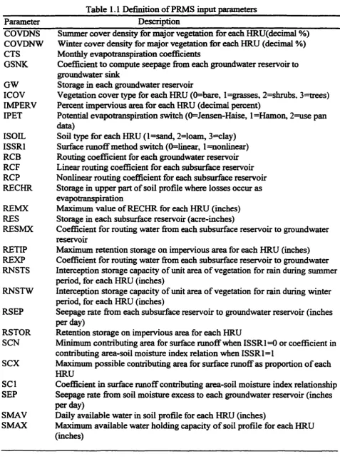
recharge. The input parameters required by PRMS include daily values of minimum and
maximum temperatures, precipitation firom rainfall and snow, as well as solar radiation. In
addition to these, the physical characteristics of each HRU are also defined as input (see
Table 1.1). Daily climatic data can be extrapolated for each HRU using a set of user-defined
adjustment coe£5cients developed from regional climate data. Three procedures are available
to compute potential evapotranspiration (PET) (Leavesley and Stannard, 1990a). These are:
(1) a procedure that uses daily pan-evaporation data and a monthly pan-adjustment
coefiRcient, (2) the Hamon equation (see appendix) which computes PET as a function of
daily mean air temperature and total hours of sunshine and (3) the Jensen-Haise (see
appendix) equation that computes PET using air temperature, solar radiation, elevation, vapor
pressure, and type of vegetation cover. The choice of a procedure is dictated by the
availability of data. In this study daily minimum and maximiim air temperature data were
available, while solar radiation data were incomplete; thus the Hamon equation was used to
compute the PET.
PRMS has undergone various modifications and refinements. The original version of
the model was derived from two previous developed models; the Mountain Watershed
Simulation Model (Leavesley, 1973), and the Distributed Routing Runoff Model (Dawdy et
al., 1978). Since its development in the early 1980s, PRMS has been utilized for various
studies of surface runoff (Parker and Norris, 1989; Fontaine, 1989; Bower, 1985; Gary, 1984;
Carey and Simon, 1985). Leavesley and Striffler (1979) used PRMS to assess the impact of
snowmelt on total runoff. Interest in global climate change has further necessitated the
application of the model to assess the impact of variable rainfall and temperature regimes on
streamflow. Leavesley et al. (1992) used PRMS to assess various scenarios of global change
on surface runoff. PRMS has also been used to study the possible effects of deforestation on
surface runoff in Oregon (Allen and Laenen, 1993; Risley, 1994). Apart from silviculture,
the effects of other agricultural activities on annual streamflow have not been studied by
Table 1.1 Definition of PRMS input parameters
Parameter Description
COVDNS Summer cover density for major vegetation for each HRU(decimal %)
COVDNW Winter cover density for major vegetation for each HRU (decimal %)
CTS Monthly evapotranspiration coefiBcients
GSNK Coefficient to compute seepage from each groundwater reservoir to
groimdwater sink
GW Storage in each groundwater reservoir
ICOV Vegetation cover type for each HRU (0=bare, l=grasses, 2=shrubs, 3=trees)
IMPERV Percent impervious area for each HRU (decimal percent)
IPET Potential evapotranspiration switch (0=Jensen-Haise, l=Hamon, 2=use pan
data)
ISOIL Soil type for each HRU (l=sand, 2=loam, 3=clay)
ISSRl Surface runoff method switch (0=linear, l=nonIinear)
RGB Routing coefficient for each groundwater reservoir
RCF Linear routing coefficient for each subsurface reservoir
RCP Nonlinear routing coefficient for each subsurface reservoir
RECHR Storage in upper part of soil profile where losses occur as
evapotranspiration
REMX Maximum value of RECHR for each HRU (inches)
RES Storage in each subsurface reservoir (acre-inches)
RESMX Coefficient for routing water from each subsurface reservoir to groundwater
reservoir
RETIP Maximum retention storage on impervious area for each HRU (inches)
REXP Coefficient for routing water from each subsurface reservoir to groundwater
RNSTS Interception storage capacity of imit area of vegetation for rain during sxmimer
period, for each HRU (inches)
RNSTW Interception storage capacity of unit area of vegetation for rain during winter
period, for each HRU (inches)
RSEP Seepage rate from each subsurface reservoir to groundwater reservoir (inches
per day)
RSTOR Retention storage on impervious area for each HRU
SCN Minimum contributing area for surface runoff when ISSRl =0 or coefficient in
contributing area-soil moisture index relation when ISSR1=1
sex Maximum possible contributing area for surface runoff as proportion of each
HRU
SCI Coefficient in surface runoff contributing area-soil moisture index relationship
SEP Seepage rate from soil moisture excess to each groundwater reservoir (inches
per day)
SMAV Daily available water in soil profile for each HRU (inches)
SMAX Maximum available water holding capacity of soil profile for each HRU
Several ^>proaches have been suggested that utilize GIS tools in delineating HRUs
for PRMS application. Leavesley and Stannard (1990a, 1990b) presented a polygon-<}IS
approach, ^iiile Battaglin et al. (1993) presented a grid-GIS ^jproach. In the polygon
approach, the watershed is partitioned into polygons, each defined to be a distinct spatial unit
In the grid approach, a set of grid squares is considered to constitute a HRU and a
weighted-average parameter is computed for each HRU. In PRMS, the hydrologic characteristics of
each spatial unit are considered and entered as parameters. Characteristics sometimes
considered are slope, aspect, elevation, vegetation type, soil type and distribution of
precipitation. The partitioning criterion is neither standard nor automatic, but requires the
modeler's intuition in defining the HRUs. The sum response of each HRU, weighted on a
unit area basis, provides the daily system response and streamflow from watershed. Daily
runofif from precipitation on a pervious snow fi^ HRU is computed using a contributing area
concept (Dickinson and Whiteley, 1970).
PRMS is designed to simulate continuous (daily) and storm-event runoff, which are
presented as options where choice is determined by whether precipitation data is available as
breakpoint data (in time steps of several minutes for a storm event) or as daily data step. In
this research the daily precipitation option was used to simulate streamflow for a time period
of one calendar year. The watershed was partitioned into 22 HRUs, for the simulation.
Leavesley (1983) explains that PRMS is designed as a system of modules that
provides the desired flexibility and data management capability for the incorporation of
user-specific requirements. The design and development of the modeling system allow it to: (1)
simulate mean daily flows and shorter time-interval storm-flow hydrographs for any
combination of meteorological and physical characteristics data, (2) provide capabilities for
system enhancement, (3) provide sensitivity analysis capabilities, and (4) provide a
data-management capability that is compatible with the United States Geological Survey's
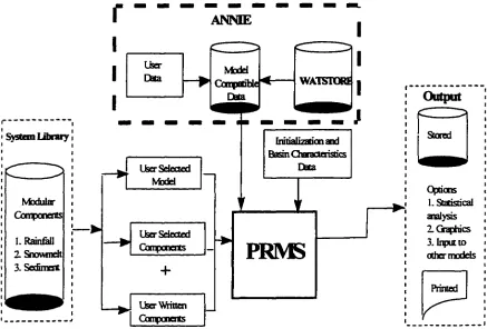
WATSTORE system. The input and output data for PRMS are managed by a USGS
watershed management system ANNIE (Lumb et al. 1990). Figure 1.1 shows the schematic
representation of the PRMS modeling components and the relationship between PRMS and
ANNIE
S>stanLiliraiy
Nfcduiar
Conixments
1. RainM
2. Snowneh
3. Seifinm
VIodel
Cornpoibie
<
WATSTOML^Sdected MkU
User Written Qxnpcnercs Usa Selected Ganpcnens
bihializatiaaand Basin Charactaistics
Dtta
PRIVK
Output
Stored
Options I. Statistical analysis 1 Graphics 3. Input to ether models
[image:17.619.79.516.220.516.2]Printed
Figure 1.1 PRMS System Components,
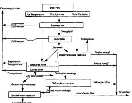
The conceptual watershed system is comprised of a series of reservoirs, whose
outputs are combined to produce the total system response (Figure 1.2). Precipitation inputs
are in the form of rain, snow, or both. Initial precipitation is reduced by interception, and
whatever remains is treated as the net precipitation amount Temperature and solar radiation
are the energy inputs that drive the processes of evaporation, transpiration, sublimation and
snow melt- The reservoirs are the impervious zone, soil zone, subsurface zone, and the
groundwater zone.
Visualization of Hydrological Processes
Visualization of Natural Phenomena
Technological developments in the field of information technology are providing
scientists with powerful tools to analyze, visualize, and display data. Orland (1992) reports
that user expectations of data output have evolved to the point where ease of use and clarity
of interpretation are very critical. The role of visualization in the presentation of model
results helps to convey the impact of alternative man£^ement plans and landuse scenarios.
White et al. (1996) report that developments in computer mapping and analysis have
provided the means to accurately analyze hydrologic data sets, such as streamflow and
precipitation measurements over extended periods of time. White et al. (1996) also reported
an ongoing investigation on different methods of visualizing temporal aspects of floods.
They considered three methods: (1) color-coding of stream networks, (2) iconic
representation of flow by dynamic symbols whose velocity varies with the rate of
streamflow, and (3) variation in the representation of stream channel thickness. They
selected the 1993 United States Midwest floods as the case study for system implementation
and generated a series of maps representing floods. They concluded that maps, though
comprehensible to people who imderstand GIS, needed to be adapted to a form available to
the public. This study developed visualization procedures intended to visualize hydrologic
Evapotranspiration
i i
Evaporation
INPUTS
Air Temperature Precipitation Solar Radiation
Sublimation
Sublimation
Evaporation
Interception
I
Throu^fiillSnowpack
Snawmelt
Evapmtttion
Impervious zone reservoir
Suiface runoff
Transpiration
Transpiration
Recharge Zone Lower Zone
u
zonee.Surface nmff
Ground-wefer recharge
Subsurface recharge
t
-wcfer recharge
T ^
Gnfmd-Subsurface reservoir Subsurface flow
Ground-water reservoir
I
Groundwater Sink
Ground-water recharge
Groundwaterflow Streamflow
[image:19.625.91.551.174.533.2]•
Figure 1.2 Conceptual Watershed System
Visualization and GIS
The visualization procedures embodied in this study reflect one dimension of graphics
discussed by Ganter (1994): exploratory graphics. Exploratory graphics portray the
information generated from numerical simulations or other modeling, especially where there
is a need to simplify the presentation or render it less ambiguous or more convincing. Ganter
(1994) states "These graphics usually mimic the appearance of the object or process being
studied, and are often dynamic, showing behavior over time." This study generates a product
that presents results in a maimer simple and less ambiguous than charts or graphs.
When designing a visualization one must determine what phenomenon needs to be
displayed, and also the form of presentation, so that the defined cognitive tasks can be
achieved. It is necessary to rationally address the relationship between the communication
objectives and the nature of the display within a user-centered, cognitive ergonomics
framework suggested by Turk (1994). A major cognitive task considered in this study was
phenomenon change visualization. This means that the visualization depicts phenomenon
change over some specified time period, with an adjacent legend indicating the rate of change
of a simulated variable with time.
While developing the visualization, there was also a need to develop a system close to
"realism." Such "realism" is defined as bearing resemblance to the visual appearance of the
"physical terrain" (a landscape surface) and "physical entities" (in this case the stream). The
visualization product generated in this study was intended to explain the results of the model
simulations. Bishop and Leahy (1989) contended that as decision-making became
increasingly an exercise in public consultation and compromise, decision-support would
require that all aspects of a project be clearly understood by the public. A visualization
technique that transcends skill, experience, and awareness levels should also reduce the scope
for differences of opinion brought on by differences in interpretation. In enhancing the
"imagery" for decision-makers, there is the ever-prevailing need for "realism." "Realism"
becomes difficult when the visualization developer has to visualize complicated phenomena.
Several criteria have to be satisfied. To attain this goal: (1) the shape of the graphic product
the background (landscape surface) itself and (3) additional attributes should be
'Visualizable."
Scope of Research
This study sought to develop a set of procedures to assist the decision making process
in agricultural watershed management. The research's major components involved: (1)
accurate modeling of the hydrology of an agricultural watershed, (2) enhanced presentation
of simulated hydrology to decision-makers, and (3) the exploration of alternative
management options available. The study focused on the role of streamflow as a major
indicator of a watershed's hydrology.
Study Objectives
The objectives of this study are to:
1. Evaluate the performance of a widely used distributed-parameter model in the simulation
of the surface hydrology of an agricultural watershed.
2. Develop a technique to visualiTe and enhance understanding and presentation of the
modeling results using current management practices.
3. Examine the effectiveness of alternative watershed and management practices through the
use of the simulation model and visualization.
Research Plan
In this research, data from the Four-Mile Creek watershed in east central Iowa, were
used to achieve the three objectives. Studies by Johnson and Baker (1980) generated the data
that were used as inputs to the model and for model calibration and validation. These data
were combined with relevant data from other sources to evaluate the performance of PRMS
in predicting the hydrologic conditions of the watershed. GIS techniques were used to
assemble, organize, and manipulate watershed data for input in the modeling system.
Elevation data for Four-Mile Creek was used to generate a digital terrain model (DTM), and
GIS and animation done by visualization software accessed from the UNIX interface of a
Silicon Graphics Inc. (SGI) platform. Modeling results showing the impacts of alternative
land management changes on surface runoff were visualized using the developed procedures.
Dissertation Organization
This dissertation comprises of three papers, each of which address one of the three
research objectives. The first paper entitled "Implementation of a Precipitation-Runofif
Model in an Agricultural Watershed " is to be submitted to the Journal of Hydrology. The
second paper entitled "Visualization of Simulated Surface Runoff of an Agricultural
Watershed" is to be submitted to the Transactions of the American Society of Agricultural
Engineers (ASAE). The third paper entitled "Impacts of Alternative Land Management
Scenarios on Surface Hydrology " is to be submitted to the Journal of the American Water
Resources Association. All papers have an abstract, introduction, methodology, results and
discussion, conclusions and references. These papers are followed by a general conclusion
for the entire research.
References
Allen, R. L., and Laenen, A. 1993. Preliminary Results of the Simulation of Oregon Coastal Basins Using Precipitation-Runofif Modeling System (PRMS). US Geological Survey,
Investigations Report 92-4108, 99p.
Battaglin, W. A., Hay, L. E. Parker, R. S., and Leavesley, G. H. 1993. Applications of GIS for Modeling the Sensitivity of Water Resources to Alterations in Climate in the
Gunnison River Basin, Colorado. Water Resources Bulletin 25:1021-1028
Belval, D. L., Woodside, M. D., and Campbell, J. P. 1994. Relation of Stream Quality to Streamflow and Estimated Loads of Selected Water-Quality Constituents in the James and Rappahanok Rivers Near the Fall Line of Virginia, July 1998 through June 1990. US
Geological Survey, Water Resources Investigations Report 94-4042, 97p.
Bower, D.E. 1985. Evaluation ofthePrecipitation-RimoffModeling System, Beaver Creek Basin, Kentucky. U.S. Geological Survey, Water Resources Investigations Report
84-4316. I21p.
Brooks, K. N., FfoUiot, P. F., Gregersen, H. M., and Thames, J. L. 1991. Hydrology and the Management of Watersheds. Iowa State University Press, Ames, lA. 456p.
Carey, W. P., and Simon, A. 1984. Physical Basis and Potential Estimation Techniques for Soil erosion Parameters in the Precipitation-Runoff Modeling System (PRMS). U. S.
Geological Survey, Water Resources Investigations Report 84-4218, I26p.
Cary, L. E. 1984. Application of the US Geological Survey Precipitation-Rimoff Modeling System to the Prairie Dog Creek Basin, Southeastern Montana. U. S. Geological Survey,
Water Resources Investigations Report 84-4178, 124p.
Dawdy, D. R., Schaake, J. C., Jr., and Alley, W. M., 1978. Distributed Routing Rainfall-Runoff Model. U.S. Geological Survey Water Resources Investigations Report 78-90,
151p.
Dickinson, W. T. and Whiteley, H. Q. 1970. Watershed Areas Contributing to RimofF.
International Association of Hydrologic Sciences 96:1.12 - 1.28.
Dixon, R. M., and Peterson, A. E. 1971. Water Infiltration: A Channel System Concept. Soil
Sci. Soc. Amer. Proc. 35:968 - 973.
Dunker, J. J., Vail, T. J. and Melching, C. S. 1995. Simulation of Regional Rainfall-Runoff Relations for Watersheds in Lake County, Illinois: U. S. Geological Survey, Water
Resources Investigations Report 95 - 4023, 118p.
Fontaine, R. A. 1989. Application of a Precipitation Modeling System in the Bald Mountain Area, Aroostook County, Maine. U. S. Geological Survey, Water Resources
Investigations Report 87-4221, 84p.
Ganter, J. 1994. Exploratory Graphics in Visualization Software, pp. 71-80. In Heamshaw, A.M., and Unwin, D. (Editors) Visualization in Geographic Information Systems. John Wiley and Sons, New York, NY.
Johnson, H. P., and Baker, J. L. 1978. Field-to-Stream Transport of Agricultural Chemicals and Sediments in an Iowa Watershed, Part 1: Data Base for Model Testing (1976-1978). U.S. Environmental Protection Agency, Athens, GA.
Leavesley, G. H., and Striffler, W. D. 1979. A Mountain Watershed Simulation Model. pp379-386. In Colbeck, S.C., and Ray, M. (Editors) Modeling of Snow Cover Runoff. US Army CRREL, Hanover, NH.
Leavesley, G.H., Lichty, R. W., Troutman, B. M., and Saindon, L. G. 1983. Precipitation-Runoff Modeling System: User's Manual: U.S. Geological Survey Water Resources
Investigations report 83-4238, 207p.
Leavesley, G. H., and Stannard, L. G. 1990a- Application ofRemotely Sensed Data in a Distributed-Parameter Watershed Model. pp47-64. In Kite, G. W. and Wankiwicz (Editors). Proceedings of Workshop on Applications of Remote Sensing in Hydrology.
National Hydrologic Research Center, Environment, Canada.
Leavesley, G. H. and Stannard, L. G. 1990b. A Modular Watershed-Modeling System for Use in Mountainous Regions: Scweizer Ingenievr und Architekt 18:380 - 383.
Leavesley, G. H., Restrepo, P., Stannard, L. G., and Dixon, M. 1992. The Modular Hydrologic Modeling System - MHMS. pp 263-264. In Herrmann R. (Editor)
Conference on Managing Waters Resources During Global Change. American Water Resources Association, Hemdon, VA.
Lumb, A. M., Kittle, J. L., and Flynn, K. M. 1990. Users' Manual for ANNIE - A Computer Program for Interactive Hydrologic Analyses and data Management: U.S. Geological
Stirvey Water Resources Investigations Report 89 - 4080, 236p.
Moore, 1. D., Norton, T. W., and Williams, J. E. 1993. Modeling Environmental Heterogeneity in Forested Landscapes. J. Hydrol. 150:717-747.
Newson, M. 1994. Hydrology and the River Environment. Clarendon Pess, Oxford, UK. SOOp.
Orland, B. 1992. Evaluating Regional Changes on the Basis of Local Expectations: A Visuali22tion Dilemma. Landscape and Urban Planning 21: 257-259.
Parker, R. S. and Norris, J. M. 1989. Simulation of Streamflow in Small Drainage Basins in the South Yampa River, Colorado. U. S. Geological Survey, Water Resources
Investigations Report 88-4071, 104p.
Risiey, J. C. 1994. Use of a Precipitation-Runoff Model for Simulating Effects of Forest Management on Streamflow in 11 Small Drainage Basins, Oregon Coast Range. U. S.
Schwab, G. O., Fangmeier, D. D., Elliot, W. J. and Frevert, R. K. 1992. Soil and Water Conservation Engineering, pp. 78-79.. John Wiley and Sons Inc., New York, NY.
Szollosi-Nj^, A., Kundzewicz, Z. and Cordova-Rodriguez, J. 1987. Surface Water Hydrology, pp156-197. In Kundzewcz, Z. (Editor) Hydrology 2000, International Association of Hydrologic Science, Oxfordshire, UK.
Turk, A. 1994 Cogent GIS Visualizations, pp. 26-33. In Heamshaw, A.M and Unwin, D. (Editors) Visualization in Geographic Information Systems. John Wiley and Sons, New York, NY.
White, W. S., Mizgalewicz, P. J., Maidment, D. R., and Merril, K. R. 1996. GIS Modeling and Visualization of the Water Balance During the 1993 Midwest Floods. In A WRA
Symposium on GIS and Water Resources. American Water Resources Association,
Hemdon, VA.
Woodside, M. D. 1994. Landuse in and Water Quality of the Pea Hill Arm of Lake Gaston Virginia and North Carolina- l9Zi-9Q. U. S. Geological Survey, Water Resources
CHAPTER!
EVALUATION OF PERFORMANCE OF A PRECIPITATION-RUNOFF
MODEL APPLIED TO AN AGRICULTURAL WATERSHED
A pq}er to be submitted to the Journal of Hydrology
F. L. Namwamba, U. S. Tim, C. E. Anderson, and R. S. Kanwar.
ABSTRACT
The performance of a distributed-parameter model, the Precipitation and Rimofif
Modeling System (PRMS), was evaluated for an agricultural watershed in east central Iowa.
Observed hydrologic data from 1978 to 1980, derived from a study by Baker and Johnson
(1980), were used for the purposes of model calibration and validation. Calibration from the
1978 data was accomplished in a three step process; (1) the model was calibrated for a
subwatershed; (2) the parameters were transferred and tested on a different larger subsection
of the watershed; (3) parameters were readjusted, then used again in re-calibrating the first
subwatershed; and (4) after the parameters performed satisfactorily for the two subwatersheds
they were applied to the whole watershed. Even though PRMS predicted total annual
streamflow reasonably, in certain cases the model over-predicted or under-predicted
depending on the time and circumstances at the time of the year. After calibration,
calibration results were compared with data for 1979 and 1980. The model generated outputs
that were statistically evaluated to be in reasonable agreement with observed data.
Throughout the study geographic information systems (GIS) proved to be a useflil tool in
distributed-parameter modeling.
INTRODUCTION
The characterization of water balance during major flooding events is useftil to
scientists, land-use planners, and public agencies who need such information to develop
strategies to cope with future floods (White et al, 1996). Streamflow rates and volumes have
floods, erosion potential, and agricultural non-point source pollution. Whereas increased
erosion and agricultural chemical losses are unintended side effects of the highly productive
agricultural systems, research has demonstrated that management practices can be used to
help control these undesirable effects. These practices have to be effective and technically
feasible, as well as socially and economically acceptable. It is therefore necessary for
decision-makers to improve their understanding of issues related to streamflow, and more so
whenever streamflow relates to agricultural practices.
Several types of mathematical models have been developed to address different water
management problems. These models fail into two primary categories: stochastic and
deterministic.. Stochastic models, on the other hand, utilize statistical methods and the laws
of probability to predict events. Deterministic models are those with specific initial
conditions, boundary conditions, and an output known with certainty. Deterministic models
are of two types: lumped-parameter models and distributed-parameter models.
Lumped-parameter models treat the whole watershed or a big portion of it, as one
spatial unit. Several Iimiped-parameter models have been applied to small agricultural
watersheds. Among these models are the USDAHL74 Model (Holtan et al. 1975) as well as
the SCRAM model (Bailey, 1975; Adams and Kurisu, 1976). The Hydrologic Simulation
Program - FORTRAN (HSPF), is an adaptation of the Stanford Watershed Model (an earlier
version) in FORTRAN and is more versatile and comprehensive (Leytham and Johannson,
1979). Indeed, HSPF has been used to study impacts of agriculture on the Four-Mile Creek
watershed (Donigian et al, 1984). With the advent of geographic information systems (GIS),
it is no longer necessary to rely on lumped-parameter models. Instead, nimierous distributed
parameter models have been used to characterize and simulate watershed processes.
Distributed-parameter modeling involves dividing the watershed into smaller spatial
units with uniform characteristics for each unit. The spatially variable hydrologic processes
are considered at various points in the study area. The total output of the watershed is the net
contribution from each spatial unit Rogers et al. (1987) report that distributed-parameter
models are preferred over lumped models due their more realistic output. Examples of
(AGNPS) described by Young et al. (1987) and the Soil and Water Assessment Tool
(SWAT) described by Arnold et al. (1998). The distributed-parameter model selected for
this study is the Precipitation and Rimofif Modeling System (PRMS) developed by Leavesley
etal. (1983).
The primary objective of this study was to evaluate the performance of the
Precipitation-Runoff Modeling System (PRMS) model in the simulation of the surface
hydrology of an east-central Iowa agricultural watershed. This study describes the process
used to determine the important rainfall-runofif characteristics for the Four-Mile Creek
watershed, and presents the results from the configuration and calibration of PRMS in the
watershed. Specifically the study involved: (1) development of a spatial database for use in
the modeling study, (2) the use of GIS techniques to generate and organize input parameters
for model application, and (3) evaluation of the predictive capabilities of the model through
calibration and validation.
METHODOLOGY
Biophysical Modeling
PRMS is a process-based, distributed parameter rainfall-runoff modeling system
designed to analyze the effects of various combinations of climate, landuse, land cover and
terrain on streamflow, sediment transport, and general basin hydrology (Leavesley et al.,
1983). The model was originally developed to examine surface hydrologic characteristics in
the mountain areas of the westem United States. In subsequent years its use has been
extended to characterize the hydrology of forested watersheds.
PRMS has been used to simulate streamflow from several watersheds. Dinicola
(1990) used PRMS to define regional parameters for the forested areas in Oregon. Allen and
Laenen (1993) used the PRMS to analyze hydrologic cumulative effects for three Oregon
coastal watersheds. Their objectives were to present interim calibrations and verifications of
rainfall-runoff models for three basins in Oregon, evaluate streamflow responses from
changes in model parameters that represented changes in forest resource management and to
Leavesley et al (1983) outline the methodology and components of PRMS. The
model divides the terrain into spatial units whose hydrologic response is assumed to be
uniform across the unit The model then simulates the impacts of various combinations of
climate, landuse and terrain on streamflow. PRMS is a deterministic distributed-parameter
model that simulates water-balance relationships, flow peaks and volimies, soil-water
relationships, sediments and groundwater recharge. Inputs required by the model include
daily values of minimum and maximimi temperatures, daily precipitation from snow and
rainfall, and daily solar radiation.
To apply the model the watershed must be partitioned into homogeneous units on the
basis of slope, aspect, elevation, vegetation type, and soil type. The partitioning criteria are
neither standard nor automated. The user has to define the basis for the selection of the
physical characteristics. The resulting units, referred to as Hydrologic Response Units
(HRUs) have a uniform hydrologic response. Each HRU requires input values for slope,
aspect, elevation, vegetation type, and soil type. Water balance and energy balance are
computed for each HRU. The sirai of responses of all HRUs, weighted on a imit area basis,
produces the daily system response and streamflow from the watershed. For storm
hydrograph simulation the watershed is conceptiialized as a series of interconnected
flow-planes and channel segments. Surface runoff is routed over the flow flow-planes into the channel
segments and channel flow is routed through the watershed channel system.
PRMS predicts annual, monthly and daily siunmaries of: rainfall excess, groundwater
flow, subsurface flow, surface runoff, mean daily discharge, inflow to groundwater reservoir
from HRUs, and inflow to subsurface reservoirs. Simulated results and their summaries are
written to output files, and the data used to generate flow hydrographs and other graphical
data.
Description of Study Area
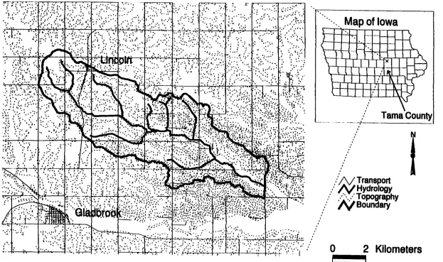
The 50.5km^ Four-Mile Creek watershed is located in the northwestern part of Tama
County in east central Iowa (Figure 2.1). The center of the watershed is located at 42° 12' N
latitude and 92° 35' W longitude. It has a northwest-southeast orientation, with a variable
heavily cropped areas of Iowa, the Four-Mile Creek watershed has a well developed
tile-drainage system. The Four-Mile Creek flows east into the Wolf Creek, which flows east into
the Cedar River. It drains into the Iowa-Cedar River basins m the eastern half of Iowa. Two
approximately parallel rivers, the Iowa and the Cedar, flow to the southeast before
converging and draining to the Mississippi river south of Muscatine, Iowa. Elevation in the
watershed ranges firom about 276 m above sea level in the channel at the outlet, to about
325m above sea level in the upper reaches of the watershed.
With regard to hydrology, Johnson and Baker (1978) supplied the following
information: (1) the average annual runoff per unit area of the watershed from 1962 to 1978
was about 210 mm; while the average discharge was approximately 0.31 mVs, in addition,
flood discharges of about 30 mVs were been reported for the 50.5 km^ area, (2) sediment
yields were about 100 tonnes/km^ but varied across the landscape, (3) drain tiles had been
installed in some fields close to the main channel and in some of the upper regions of the
watershed with less sloping topography and (4) different tillage practices were used for soil
conservation purposes. Primary examples were practices such as conservation tillage,
terraces, and grassed waterways that decrease sediment loss.
Johnson and Baker (1978) further report that the climate of the study area included
cold freezing conditions during the winter months (November to March) and very high
humidity during the summer months (June to September). Temperatures ranged from below
freezing point (0° C) during winter months to more than 32°C during the sununer. Average
aimual rainfall for central Iowa from 1900 to 1978 was 864 mm. High frequency rainfall
events were mainly generated by intense convective storms during the summer and slower
frontal thunderstorm during winter. The Four-Mile Creek watershed was located in Major
Land Resource Area 108 (the Illinois and Iowa Deep Loess Drift) that covers the northeast
portion of the Iowa-Cedar basins. It is characterized by gentle slopes, a smooth relief, and
loamy soils. In more sloping areas of the watershed soil erosion proves to be a major
problem.
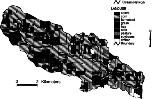
The watershed is heavily cropped with row crops (see Figure 3.2). Johnson and
year 1980. A small percentage of the land along the lower end of the creek and in the steeper
areas of the watershed is under permanent grass and woodland. Johnson and Baker (1980)
report that between 1970 and 1980, the percentage of the watershed in row-crops increased
from 55% to 80%; while land in pasture, hay, grass, oats, government set aside (CRP) and
woodland was reduced.
Data Preparation
Input data for model simulation were obtained from five main sources; (1) existing
data collected by Johnson and Baker (1978), (2) meteorological data from the ISU
Department of Agronomy, (3) existing digital maps from the ISU GIS Support and Research
Facility, (4) manual digitizing of cartographic information from the United States Geological
Survey (USGS) topographic maps, and (5) manual digitizing of data extracted from field
notes and oblique aerial photographs from the EPA study.
Most data extracted from existing records were meteorological and streamflow data.
For the EPA study, a network of rainfall and streamflow gages was established in the
watershed. Data from these gages were collected on a daily basis. The five daily-recording
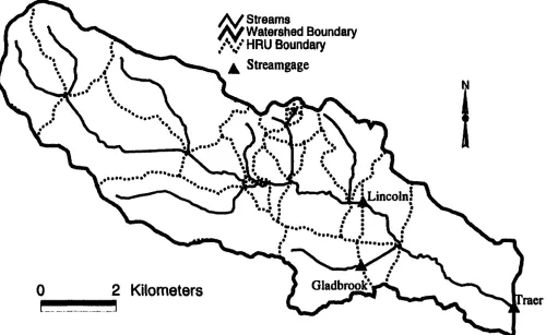
rainfall gages were spatially distributed throughout the watershed (Figure 2.3). The stream
network as well as monitoring and gaging sites used in the study are shown in Figure 2.4.
Streamflow gages were the stage-height recorder type installation. Two of the USGS
streamflow gages were located on a highway and designated as Gladbrook and Lincoln
stream-gage stations. One major streamflow gage was located at the watershed outlet,
designated as the Traer Gage.
Even thoi^ streamflow data were available throughout the year, meteorological data
for the winter months were not collected in the study by Johnson and Baker (1980). To fill in
the gaps for the winter months, meteorological data were estimated by averaging data for two
neighboring weather stations, located at Marshalltown and Traer cities. The watershed is
straddled between the two weather stations. However it should be noted that this data is only
an approximation in lieu of the actual figures.
Existing digital maps were used extensively to provide spatially distributed input
network maps as well as public land survey maps were used to establish reference points for
the background m^ derived from the Tama County database available at the ISU GIS
Support and Research Facility. These reference points were useful when digitizing landuse
map. In Iowa, most roads intersect at the same intersection points as public land survey lines,
which cross perpendicularly at one mile intervals. In addition to these reference points, the
stream network map was derived from a digital hydrography map of Tama County. Soil
maps were obtained from the USDA Digital Soil Laboratory located in the ISU Agronomy
department.
ARC/INFO GIS (ESRI, 1996) was chosen to handle the storage, retrieval,
manipulation, and analysis of spatial data for the watershed. The digital data were acquired
as ARC/INFO export files. Each file is comprised of a public land survey section. After the
files were imported into ARC/INFO, they were built to a correct topology using ARC/INFO
procedures, and then joined into a set of juxtaposed maps using the MAPJOIN command in
ARC/INFO. After being joined the set was subjected to a cleaning process to eliminate sliver
polygons. This process used the ARC/INFO DISSOLVE command and consolidated them
into a single map.
Even though printed maps of the watershed boundary existed from an earlier report
by Johnson and Baker (1980), the maps were not spatially referenced. It was therefore
necessary to manually digitize the watershed boundary from the USGS 7.5 mi^te
topographic maps. Digitizing was accomplished by using a GTCO Super LIIdigitizing tablet
at the ISU GIS Support and Research Facility, with the intersection points from the public
land survey (PLS) lines utilized as digitizing reference points (tic marks). After the boundary
layer was digitized, a contour map layer representing topography was also digitized. Using a
similar approach digital land cover maps were obtained from aerial photographs of the
watershed.
The input and output data for PRMS were managed using the USGS watershed
management system ANNIE (Lumb et al., 1990). ANNIE stores hydrologic data in a
direct-access, binary data library called a Watershed Data Management (WDM) file. ANNIE,
data input facilities from USGS, the input process of ANNIE requires a "one-by-one"
prompting for interactive data entry of each value, a process that would be time consuming
for 30 data sets of365 daUy events representing two calendar years (1978 and 1979). To
eliminate this time consuming step, a method to input data from spreadsheets was devised in
the study. This method followed these procedures: (1) a binary WDM file was exported to a
text format (ASCII), (2) the file headers of the export file were then modified to coincide
with parameters for the Four-Mile Creek input data, (3) the export file was imported into an
EXCEL 5.0 spreadsheet, (4) original data were deleted, and the Four-Mile Creek input data
were typed in the columns to replace the original data, (5) the EXCEL file was exported to
text format, and imported into ANNIE as a WDM import file, and (6) this imported file was
used as the WDM file for Four-Mile Creek watershed.
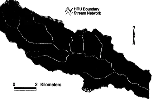
HRUs were defined to be the sub-watersheds ranging from a downstream junction to
upstream, either to the beginning of the stream or to the next junction (Figure 2.5). The
extents of the HRUs were matched with the stream junctions. In the Four-Mile Creek stream
network, 22 stream segments were thus identified. HRUs were defined to be the
subwatersheds for each stream segment. Once allocated, the weighted-average of the areal
proportion of physical characteristics in each subwatershed were computed. In the cases
where nimierical values were required, the weighted-average value was considered to be
uniform over the HRU. In cases where the characteristic required was qualitative in nature,
the dominant (> 50%) characteristic was used as the representative parameter. The only
exceptions to this HRU delineation were in two cases where streamgs^es were located within
the watershed, and were consequently regarded as stream junctions for the purposes of
delineating the HRU. Flow from each HRU empties into only one channel element (outlet),
but each HRU channel inlet can accept multiple subcatchment inflows.
Parameter files were prepared from a simimary of physical characteristics derived
from the digital maps by using GIS techniques. For soil characteristics, landuse and land
management practices this was accomplished by specific procediues performed by the
ARC/INFO GIS. Most of this was done by weighted-averages of polygon features by the
supplied, and ARC/INFO prompted for a characteristic. Thus, soil texture, permeability, and
average slope were thus specified for each HRU. Results fix>m the statistical operation were
then entered into the parameter file, specific to each HRU. Other factors derived from
GIS-techniques were channel lengths and channel slopes.
Parameters for each HRU were specified to compute runoff resulting from rainfall.
Actual measxirement of parameters representing subsurface processes was not practicable.
Therefore reasonable estimate had to be supplied. In most circtmistances, reasonable
estimates of model parameters were obtained from published literature. Parameters to which
the model was most sensitive to are mentioned in the section describing the calibration
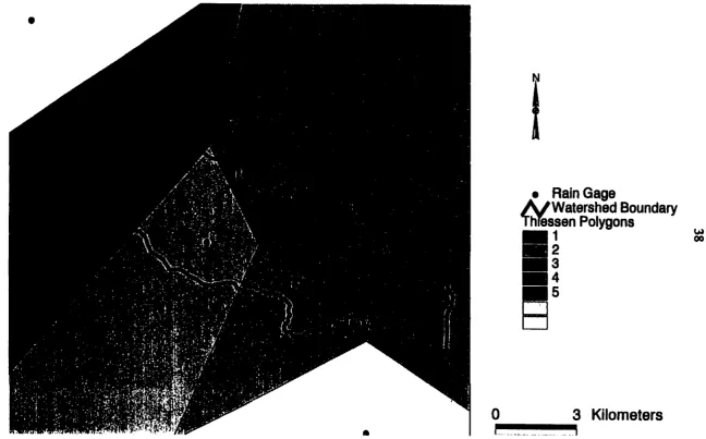
process. Rain gages were allocated to different HRUs using Thiessen polygoning. The
Thiessen polygons were created by the command THIESSEN in ARC/INFO, and the results
are shown in Figure 2.6. After the first run a quick sensitivity analysis was carried out.
Based on the results of this rudiment sensitivity analysis, parameters were then adjusted later
during calibration. Troutman (1985) emphasizes the need for parameters to be physically
realistic and their values to be selected so as to make the simulated peaks and voltmies to
agree well with the observed peaks and volumes.
RESULTS AND DISCUSSION
Calibration of the Model
Observed data were used for calibration and characterization of runoff processes in
the study area. In the process of calibration, sensitivity analyses were used to determine
which parameters the streamflow was most sensitive to. After several such analyses,
tentative simulation model parameters were estimated for calibration of the model. The
ultimate goal of a successfiil calibration process would be to minimiTe the differences
between the observed runoff and the simulated runoff (Thompson, 1989). In the modeling
process judgment was used to select the runoff events to calibrate the model without biasing
the results. Even though workstation PRMS has an internal optimization routine the PC
after the iterative procedure was used. Calibration was conducted on the basis of matching
average daily flow rate.
PRMS was calibrated first for HRU 3, whose outlet is at Gladbrook streamgage
(Figure 2.4), by using observed data for 1978. Initial calibration parameters were adapted
from Cane Branch watershed, ^^ch is located in the Cumberland Plateau physiographic
section of southeastern Kentucky, and were used to help pick the starting model parameters.
The watershed is described by Musser (1963), and is used as a test watershed by the model
developers. As a limited test, parameters were directly transferred and used for initial
simulations. During this test the model over-predicted streamflow by a very high magnitude.
Different values of evapotranspiration parameters were then tried until reasonable
results were obtained. In the early tries, the starting streamflow for the first few days of the
calendar year were too high. These were reduced to reasonable range by the adjustment of
several parameters. The most sensitive parameters were those representing: (1)
air-temperature evapotranspiration coefficient (CTS), (2) vegetation cover density (COVDNS for
summer, and COVDNW for winter), (3) maximum contributing area (SCX), (4) a coefficient
in contributing-area moisture-index relationship (SCI), (5) rain interception storage capacity
in inches (RNSTS for summer and RNSTW for winter), and (6) maximum available water
holding capacity of soil profile (SMAX).
After a reasonable calibration of HRU 3, the parameters were then transferred and
used to calibrate a different larger subsection of the watershed whose outlet was Lincoln
streamgage. There were 18 HRUs upstream firom this streamgage, not including HRU 3.
When the parameters fi-om the initial calibration of HRU 3 were used for simulation, there
was a slight imderestimation of streamflow. A calibration process followed until reasonable
values were obtained.
Once the parameters for a reasonable calibration of Lincoln gage were obtained, the
results were then applied to the whole watershed. Results for the Four-Mile Creek watershed
outlet at Traer streamge^e matched well with those from the Lincoln streamgage.
Streamflows for each month, in cubic-meters per second were averaged and then compared.
of the average monthly observed runoff. When the monthly data were divided in quarters of
"January-March", "April-June", "July-September", and "October-December", the
predicted/observed ratios of mean runoffs were 91%, 107%, 99% and 81% respectively. The
parameters were adjusted within their defined ranges. At the final stage any attempts to
adjust the parameters to obtain a perfect match would push the parameter values beyond the
recommended (reasonable) ranges.
The model has problems simulating late March snowmelt This problem probably
arises because the groundwater seepage parameter RSEP is set uniform for the whole year for
the watershed. When the season proceeds jBx>m winter to spring the model does not
incorporate changes in subsurface thawing conditions. Hence when the first rainfall occurs in
April the movement of water through soil is slower, and the observed values are higher than
predicted. The configuration of the model makes two assimiptions that affect the accuracy of
simulation under agricultural conditions in the US Midwest: 1) that vegetation cover density
is uniform throughout siunmer, and 2) that transpiration conditions are uniform throughout a
month. Hence, in June it is assimied that there is a similar vegetation canopy as May. In
reality the row-crops (particularly com) grow to full canopy in Jxme and hence intercept more
rainfall and there is an over-prediction. This effect is leveled out in July when the water
requirements of the crops are at highest levels and more water is lost through more
transpiration in the later part of the month. The model generally under-predicts streamflow
in the quarters related to winter. It is plausible that soil parameters set uniformly for the
whole year are responsible for this observation.
Tile flow, a imique characteristic of agricultural watersheds in Iowa, is not accounted
for in PRMS. Johnson and Baker (1978) report that many stream valleys have drainage tiles,
designed to drain the topsoil in 24 hours. Once water enters the tiles it flows fi^eely rather
than infiltrate. Drainage flow would to have be modeled by a specific model like
DRAINMOD. (Schwab, 1994). The fact that tile flow was not accounted for constitues a
possible impediment to accurate forecasting of streamflow.
When the streamflows firom Gladbrook, Lincoln and Traer streamgages were
Gladbrook and Lincoln streamgages do not sum up to equal the flow at Traer streamgage.
There seem to be subsurface characteristics at the stream-bed that cause the disappearance of
flow below the surface. Two possible reasons can be inferred to as being responsible for this
behavior: (1) the tributary or the stream as a whole could be a losing stream. Meaning that as
the stream progresses on downstream, it loses water to the subsurface, and (2) there may be a
high component of subsurface flow in the watershed. Since the stream gage accoimts only
for flow above the surface, the unexplained flow anomalies could be attributed to phenomena
below the surface.
Validation of Model
After the model calibration was complete, evaluation was carried out for the years
1979 and 1980. Table 2.2 shows statistics of average monthly streamflows. Several
performance meastires were considered to assess the validation. These were: maximum error
(ME), percent root mean square error (RMSE), Nash-Sutcliffe (NSR), modeling efficiency
(EF), and coefficient of residual mass (CRM). The mathematical expressions for these
performance measures (Loague and Green, 1983) are as follows:
ME = max [x/ - y i \ / = a t o n )
RMSE = 100
1 / 2
>-I
n
Z o . - y ) ' NSR=-^
EF = — /»1
[ ty> - I - . ]
CRM = —^ :=!
n
I.y-M
Where n is the number of pairs of observed (y^ and model simulated (x^) values, and
y is the mean value of the observations. Loague and Green (1983) explain that for the
model to be considered valid (and representative of the real physical system), the hope of the
modeler is to have values of ME, RMSE, NSR, EF and CRM eqiial to 0.0,0.0, 1.0, 1.0 and
0.0 respectively. Both EF and CRM can be negative, and the NSR represents the measure of
the proportion of the total variance of observed data explained by the simulated results.
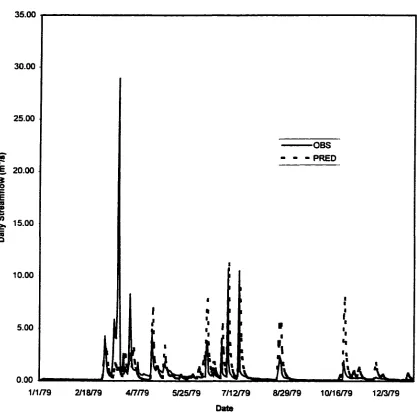
From the results of validation of the year 1979 the values for the performance
measures were as follows: ME = 1.98 mVs, RMSE = 105.92, NSR = 1.61, EF = 0.25, and
CRM = -0.17. For the year 1980 the values for the performance measures were ME = 0.50,
RMSE = 69.93, NSR = 0.50, EF = 0.34, and CRM = -0.25.
For both years the model generally over-predicted the observed total volume of flow,
particularly for the month of November. For 1979 the monthly average and total streamflows
were highly over-predicted because of an anomaly in the month of March, when a peak of
100 cfs was observed. The high discrepancy between this peak and the predicted value
suggests an instrument malilmction. It is this value that makes the Nash-Sutcliffe R* value to
be higher than 1.0. When the months were divided into quarters, it was observed that
validation conditions generally under-predicted streamflow in the first half of the year, and
over-predicted in the last half. When field conditions and parameter definition in PRMS are
examined, and statistical values considered the validation were not unreasonable. Several
factors come into question as an explanation to this discrepancy.
The years 1979 and 1980 were generally wetter than the year 1978. In the model
validation, monthly evaporation parameters (CTS) from the calibration done with the 1978
data were transferred for 1979 and 1980 simulations. However, with more rainfall and a
cooler year (from temperature values), evaporation conditions for 1979/80 were not identical
to 1978. It should also be noted that the year 1979 has one very high value for streamflow,