Ecosystem responses to elevated CO2 using airborne remote sensing at Mammoth Mountain, California

https://doi.org/10.5194/bg-15-7403-2018 © Author(s) 2018. This work is distributed under the Creative Commons Attribution 4.0 License.

Ecosystem responses to elevated CO

2

using airborne remote

sensing at Mammoth Mountain, California

Kerry Cawse-Nicholson1, Joshua B. Fisher1, Caroline A. Famiglietti1, Amy Braverman1, Florian M. Schwandner1,2, Jennifer L. Lewicki3, Philip A. Townsend4, David S. Schimel1, Ryan Pavlick1, Kathryn J. Bormann1, Antonio Ferraz1, Emily L. Kang5, Pulong Ma5, Robert R. Bogue1, Thomas Youmans1, and David C. Pieri1

1_{Jet Propulsion Laboratory, California Institute of Technology, Pasadena, CA, USA}

2_{Joint Institute for Regional Earth System Science and Engineering, University of California Los Angeles,}

Los Angeles, CA, USA

3_{United States Geological Survey, Menlo Park, CA, USA} 4_{University of Wisconsin-Madison, Madison, WI, USA} 5_{University of Cincinnati, Cincinnati, OH, USA}

Correspondence:Kerry Cawse-Nicholson ([email protected]) Received: 6 February 2018 – Discussion started: 3 April 2018

Revised: 17 October 2018 – Accepted: 2 November 2018 – Published: 14 December 2018

Abstract. We present an exploratory study examining the use of airborne remote-sensing observations to detect eco-logical responses to elevated CO2emissions from active

vol-canic systems. To evaluate these ecosystem responses, exist-ing spectroscopic, thermal, and lidar data acquired over for-est ecosystems on Mammoth Mountain volcano, California, were exploited, along with in situ measurements of persis-tent volcanic soil CO2fluxes. The elevated CO2response was

used to statistically model ecosystem structure, composition, and function, evaluated via data products including biomass, plant foliar traits and vegetation indices, and evapotranspira-tion (ET). Using regression ensemble models, we found that soil CO2flux was a significant predictor for ecological

vari-ables, including canopy greenness (normalized vegetation difference index, NDVI), canopy nitrogen, ET, and biomass. With increasing CO2, we found a decrease in ET and an

increase in canopy nitrogen, both consistent with theory, suggesting more water- and nutrient-use-efficient canopies. However, we also observed a decrease in NDVI with increas-ing CO2 (a mean NDVI of 0.27 at 200 g m−2d−1 CO2

re-duced to a mean NDVI of 0.10 at 800 g m−2d−1CO2). This

is inconsistent with theory though consistent with increased efficiency of fewer leaves. We found a decrease in above-ground biomass with increasing CO2, also inconsistent with

theory, but we did also find a decrease in biomass vari-ance, pointing to a long-term homogenization of structure

with elevated CO2. Additionally, the relationships between

ecological variables changed with elevated CO2,

suggest-ing a shift in couplsuggest-ing/decouplsuggest-ing among ecosystem struc-ture, composition, and function synergies. For example, ET and biomass were significantly correlated for areas without elevated CO2 flux but decoupled with elevated CO2 flux.

This study demonstrates that (a) volcanic systems show great potential as a means to study the properties of ecosystems and their responses to elevated CO2emissions and (b) these

ecosystem responses are measurable using a suite of airborne remotely sensed data.

Copyright statement. The author’s copyright for this publication is transferred to California Institute of Technology.

1 Introduction

di-rect effects of carbon dioxide on plant growth (Norby et al., 2016). The last, which proposes that increased atmospheric CO2yields increased photosynthetic rates, is both the most

probable and the most controversial. Although a multitude of experiments have shown positive photosynthetic responses to increased CO2 consistent with the observed growth in the

terrestrial sink (Drake et al., 1997), many ecologists have argued that plant growth in intact ecosystems is limited by water, light, or nutrients rather than CO2 (Körner, 2006;

McGuire et al., 1995).

The Free-Air Carbon dioxide Enrichment (FACE) exper-iments, introduced in the 1990s, allow for CO2fertilization

of intact ecosystems by creating controlled fumigation con-ditions without the use of a growth chamber (Lewin et al., 1994). The FACE studies have been invaluable to our under-standing of the CO2effect, which contributes to the largest

uncertainties in projections of Earth’s climate. These stud-ies have shown some consistent responses indicative of en-hanced growth (Norby et al., 2016), as well as other phys-iological, morphological, and ecosystem consequences, but also suffer from several structural limitations. Perhaps most notably, only short-term study periods are feasible, and it is difficult to measure slower processes like plant acclimation, shifts in species dominance induced by CO2, or other

long-term mechanisms mediated by changes to soil organic matter and nutrients. This is where the long-term localized emis-sions of volcanic CO2can play a game-changing role in how

to assess the long-term CO2effect on ecosystems.

As a result of limited empirical evidence for the strength of CO2fertilization effects, global carbon cycle models

dis-agree about the significance of their associated impacts. Some models show very large CO2effects, while others

indi-cate a smaller or saturating effect (Kolby Smith et al., 2015). Because future predicted fossil carbon uptake is highly de-pendent on the strength of the simulated CO2fertilization,

any constraints on the long-term effect of elevated CO2 on

ecosystems would be valuable in reducing uncertainty in coupled carbon–climate models (Friedlingstein et al., 2014). Persistent diffuse volcanic CO2emissions through soils

re-sult from the degassing of magma beneath volcanoes and of-fer a continuous natural experiment to study vegetation re-sponses to elevated CO2that is expansive in both space and

time. These surface discharges yield broad atmospheric en-hancements that transport CO2 downwind (Kerrick, 2001),

resulting in swaths of variably affected plants whose peri-ods of exposure can be over hundreds of years (Cook et al., 2001). Because volcanic CO2 emissions are a vital part of

the global carbon cycle (Mason et al., 2017; Schwandner et al., 2017) and have been monitored worldwide for decades (Boudoire et al., 2017; Camarda et al., 2012; Perez et al., 2011; Gerlach, 1991), the rate and spatial distribution of these fluxes are well-understood due to an abundance of field surveys in many volcanic systems (e.g. Lewicki et al., 2014; Giammanco et al., 2007; Cardellini et al., 2003; Werner and Brantley, 2003; Hernández et al., 1998). The “kill zone” is

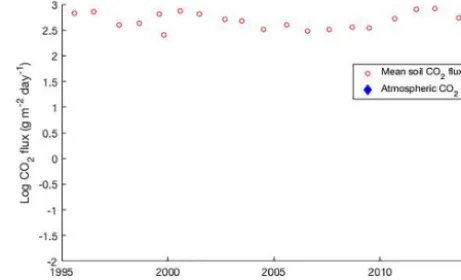
Figure 1.The USGS has measured elevated soil CO2flux at Horse-shoe Lake for the past 2 decades (Werner et al., 2014). These val-ues are consistently higher than the atmospheric CO2measured by USGS California Volcano Observatory eddy covariance station at Horseshoe Lake at the time of the AVIRIS overpass on 21 October 2014.

the exact location where CO2is emitted through the soil – a

property of the soil being altered by the emission. Although the spatial distributions of CO2emissions within tree-kill

ar-eas have been well mapped (List et al., 2005; Werner and Brantley, 2003; Pickles et al., 2001, and others), linking CO2

measurements to vegetation responses along a spatially dif-fuse CO2degassing continuum (outside of the tree-kill zone)

is a natural yet underutilized opportunity for studying the ef-fects of elevated CO2 on plants (Schwandner et al., 2004).

Furthermore, many CO2emissions in volcanic systems have

been ongoing for decades or centuries, thus allowing for the observation of equilibrium, long-term ecosystem responses after transient and acclimational responses have passed.

While FACE experiments may demonstrate ecological re-sponses to increased CO2 at the outset of elevation, studies

in volcanic areas can do the same on super-century scales. However, because volcanic emissions can affect entire land-scapes differentially depending on the flow dynamics of the gas, they require new and innovative techniques for analy-sis. Remote-sensing observations allow for detailed measure-ments across a wide spatial extent that can be used to analyse ecological indicators of CO2effects.

Here, we present an exploratory study examining the use of airborne remote-sensing data to detect ecological re-sponses to elevated volcanic CO2 emissions. It is a

funda-mental principal of volcanology that all active volcanoes emit CO2continuously during their entire life cycle. We leveraged

existing data over Mammoth Mountain, California – a much-studied volcano that has been passively emitting CO2at high

concentrations through faults and fissures on its flanks. The emissions have been measured systematically since a large earthquake swarm in 1989, and their variability has been well documented by repeated CO2 efflux mapping (Lewicki et

1 shows that the elevated soil CO2 fluxes, measured by the

USGS over a span of 2 decades, far exceed the atmospheric CO2measured by a flux tower at the same site.

We developed a statistical framework for examining the relationships between field measurements of soil CO2

emis-sions into the air below the forest canopy and a suite of re-motely sensed ecological variables. In this investigation, we aim to (i) evaluate the viability of using a passively degassing volcanic system to study the properties of ecosystems, (ii) as-sess the detectability of ecological responses to elevated soil CO2emissions via airborne data alone, and (iii) present key

lessons enabling future studies to extend our framework to other biomes. This methodology can be applied to any site that is exposed to elevated CO2.

2 Methods

2.1 Data

Airborne remote-sensing data from multiple sources have been acquired over Mammoth Mountain, California, USA, providing a substantial means to assess ecosystem struc-ture (products derived from lidar, such as canopy height and biomass), composition (products derived from spectral data, such as vegetation indices and plant foliar traits), and func-tion (data products derived from thermal data, such as evap-otranspiration). Figure 2 illustrates several of the different products used in this study, highlighting the diversity of data sources and spatial resolutions.

Mammoth Mountain is an upper montane forest ecosys-tem, characterized by abundant Pinus contorta (lodgepole pine) and also by mature stands of Abies magnifica (red fir),Pinus jeffreyi(Jeffrey pine),Pinus albicaulis(whitebark pine), and Juniperus occidentalis (western juniper) (Potter, 1998). The elevation of our study areas ranged from 2700 to 2950 m. Tree-kill soils are immature High Sierra soils formed from granite, pumice, rhyolite, and obsidian parent materials (McGee and Gerlach, 1998).

2.1.1 Ground measurements

We investigated soil CO2 fluxes within five actively

de-gassing areas on Mammoth Mountain documented by Werner et al. (2014) in 2011 and 2012, which represents a period of relatively high emissions (up to 2000 g m−2d−1of CO2). As described by Werner et al. (2014), fluxes were

mea-sured along fixed grid points using the accumulation cham-ber method (Rahn et al., 1996). In situ measurements were obtained using a West Systems® (Florence, Italy) portable flux meter equipped with a LI-COR820 infrared gas anal-yser. Based on statistical analysis, Werner et al. (2014) found soil CO2fluxes measured within areas of volcanic CO2

emis-sions to be significantly elevated over background areas that were dominated by soil respiration of CO2. Maps of soil

CO2 flux were simulated from in situ measurements at 1 m

resolution using a sequential Gaussian simulation algorithm by these authors, and we resampled their data to the Air-borne Visible/Infrared Imaging Spectrometer (AVIRIS) res-olution (13 m) using nearest neighbour resampling. Conven-tionally, studies of diffuse soil degassing of CO2 on

volca-noes have emphasized an understanding of the modes, loca-tions, geometries, and changes in volcanic flank degassing for purposes of volcanological research, hazard assessment, and monitoring. In many cases, volcanologists have focused on areas associated with sufficient emissions of heat and CO2

for vegetation to have been killed off. In this study how-ever, we focused on vegetated areas where somewhat more mildly enhanced levels of volcanic CO2emissions into the

forest ecosystems might be beneficial for plant growth rather than the reverse. As such, we investigated zones and gradi-ents around tree-kill areas, excluding areas that were barren or contained dead trees by filtering by fractional vegetation cover, where appropriate. The tree-kill areas have local soil conditions that are not representative of the larger ecosys-tem. In addition, because tree-kill areas on Mammoth Moun-tain are largely associated with “cold” CO2 emissions, we

completely avoided confounding influences of hydrothermal heat or acidic vapour emission on ecosystem response. In-deed, there is no significant H2S nor any SO2present at soil

levels at this site, and CO2makes up∼99 % of the gas by

volume; see, for example, data in Werner et al. (2014) and Sorey et al. (1998), and a number of papers on volcanic de-gassing at Mammoth Mountain (Lewicki 2014, 2012, 2008, 2007, 2006). The remaining 1 % is made up of N2and O2.

The use of a high spatial-resolution time-averaged (to limit the influence of varying meteorological conditions) map of canopy-level atmospheric CO2concentration would

be most applicable to assess ecosystem response to elevated atmospheric CO2 concentrations. However, such maps are

unavailable. We therefore took advantage of the extensive record of soil CO2fluxes available for Mammoth Mountain.

Although the effects of elevated CO2in the soil may be

dif-ficult to de-convolve from elevated CO2in the atmosphere,

we treat their effects uniformly. Implications of this are dis-cussed below.

Although the airborne datasets cover a wider region, only points with associated soil CO2 flux measurements were

used to derive our models. The CO2 flux measurements

were spatially resampled to match the resolution of the other datasets, which resulted in small estimations with low confi-dence along the edges. To avoid spurious model fits, edge points with CO2<5 g m−2d−1 were excluded, where the

CO2range is [0,2000] g m−2d−1. In the remainder of this

pa-per, analysed points with elevated CO2flux will be referred

to aseCO2.

2.1.2 AVIRIS

im-In situ west systems fluxmeter 1 m resolution

0 CO flux (g m day )₂ -2 -1 2000

ASO lidar 30 m resolution

0 Biomass (Mg ha-1₎ 200

MASTER Thermal Imager

50 m resolution

0 Transpiration (W m-2₎ 120

AVIRIS-C spectrometer

13 m resolution

0 NDVI (unitless) 1

Figure 2.A wealth of remotely sensed imagery has been acquired over Mammoth Mountain. Some data products used in this study include

(a)maps of soil CO₂flux simulated based on accumulation chamber measurements, shown overlaid on aerial RGB image,(b)above-ground biomass derived from the Airborne Snow Observatory (ASO) lidar,(c)evapotranspiration derived from the MODIS/ASTER (MASTER) airborne simulator, and(d)normalized difference vegetation index (NDVI) derived from the Airborne Visible/Infrared Imaging Spectrometer (AVIRIS image).

agery was acquired over Mammoth in October 2014; this flight was chosen from a number of possible surveys of the area to minimize snow cover and also because of its tempo-ral proximity to the eCO2ground measurements. The

stan-dard level 2 (L2) atmospherically corrected reflectance data (Thompson et al., 2015) were used (available from https: //aviris.jpl.nasa.gov/, last access: 19 November 2018), and the data had a spatial resolution of 13 m. These data were collected as part of the NASA HyspIRI Preparatory Airborne Campaign.

Vegetation indices

Vegetation indices are commonly used as an indicator of veg-etation health and/or greenness. While many vegveg-etation in-dices are related, they differ enough to be considered inde-pendent variables. For instance, some account for soil mois-ture, and others weight plant greenness more heavily. This was an exploratory effort in investigating the effects of CO2

on any measure of plant function, composition, and struc-ture, and so we attempted to cover all avenues of investiga-tion. The following indices were derived from the AVIRIS spectral data:

– the normalized difference vegetation index (NDVI) – simple ratio index

– enhanced vegetation index

– red edge normalized difference vegetation index

– modified red edge simple ratio index

– modified red edge normalized difference vegetation in-dex

– Vogelmann red edge index 1.

Each uses a ratio between narrow bands to represent vegeta-tion health as a single index, and all are described more fully in Thenkabail et al. (2016).

Foliar traits

The chemical composition of plants affects light interactions, especially in the short-wave infrared (Singh et al., 2015). Therefore, imaging spectroscopy can be used to map key vegetation properties, especially those affecting carbon and nutrient interactions. Spectral features, derived from data such as AVIRIS, have been shown to correlate significantly with certain chemicals and plant properties, such as carbon, nitrogen, nitrogen isotope 15, leaf mass per area (LMA), cellulose, and acid-digestible lignin (Singh et al., 2015). These properties are associated with photosynthesis, light-harvesting ability, and nutrient fluxes and can be used to characterize vegetation responses to disturbances or climate trends (Townsend et al., 2008).

uncertain-ties, were used to derive partial least squares regression mod-els for each trait. Since these equations were derived in the nearby area of the Sierra Nevada, these equations were ap-plied to the BRDF-corrected AVIRIS data used in this study. Infeasible negative numbers were removed for the mod-elling.

2.1.3 MASTER

The MODIS/ASTER (MASTER) airborne simulator ac-quires data in 50 channels between 0.4 and 13 µm. We uti-lized the five thermal channels (10–13 µm), which had been processed to Level 2 (available from https://master.jpl.nasa. gov/, last access: 19 November 2018). MASTER data were acquired in November 2013, with a 50 m spatial resolution. Land surface temperature

The five thermal bands from MASTER were used to calcu-late land surface temperature (LST) in a standard Level 2 product. The acquired data were processed to radiance using MODTRAN 5.2 for the atmospheric correction, along with a water vapour scaling method (Tonooka, 2005). The tempera-ture emissivity separation (TES) algorithm was then used to derive LST and spectral emissivity (Gillespie et al., 1998).

The MASTER data are at coarser spatial resolution (50 m) compared to the other datasets (e.g. the working resolution for reprojection is the AVIRIS resolution of 13 m). An ideal dataset would have MASTER acquired at 13 m or similar (∼10 m; i.e. the scale of an individual tree canopy), but in order to build a comparable dataset for this analysis, we used two resampling methods: the standard nearest neigh-bour resampling and a statistically principled method pro-posed in Ma et al. (2018). The statistical model propro-posed by Ma et al. (2018) represented LST as a combination of low-dimensional random effects linked with basis functions and a Gaussian graphical model (also called Gaussian Markov random field). As demonstrated by Ma et al. (2018), this model provides a flexible and computationally efficient way to characterize potentially complex and non-stationary spa-tial variability. The parameters of the underlying statistical model were fitted to MASTER LST and evapotranspiration (ET) data at 50 m resolution, using maximum likelihood es-timation via an expectation-maximization (EM) algorithm. The resampled data at 13 m spatial resolution were then gen-erated via conditional statistical simulation in which we re-quired that when aggregated back to the original coarse res-olution, the resampled data matched the original MASTER data exactly.

Evapotranspiration

ET is the key water variable in ecosystem functioning, in-dicating plant water use and loss (Fisher et al., 2017). In this study, ET was calculated using the Priestley–Taylor model used by the Jet Propulsion Laboratory (PT-JPL)

re-trieval (Fisher et al., 2008), which partitions ET into canopy transpiration, soil evaporation, and interception evapora-tion by transforming potential ET (Priestley and Taylor, 1972) into actual ET using ecophysiological constraints. The ECOSTRESS ET retrieval system was used to incorporate MASTER LST as the thermal input (Fisher et al., 2015); ad-ditional ancillary data were incorporated from MODIS and Landsat to constrain meteorological and phenological con-trols on ET (Famiglietti et al., 2018; Verma et al., 2016; Ryu et al., 2011; Kobayashi et al., 2008). The final ET product used here was only the canopy transpiration component (re-ferred to as ET throughout), as our analytical interest lies only in the vegetation response toeCO2.

2.1.4 ASO

The Airborne Snow Observatory (ASO, http://aso.jpl.nasa. gov, last access: 19 November 2018) is a coupled lidar (Riegl Q1560) and spectrometer (CASI-1500) mounted on a King Air A90 aircraft and was originally developed to mon-itor snow in the mountains for water resource management (Painter et al., 2016). The Riegl Q1560 is a dual-scanning li-dar with two 1064 nm laser sources; each scanner is tilted in the along-track direction by±8◦and the cross-track direc-tion by±14◦for enhanced retrieval of vertical surfaces. On 27 June 2017 ASO surveyed Mammoth Mountain, retrieving comprehensive lidar point cloud data at a mean of 7.8 pt m−2 (max. value∼60 pt m−2). Riegl RiPROCESS software was then used to (a) extract point cloud data from raw waveforms (RiANALYZE) using the RiMTA Multiple Time Around al-gorithm and the RLMS Simple Classification Procedure for classification (SCP1), (b) georeference the point cloud (Ri-WORLD), and c) export the point cloud to LAS 1.2 in UTM projection (RiWORLD).

Digital terrain model

The ASO lidar point cloud data were filtered to remove out-liers by applying an elevation filter to eliminate points that exceed±100 m from a baseline digital terrain model (DTM) that was obtained from the USGS (United States Geological Survey). The ASO data processing chain includes the identi-fication of ground and off-ground points using the multiscale curvature classification algorithm (Evans and Hudak, 2007) and the calculation of a DTM (3 m×3 m) that corresponds to the bare soil surface as interpolated from the lidar points classified as ground. Any data voids were then filled-in using search windows that were centred on each void pixel. Slope and aspect

degrees relative to the horizontal plane and the slope exposi-tion in degrees anticlockwise from north.

Aspect was processed to account for circular angles, by considering

K1=sin(α+(90−d))+1, (1)

K2=cos(d−α)+1, (2)

where αis the aspect derived from the DTM as described above andd is the prevailing wind direction. In the absence of local data, we assumed the prevailing wind direction to be 270◦(e.g. Lewicki and Hilley, 2014; Lewicki et al., 2008; Anderson and Farrar, 2001). (Note that the results presented below were not sensitive to this assumption.)

Canopy height and biomass

The above-ground biomass (AGB) map (30 m×30 m) was calculated by integrating ASO lidar measurements on forest structure and field inventory data into an allometric equation developed by Garcia et al., (2017):

AGB=11.50×MCH1.20×FC0.88, (3) where MCH and FC are lidar-derived maps of mean canopy height and fractional cover, respectively. Equation (3) was calibrated using AGB reference values derived from 69 field inventory plots located in the Stanislaus National Forest and Yosemite National Park, Sierra Nevada, California. To com-pute the lidar-derived maps, we first normalized the ASO li-dar point cloud to calculate the effective height of vegeta-tion by removing the effect of topography using the DTM described here above. Then, we used the normalized point cloud to calculate a canopy height model (CHM; 1 m×1 m) by selecting the highest lidar point within each grid cell. Fi-nally, the MCH was calculated by averaging the CHM within each 30 m cell, whereas the FC was computed as the ratio of grid cells covered by vegetation (i.e. MCH>2 m) to the to-tal number of cells. Note that we defined both MCH and FC with a grid cell size of 30 m in order to agree with the size of the field samples (Garcia et al., 2017). We assumed that Eq. (3) was transferable to our study site because the cali-bration plots are located only 80 km apart and they are both populated by vegetation of the upper montane and subalpine biotic zones.

2.1.5 Compiling the dataset

The data were first processed to create derived products, and then geolocated to the AVIRIS native resolution of 13 m. That is, for each AVIRIS pixel, the other datasets were re-sampled and reprojected so that every pixel is associated with a vector of remotely sensed and derived values. Datasets with finer resolution (soil CO2 flux and lidar) were

aver-aged using the nearest neighbour principle. Derived products with coarser resolution (fractional cover, biomass, and

evap-otranspiration) were resampled using nearest neighbour re-sampling (e.g. the same biomass value may cover multiple AVIRIS pixels). Because its pixels were the largest, ET was also resampled using a statistically based method, described above in Sect. 2.1.3. We note that although the downscaling approach is robust and statistically sound, we acknowledge that our statistical estimates involving ET will include some uncertainty due to spatial resolution.

Once all pixels had been resampled, we had a total of 5520 data points. For certain experiments we found it necessary to threshold by fractional vegetation cover (FC>0.7;n=55), although the full dataset was used wherever possible.

The dates of acquisition also differed across datasets. The soil CO2flux datasets used in this study were measured

dur-ing a peak in CO2emissions (Werner et al., 2014), and this

peak in emissions is thought to affect future plant growth. However, we are observing a snapshot of vegetation function within a zone small enough to be influenced by the same me-teorological inputs, and our models have accounted for con-founding factors such as slope, elevation, and aspect. There-fore, we considered measurements to be relative on a spatial scale, by comparing neighbouring pixels. The topographic confounders and the fractional cover are derived from the li-dar data acquired 4 years after the MASTER data; however, we do not expect changes in the terrain during that time pe-riod, and tree presence is unlikely to have changed signifi-cantly.

2.2 Statistical modelling

The variables assessed included vegetation indices, plant fo-liar traits, evapotranspiration, canopy height, and biomass. Given this combination of variables, we tested whether changes ineCO2were associated with significant changes in

vegetation. We performed a series of multiple linear regres-sions usingeCO2as a predictor of various vegetation

vari-ables; in particular, regression ensembles build collections of linear regression models, utilizing different predictor com-binations, including multiplication of predictor variables. To control for confounding variables including elevation, slope, and aspect (which are topographic proxies for temperature, moisture, and light, respectively), we included them as pre-dictors in the model. Then, the regression coefficient estimate foreCO2is an estimate of the change in the response

vari-able due to a change ineCO2, holding all other variables in

the model (the confounders) constant. Random forests were investigated and found to produce similar results. For ease of interpretation, we present here the results of the linear re-gression ensembles.

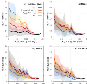
Figure 3.Relationships between many ecological variables, including NDVI, andeCO2depend highly on confounding factors. The NDVI data are partitioned into quartiles and coloured such that, ifzis the confounding variable (fractional cover, slope, aspect, or elevation), then zQ1 is the first quartile of the confounding data;zmedis the median of the confounding data; andzQ3is the third quartile. Partitioning by fractional cover yields clear separations in the response variable(a)fractional cover, as expected, since risingeCO2will have a less measurable effect on sparse vegetation within the pixel. The impact of(b)slope,(c)elevation, and(d)aspect is less clear visually, but their contribution to the model is statistically significant.

separation for fractional cover, which reinforces an expected result:eCO2had a negligible effect on vegetation indices and

other variables over bare ground but showed higher impacts on fully vegetated pixels. Therefore, we model each vegeta-tion variable,V, as

V =b1C+b2F+b3S+b4A+b5E (4)

+f (C, F, S, A, E)+ε,

where C is the elevated soil CO2 flux, F is the fractional

vegetation cover, S is the slope, A is the aspect, E is the elevation, and ε∼N 0, σ2 is random error. The function f (·)describes relationships between the predictor variables, which for this model is limited to the first-order interactions: f (C, F, S, A, E)=b6C×F+b7C×S (5)

+b8C×A+b9C×E+b10F×S+. . ..

Our hypothesis isHA:b16=0; that is, that the effect ofeCO2

on vegetation variableV is different from zero. Our null hy-pothesis is thenH0:b1=0.

Certain other confounding variables may affect the mod-elled relationships. The following scenarios and/or variables were also tested as confounders but did not affect the model

outcome: pixel position, site number, and species (plant species were estimated by performing an unsupervised clas-sification on the AVIRIS data). TheeCO2dataset was also

shifted to simulate winds and atmospheric pressure (Ogretim et al., 2013). This did not have an impact on the results.

Additionally, diurnal patterns of mountain slope air flows may dilute and enrich the bulk air mass the trees are exposed to with respect to CO2concentrations (Pypker et al., 2007).

If these air flow patterns are strong, they may drain the local CO2enhancement during morning and evening hours, when

these flow events are usually strongest. However, due to the constant nature of these localized enhanced emissions, the gradient, if it was diluted by such effects, re-establishes it-self during calmer daytime and night-time hours, as is evi-dent by the volcanically diffuse CO2emission signal being

detectable from airborne in situ measurements above the in-vestigated sites as well (Gerlach et al., 1999).

When evaluating the dynamics between different vari-ables, it is assumed that the study from which our ground measurements were derived (Werner et al., 2014), covered most of the known CO2 diffuse emission areas, and so the

con-Table 1.Data sources are shown along with the year in which they were acquired, the original resolution of the dataset, and the method by which they were resampled. All datasets were resampled to the AVIRIS resolution of 13 m.

Data source Year Original Resampling method

acquired resolution

Soil CO2flux 2011–2012 1 m Nearest neighbour

Canopy height 2017 1 m Nearest neighbour

Vegetation indices 2014 13 m Original resolution

Foliar traits 2014 13 m Original resolution

Fractional cover 2017 30 m Nearest neighbour

Biomass 2017 30 m Nearest neighbour

Evapotranspiration 2013 50 m Nearest neighbour; Ma et al. (2018) resampling

founding variables found for theeCO2points. Therefore, we

considered only control points with elevation, slope, and as-pect values, resas-pectively, between 2700 and 2950 m, less than 30◦, and less than 350◦.

3 Statistical estimation

Although the models were run for 42 explanatory variables (including additional vegetation indices, foliar traits, and other vegetation descriptors), for the sake of brevity we only present the best-performing variables (traits with significant p values are shown, and for all other variables, those with significantpvalues andR2>0.5). For the variables shown in Table 2, thepvalue of theeCO2term,b1, was, for each

model, <0.05 and in most cases0.01. The most signifi-cant predictor was determined by ordering terms bypvalues. As the confounding variables are expected to drive the behaviour of ecosystem properties, a reduced eCO2“rank”

(in terms of p value significance) does not negate the im-pact ofeCO2in the models; in fact, each ecosystem variable

was strongly influenced by increasingeCO2, given the low pvalues for theeCO2coefficient in each model. The rank of

each predictor variable is given in Table 3. Since multiplica-tive terms are allowed, two terms in a single ranking column (say, slope and fractional cover) means that the multiplication between the two terms is the term with the lowest pvalue. To reduce the complexity of the table, each variable is listed only once, in order of first appearance, whether singly or as a product.

4 Results

4.1 Structure: canopy height and biomass

Canopy height and biomass were accurately modelled with highR2, as seen in Table 2 and Fig. 4, althougheCO2was

the least significant predictor. In each case, eCO2 was still

Figure 4.Canopy height is well modelled by theeCO2model, with anR2=0.92 and the 1–1 line shown in black. However, the very tallest trees are not well captured.

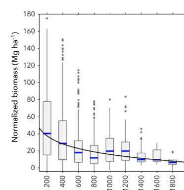
Figure 5.The biomass model prediction is shown for increasing eCO2. There is high variability at loweCO2values, but overall there is a small, but apparent, decrease in biomass with increasingeCO2.

regarded as statistically significant but had lower predictive power than the topographic variables.

Figure 5 shows the predictor variableeCO2 against the

predicted biomass. There is variability at loweCO2levels but

overall a small decrease in biomass with increasingeCO2.

This decrease appears to saturate and is better fit by a log-arithmic function; however, given that interactions between terms in the model are allowed, we do not necessarily expect a linear fit, since theeCO2 contribution to the model may

Table 2.The best-performing vegetation indices (VIs) and traits are shown with the predictive significance ofeCO₂in the model and with their correlation with a regression ensemble that included elevation, slope, aspect, and fractional cover as confounding variables (n=5520). The most significant predictor was determined by ordering terms bypvalues.

Variable Most significant Estimate for Standard error for pvalue for ModelR2

predictor term eCO₂coefficient eCO₂coefficient theeCO₂term

Structure

Canopy height Slope, FC 6e−3 1e−3 4e−6 0.92

Biomass FC 1e−1 2e−2 5e−6 0.83

Composition (vegetation indices)

Normalized difference vegetation index (NDVI) eCO₂ −6e−5 8e−6 1e−12 0.68

Red edge normalized difference VI eCO₂ −3e−5 6e−6 1e−9 0.67

Modified red edge normalized difference VI eCO₂ −7e−5 6e−6 2e−27 0.65

Vogelmann red edge index 1 eCO₂ −3e−5 1e−5 2e−3 0.64

Enhanced vegetation index eCO₂ −1e−4 1e−5 2e−22 0.62

Modified red edge simple ratio index FC −1e−4 2e−5 5e−10 0.61

Composition (plant foliar traits)

Trait: canopy nitrogen concentration Intercept −8e−3 1e−3 2e−7 0.45

Trait: carbon FC 3e−2 5e−3 5e−9 0.45

Trait: leaf mass per area (LMA) Aspect 3e−1 1e−1 6e−2 0.40

Function

Evapotranspiration (nearest neighbour) FC −8e−3 1e−3 5e−16 0.55

Evapotranspiration (statistical resampling) FC −3e−4 2e−3 8e−1 0.38

Table 3.The best-performing vegetation indices (VIs) and traits from Table 2 are shown with the ordered significance of every input into the model. Since the model allows multiplication between terms, each input is ordered by first occurrence when rankingpvalues from smallest (most significant) to largest (least significant).

Variable Ordered predictor terms (from most to least significant)

Structure

Canopy height Slope, FC Intercept Elevation eCO2 Aspect

Biomass FC Elevation Slope Intercept eCO₂ Aspect

Composition (vegetation indices)

Normalized difference vegetation index (NDVI) eCO2 FC Slope Aspect Elevation Intercept Red edge normalized difference VI eCO2, FC Aspect Slope Intercept Elevation

Modified red edge normalized difference VI eCO₂ FC, elevation Intercept Aspect Slope Vogelmann red edge index 1 eCO2, FC Intercept Aspect Elevation Slope

Enhanced vegetation index eCO2 Intercept Slope Elevation, FC Aspect

Modified red edge simple ratio index FC eCO2 Intercept Slope Aspect Elevation

Composition (plant foliar traits)

Trait: canopy nitrogen concentration Intercept eCO2, elevation FC Slope, aspect

Trait: carbon FC Elevation eCO2 Intercept Slope Aspect

Trait: leaf mass per area (LMA) Elevation FC Intercept eCO2, slope Aspect

Function

4.2 Composition: vegetation indices and foliar traits

The performance of different vegetation indices and foliar traits varied. NDVI was best modelled (R2=0.68), with eCO2as the most significant predictor (pvalue of 1×10−12).

In general, the indices were better modelled than the traits. Figure 6 shows the predicted model for NDVI (a) and the canopy nitrogen concentration trait (b) against theeCO2

pre-dictor variable. Modelled NDVI decreases with increasing eCO2, and there is a decrease in variance with increasing eCO2. The modelled canopy nitrogen concentration trait

in-creases with increasingeCO2. 4.3 Function: evapotranspiration

Canopy transpiration was relatively well represented by the eCO2 model with an R2=0.55. For comparison, total ET

was not well represented by the eCO2 model (R2=0.23),

which is sensible, as eCO2is expected to affect only plant

transpiration and not soil evaporation.eCO2was the second

most significant predictor, with fractional vegetation cover the most significant. Given that MASTER data were origi-nally acquired at a much coarser resolution (50 m) than the eCO2 ground data (1 m) and that both were resampled to

13 m resolution for a spatially consistent analysis, there may have been error introduced due to the resampling. This ef-fect is seen by the much lower model fit with the statistical resampling, although the predicted models follow the same trend. In the remainder of the paper, references to ET refer to the data resampled using nearest neighbour resampling.

Figure 7 shows the ET predicted by the model for the pre-dictor variableeCO2. There is a decrease in ET for increasing eCO2, along with a decrease in variance.

4.4 Ecosystem synergies

Given that many of the vegetation indices and traits are only appropriate in the presence of vegetation, a fractional cover threshold of 0.7 was used for theeCO2sample, for the sake

of evaluating the dynamics between modelled variables. With this threshold, only 55 data points remained, and so the sam-ple size is too small to make claims of statistical significance. Therefore, we present the following results as interesting ob-servations that may inform future data acquisition.

Figure 8 shows the dynamics between variables in the en-tire scene (i.e. non-elevated, background soil CO2) versus

the points witheCO2measurements. It is important to note

that in each sub-figure, independent data sources are used to avoid showing intrinsically correlated datasets. Fractional cover and biomass are derived from the ASO lidar data; the vegetation trait data and foliar traits are derived from AVIRIS imagery; and ET is derived from MASTER data. In this case, the variables shown are directly as observed (or derived di-rectly from the data source).

We observed interesting dynamics between ecosystem variables, suggesting great potential for future research. In theeCO2subset, NDVI was, on average, lower than that

ob-served for the same fractional cover in the control dataset (Fig. 8a). This is consistent with the model illustration of de-creased greenness for increasing eCO2. Similarly, ET was

lower in theeCO2subset for pixels with the same NDVI

ob-served in the control, showing a greater degree of stress even when plants have the same greenness (Fig. 8b). In addition, the strong linear relationship between ET and NDVI appears to break down for the points affected byeCO2.

Canopy nitrogen in theeCO2subset increased with

frac-tional cover, unlike the control, which remained flat, which again mimics the modelled data findings (Fig. 8c). ET was lower in theeCO2subset for the same biomass, which

im-plies that plants are doubly affected by the enhanced CO2

– the biomass decreases with increasingeCO2, and the ET

decreases further with decreasing biomass (Fig. 8d). Again, the strong linear relationship between ET and biomass breaks down for those points affected byeCO2. These findings

sug-gest complex relationships between ecosystem parameters in their response to increasingeCO2.

5 Discussion

Using airborne remotely sensed ecosystem properties against a ground-measured database ofeCO2(volcanic excess CO2

emanating into the forest canopy through the soil), we evalu-ated the effects of increasingeCO2on plant structure,

func-tion, and composition. Our aims were to (i) evaluate whether a passively degassing volcanic system is a viable means to study properties of ecosystems, (ii) determine if ecosystem variables are adequately detected using airborne data, and (iii) present key lessons learnt that can enable similar stud-ies over different biomes.

This study has provided initial observations of ecological responses toeCO2 that are measurable from airborne data.

We found that (a)eCO2was a significant predictor in

regres-sion ensemble models of ecosystem variables and (b) there were visual differences between the sites of increasedeCO2

and the background image. This work also demonstrates that an active volcanic system is a viable way in which to study the CO2effect on ecosystems.

The regression ensemble model showed that eCO2 was

a significant predictor for two structural variables (canopy height and biomass), nine composition variables (six veg-etation indices, three foliar traits), and a function variable (ET). Therefore, as hypothesized,eCO2 affects ecosystems

in structure, composition, and function, all of which are de-tectable both with airborne observations as well as within a volcanically derived eCO2 system. Further evaluation of

the model showed that both canopy height and biomass de-creased with increasing eCO2; the vegetation indices

Figure 6. (a)The modelled NDVI prediction is shown for predictor variableeCO2. There is a decrease in NDVI for increasingeCO2, despite larger variance at loweCO2values.(b)The modelled canopy nitrogen concentration trait prediction is shown for predictor variableeCO2. There is a clear increase in canopy nitrogen concentration with increasingeCO2.

Figure 7.The normalized canopy transpiration prediction is shown against predictor variable eCO2, for training data with nearest neighbour resampling. There is a clear decrease in ET for increasing eCO2, with larger variance at loweCO2values.

increases; LMA decreases; carbon decreases; and ET de-creases.

Some of these observations contrasted with results found in other published studies, while others agreed. For instance, our study found a decrease in NDVI with increasingeCO2,

which correlates to the multispectral satellite findings of Rouse et al. (2010) and Cholathat et al. (2011). In some cases, the decrease others have found can be explained by the tree-kill effect, where vegetation is removed. However, by ac-counting for fractional cover in our models, we have shown that NDVI decreases independently of fractional cover (see

in Fig. 8). This shows that, regardless of whether the number of trees changes, the greenness of individual trees is reduced. This finding is in direct contrast with the CO2fertilization

hypothesis, which states that rising CO2has a positive effect

on plant growth and productivity due to increased availability of carbon, which has been shown using field data (Zhu et al., 2016; Huang et al., 2007). However, this decrease in NDVI could also be explained by a reduction in leaves, rather than a reduction in leaf health, due to more efficient leaves (e.g. higher nutrient concentration, more efficient in water use).

The decrease in canopy height and biomass agrees with the tree-ring study done by Biondi and Fessenden (1999), which also found slower lodgepole pine growth rates in high CO2 emission areas on Mammoth Mountain. However, a

study by Smith et al. (2013) found an increase in biomass in the mixed-species temperate forest FACE experiment. In that experiment, there was large variation between and within species, and the experiment was limited to 4 years. Perhaps a long-term species composition shift due toeCO2was the

cause of the change in biomass in our study, but we do not have individual tree species-level data to support this hypoth-esis.

and a study of ice cores showed a 40 % decrease in stom-atal density over the last 200 years, which parallelled an in-crease in global CO2(Woodward, 1987). However, Sharma

and Williams (2009) evaluated vegetation naturally exposed to CO2in Yellowstone National Park and found reduced

ni-trogen at a leaf level inPinus contorta(lodgepole pine) and increased nitrogen at a leaf level forLinaria dalmatica (Dal-mation toadflax; an invasive, non-native herb). Once again, the species-level differences highlight the need for remote-sensing analysis over areas that encompass wide species vari-ation, in order to understand overall trends.

Kimball et al. (1998) found a slight increase in ET in a FACE experiment over cotton fields, but that increase was within the error of the ET estimation and so was not deemed statistically significant. In contrast, Nendel et al. (2009) found a decrease in ET and an increase in dry above-ground biomass over a FACE crop rotation experiment. In this study, we found a decrease in ET. In addition, we found a decrease in ET relative to both NDVI and biomass, when comparing the points affected byeCO2to those unaffected points in the

surrounding area. The unaffected sites showed a positive lin-ear relationship between ET and both NDVI and biomass, which appeared to break down for points affected byeCO2

in both relationships.

The combination of lower NDVI, higher canopy nitrogen, and higher ET suggests a canopy that uses less water with rising CO2 resulting in higher water use efficiency, with a

nutrient-rich canopy. Since leaves are stronger and more effi-cient, fewer are required for photosynthesis. While biomass increased slightly, the more obvious change was the decrease in the variance of biomass, which points to alignment to more similar trees with elevated CO2.

High fluxes of CO2 through soils in kill zones on

Mam-moth Mountain have likely impacted forest ecosystems through oxygen deprivation in soil pore space, inhibition of root respiration, and soil acidification (McGee and Gerlach, 1998; Farrar et al., 1995; Qi et al., 1994). Since we used soil CO2flux as the predictor variable in the model, some of the

observed ecosystem responses may therefore be due to the effects of high concentrations of CO2 on the soil

environ-ment or some combination of soil and atmospheric effects. However, by using fractional cover as an input to the model and excluding the kill zones altogether to derive Figure 8, we are focusing on the CO2gradient over vegetated areas around

these zones, that are unlikely to be affected by soil acidifica-tion. The Mammoth Mountain soil CO2 flux dataset does,

however, provide a record of CO2emissions that is more

sta-ble in space and time than measurements of atmospheric CO2

concentrations. In particular, forest canopies will through time be exposed to eCO2at highly variable levels because

the originally mostly invariant eCO2 once emitted through

the soil into the sub-canopy atmosphere is subject to highly variable dispersion from thermal and wind disturbances at minute, diurnal, and seasonal scales (Staebler and Fitzjar-rald, 2004). In-canopy concentration measurements ofeCO2

will therefore be highly variable, and, especially if conducted instantaneously, may not be representative of the long-term relative exposure strength in the canopy.

Vegetation at this site is also responding to the partial pres-sure of CO2 in the atmosphere, among other gases. A

re-sponse above the asymptote of the net photosynthetic rate versus internal CO2partial pressure (A-Ci curve) would

re-sult in very little vegetation response to the partial pressures (Tissue et al., 1999). However, the partial pressures even at elevated molar concentration at Mammoth are about 60 % of those at sea level. The fact that we see systematic ecosystem effects suggests that elevation is not on the flat part of the A-Ci curve. In other words, even if elevation were to reduce the CO2effect, we still are seeing strong CO2effects

regard-less, highlighting just how important and strong of a response we are able to detect.

We will clarify that the effects should not necessarily be given a subjective description of “negative”; rather, it is im-portant to note that the CO2fertilization effect is unlikely to

continue indefinitely, particularly at the same rates that FACE studies have shown only in the short term. All other experi-ments have been unable to show long-term effects. Our study suggests that over the scale of decades, some of these hypoth-esized greening or biomass increases may not be sustainable. Other results, such as an increase in canopy nitrogen with in-creasing CO2, do seem to remain consistent with our study,

however.

This exploratory study leveraged existing data acquired over Mammoth Mountain. We used ASO lidar, AVIRIS, and MASTER data to derive products that describe ecosystem structure, composition, and function and used field eCO2

measurements to show that elevated CO2was a significant

predictor of ecosystem variables, including vegetation in-dices, plant foliar traits, biomass, and evapotranspiration. While our study has shown the promise of airborne remote sensing in detecting measurable ecosystem changes in forest ecosystems on and around a CO2-emitting volcanic system,

it was also completed using an existing ad hoc collection of data. The nature of the collection of data sources enabled us to understand the details of the data characteristics necessary for future studies.

While this study is useful for showing the benefit of both a passively emitting volcanic system and airborne data for evaluating the ecosystem response to eCO2, we anticipate

analysis. We note that this study was exploratory and that this study was intended to identify both potential signals as well as design elements for further study.

6 Conclusions

This exploratory study used airborne remote-sensing data, coupled with ground measurements of volcanic soil CO2flux

on a forested volcano, to derive relationships between ris-ing CO2 emissions and ecosystem structure, function, and

composition metrics. We have shown that passively emitting volcanic systems are viable environments in which to study CO2impacts on ecosystems, witheCO2the most significant

predictor in regression ensemble models of several ecolog-ical variables, including NDVI, canopy nitrogen concentra-tion, ET, and biomass. When comparing differences between vegetation parameters affected byeCO2and those estimated

over the background scene, we found contrasting patterns and dynamics between ecological variables, showing that a combination of different remote-sensing platforms is capable of providing a comprehensive view of ecosystem responses to long-term elevated volcanic CO2.

Key lessons learnt from this study include the following: 1. Future campaigns should acquire all data at the same or

similar resolution at individual tree scale.

2. Significantly more than 55 vegetated tree points are necessary in order to draw meaningful conclusions re-garding the dynamics between variables at Mammoth Mountain (which has one dominant tree species). The number of required points in other environments will vary according to ecosystem complexity and will likely far exceed this number.

3. Combining lidar and spectral data across a range of wavelengths yielded a more complete view than using any one data source alone.

Data availability. Soil CO2data are the property of the USGS and may be requested through Cynthia Werner at the USGS. AVIRIS data are available by searching for flight line f141021t01p00r05 at https://aviris.jpl.nasa.gov/alt_locator/ (AVIRIS Data Portal, 2018). MASTER data are available via https://masterprojects.jpl.nasa.gov/ L2_Products (MASTER Data Products, 2018). The flight ID is 14-903-00; line 02. Lidar data used in this study are the property of the Airborne Snow Observatory and may be obtained through Kat Bormann at JPL.

Competing interests. The authors declare that they have no conflict of interest.

Acknowledgements. We thank Cynthia Werner for providing soil CO2 flux data over our study area; Gregory Halverson for

processing ET data; Zhiwei Ye for processing functional trait data; and Anthony Bloom, Stuart Wilkinson, Christoph Kern, and Deborah Bergfeld for discussions during earlier stages of this project. The research described in this paper was carried out at the Jet Propulsion Laboratory, California Institute of Technology, under contract with the National Aeronautics and Space Administration. Government sponsorship acknowledged.

Edited by: Jochen Schöngart

Reviewed by: two anonymous referees

References

Anderson, D. E. and Farrar, C. D.: Eddy covariance measurement of CO2flux to the atmosphere from an area of high volcanogenic emissions, Mammoth Mountain, California, Chem. Geol., 177, 31–42, 2001.

AVIRIS Data Portal: Jet Propulsion Laboratory, California Insti-tute of Technology, available at: https://aviris.jpl.nasa.gov/alt_ locator/, last access: 13 December 2018.

Biondi, F. and Fessenden, J. E.: Response of Lodgepole Pine growth to CO2degassing at Mammoth Mountain, California, Ecology, 80, 2420–2426, 1999.

Boudoire, G., Di Muro, A., Liuzzo, M., Ferrazzini, V., Peltier, A., Gurrieri, S., Michon, L., Giudice, G., Kowalski, P., and Boissier, P.: New perspectives on volcano monitoring in a tropical envi-ronment: Continuous measurements of soil CO2flux at Piton de la Fournaise (La Réunion Island, France), Geophys. Res. Lett., 44, 8244–8253, 2017.

Camarda, M., De Gregorio, S., and Gurrieri, S.: Magma-ascent pro-cesses during 2005–2009 at Mt. Etna inferred by soil CO2 emis-sions in peripheral areas of the volcano, Chem. Geol., 330, 218– 227, 2012.

Cardellini, C., Chiodini, G., and Frondini, F.: Application of stochastic simulation to CO2 flux from soil: mapping and quantification of gas release, J. Geophys. Res., 108, 2425, https://doi.org/10.1029/2002JB002165, 2013.

Cholathat, R., Li, X., and Ge, L.: Monitoring natural analog of ge-ologic carbon sequestration using multi-temporal Landsat TM images in Mammoth Mountain, Long Valley Cadera, California, Int. Geosci. Remote Se., Vancouver, 24–29 July 2011, 2011. Cook, A. C., Hainsworth, L. J., Sorey, M. L., Evans, W. C., and

Southon, J. R.: Radiocarbon studies of plant leaves and tree rings from Mammoth Mountain, CA: a long-term record of magmatic CO2release, Chem. Geol., 177, 117–131, 2001.

Drake, B. G., Gonzàlez-Meler, M. A., and Long, S. P.: More Efficient Plants: A Consequence of Rising At-mospheric CO2?, Annu. Rev. Plant Phys., 48, 609–639, https://doi.org/10.1146/annurev.arplant.48.1.609, 1997. Evans, J. S. and Hudak, A. T.: A multiscale curvature

al-gorithm for classifying discrete return LiDAR in forested environments, IEEE T. Geosci. Remote, 45, 1029–1038, https://doi.org/10.1109/TGRS.2006.890412, 2007.

Fisher, J. B., and ECOSTRESS Algorithm Development Team: ECOsystem Spaceborne Thermal Radiometer Experiment on Space Station (ECOSTRESS): Level-3 Evapotranspiration Algo-rithm Theoretical Basis Document, 24 pp, Jet Propulsion Labo-ratory, Pasadena, 2015.

Fisher, J. B., Melton, F., Middleton, E., Hain, C., Anderson, M., Allen, R., McCabe, M. F., Hook, Baldocchi, D., Townsend, P. A., Kilic, A., Tu, K., Miralles, D. D., Perret, J., Lagouarde, J.-P., Waliser, D., Purdy, A. J., French, A., Schimel, D., Famiglietti, J. S., Stephens, G., and Wood, E. F.: The Future of Evapotranspi-ration: Global requirements for ecosystem functioning, carbon and climate feedbacks, agricultural management, and water re-sources, Water Resour. Res., 53, 2618–2626, 2017.

Fisher, J. B., Tu, K., Baldocchi, D. D.: Global estimates of the land-atmosphere water flux based on monthly AVHRR and ISLSCP-II data, validated at 16 FLUXNET sites, Remote Sens. Environ., 112, 901–919, 2008.

Friedlingstein, P., Meinshausen, M., Arora, V. K., Jones, C. D., Anav, A., Liddicoat, S. K., and Knutti, R.: Uncertainties in CMIP5 Climate Projections due to Carbon Cycle Feedbacks, J. Climate, 27, 512–526, 2014.

Garcia, M., Saatchi, S., Ferraz, A., Silva, C.A., Ustin, S., Koltunov, A., and Balzter, H.: Impact of data model and point density on aboveground forest biomass estimation from airborne LiDAR, Carbon Balance and Management, 12, 4, https://doi.org/10.1186/s13021-017-0073-1, 2017.

Gerlach, T. M.: Present-day CO2 emissions from volcanos, Eos Trans. AGU, 72, 249–255, https://doi.org/10.1029/90EO10192, 1991.

Gerlach, T. M., Doukas, M. P., McGee, K. A., and Kessler, R.: Air-borne detection of diffuse carbon dioxide emissions at Mammoth Mountain, California, Geophys. Res. Lett., 26, 3661–3664, 1999. Giammanco, S., Sims, K. W. W., and Neri, M.: Measurements of 220Rn and 222Rn and CO2 emissions in soil and fumarole gases on Mt. Etna volcano (Italy): Implications for gas transport and shallow ground fracture, Geochem. Geophy. Geosy., 8, 10, https://doi.org/10.1029/2007GC001644, 2007.

Gillespie, A., Rokugawa, S., Matsunaga, T., Cothern, J. S., Hook, S. J., and Kahle, A. B.: A temperature and emissivity separa-tion algorithm for Advanced Spaceborne Thermal Emission and Relection Radiometer (ASTER) images, IEEE T. Geosci. Re-mote Sens., 36, 1113–1126, 1998.

Hernández, P. A., Pérez, N. M., Salazar, J. M., Nakai, S., Notsu, K., and Wakita, H.: Diffuse emission of carbon dioxide, methane, and helium-3 from Teide Volcano, Tener-ife, Canary Islands, Geophys. Res. Lett., 25, 3311–3314, https://doi.org/10.1029/98GL02561, 1998.

Huang, J.-G., Bergeron, Y., Denneler, B., Berninger, F., and Tardif, J.: Response of forest trees to increased at-mospheric CO2, Crit. Rev. Plant Sci., 26, 265–283, https://doi.org/10.1080/07352680701626978, 2007.

Kerrick, D. M.: Present and past nonanthropogenic CO2 de-gassing from the solid earth, Rev. Geophys., 39, 565–585. https://doi.org/10.1029/2001RG000105, 2001.

Kimball, B. A, LaMorte, R. L., Seay, R. S., Pinter Jr, P. J., Rokey, R. R., Hunsaker, D. J., Dugas, W. A., Heuer, M. L., Mauney, J. R., Hendrey, G. R., Lewin, K. F., and Nagy, J.: Effects of free-air CO2enrichment on energy balance and evapotranspiration of cotton, Agr. Forest Meteorol., 70, 259–278, 1998.

Kobayashi, H. and Iwabuchi, H.: A coupled 1-D atmosphere and 3-D canopy radiative transfer model for canopy reflectance, light environment, and photosynthesis simulation in a heterogeneous landscape, Remote Sens. Environ., 112, 173–185, 2008. Kolby Smith, W., Reed, S. C., Cleveland, C. C., Ballantyne, A.

P., Anderegg, W. R. L., Wieder, W. R., and Running, S. W.: Large divergence of satellite and Earth system model estimates of global terrestrial CO2fertilization, Nat. Clim. Change, 6, 306– 310, https://doi.org/10.1038/nclimate2879, 2015.

Körner, C.: Plant CO2 responses: an issue of definition, time and resource supply, New Phytol., 172, 393–411, https://doi.org/10.1111/j.1469-8137.2006.01886.x, 2006. Le Quéré, C., Andrew, R. M., Canadell, J. G., Sitch, S.,

Kors-bakken, J. I., Peters, G. P., Manning, A. C., Boden, T. A., Tans, P. P., Houghton, R. A., Keeling, R. F., Alin, S., Andrews, O. D., Anthoni, P., Barbero, L., Bopp, L., Chevallier, F., Chini, L. P., Ciais, P., Currie, K., Delire, C., Doney, S. C., Friedlingstein, P., Gkritzalis, T., Harris, I., Hauck, J., Haverd, V., Hoppema, M., Klein Goldewijk, K., Jain, A. K., Kato, E., Körtzinger, A., Land-schützer, P., Lefèvre, N., Lenton, A., Lienert, S., Lombardozzi, D., Melton, J. R., Metzl, N., Millero, F., Monteiro, P. M. S., Munro, D. R., Nabel, J. E. M. S., Nakaoka, S.-I., O’Brien, K., Olsen, A., Omar, A. M., Ono, T., Pierrot, D., Poulter, B., Röden-beck, C., Salisbury, J., Schuster, U., Schwinger, J., Séférian, R., Skjelvan, I., Stocker, B. D., Sutton, A. J., Takahashi, T., Tian, H., Tilbrook, B., van der Laan-Luijkx, I. T., van der Werf, G. R., Viovy, N., Walker, A. P., Wiltshire, A. J., and Zaehle, S.: Global Carbon Budget 2016, Earth Syst. Sci. Data, 8, 605–649, https://doi.org/10.5194/essd-8-605-2016, 2016.

Lewicki, J. L., Hilley, G. E., Tosha, T., Aoyagi, R., Ya-mamoto, K., and Benson, S. M.: Dynamic coupling of vol-canic CO2 flow and wind at the HorseshoeLake tree kill, Mammoth Mountain, CA, Geophys. Res. Lett., 34, L03401, https://doi.org/10.1029/2006GL028848, 2006.

Lewicki, J. L., Hilley, G. E., Tosha, T., Aoyagi, R., Ya-mamoto, K., and Benson, S. M.: Dynamic coupling of volcanic CO₂ flow and wind at the Horseshoe Lake tree kill, Mam-moth Mountain, California, Geophys. Res. Lett., 34, L03401, https://doi.org/10.1029/2006GL028848, 2007.

Lewicki, J. L., Fischer, M. L., and Hilley, G. E.: Six-week time series of eddy covariance CO2 flux at Mammoth Moun-tain, California: performance evaluation and role of mete-orological forcing, J. Volcanol. Geoth. Res., 171, 178–190, https://doi.org/10.1016/j.jvolgeores.2007.11.029, 2008. Lewicki, J. L., Hilley, G. E., Dobeck, L., and Marino, B. D.: Eddy

covariance imaging of diffuse volcanic CO2emissions at Mam-moth Mountain, CA, USA, Bull. Volcanol., 74, 135–141, 2012. Lewicki, J. L. and Hilley, G. E.: Multi-scale observations

of the variability of magmatic CO2 emissions, Mammoth Mountain, CA, USA, J. Volcanol. Geoth. Res., 284, 1–15, https://doi.org/10.1016/j.jvolgeores.2014.07.011, 2014. Lewicki, J. L., Hilley, G. E., Shelly, D. R., King, J. C., McGeehin,

J. P., and Mangan, M.: Crustal migration of CO₂-rich magmatic fluids recorded by tree-ring radiocarbon and seismicity at Mam-moth Mountain, CA, USA, Earth Planet. Sci. Lett., 390, 52–58, 2014.

diox-ide enrichment facility, Agric. Forest Meteorol., 70, 15–29, https://doi.org/10.1016/0168-1923(94)90045-0, 1994.

List, M. R.: Geologic remote sensing and GIS evaluation of vol-canogenic CO2-induced tree kills: Mammoth Mountain, Califor-nia, 1991–2004, M.S. Thesis, CSUS, 2005.

Ma, P., Kang, E. L., Braverman, A., and Nguyen, H.: Spatial sta-tistical downscaling for constructing high-resolution nature runs in global observing system simulation experiments, in review, 2018.

Mason, E., Edmonds, M., and Turchyn, A. V.: Remobilization of crustal carbon may dominate volcanic arc emissions, Science, 357, 290–294, 2017.

MASTER Data Products: Jet Propulsion Laboratory, California Institute of Technology, available at: https://masterprojects.jpl. nasa.gov/L2_Products/, last access: 13 December 2018. McGee, K. A. and Gerlach, T. M.: Annual cycle of

mag-matic CO2 in a tree-kill soil at Mammoth Moun-tain, California: Implications for soil acidification, Geology, 26, 463–466, https://doi.org/10.1130/0091-7613(1998)026<0463:ACOMCI>2.3.CO;2, 1998.

McGuire, A. D., Melillo, J. M., and Joyce, L. A.: The Role of Ni-trogen in the Response of Forest Net Primary Production to Ele-vated Atmospheric Carbon Dioxide, Annu. Rev. Ecol. Syst., 26, 473–503, 1995.

Nendel, C., Kersebaum, K. C., Mirschel, W., Manderscheid, R., Weigel, H.-J., and Wenkel, K.-O.: Testing different CO2response algorithms against a FACE crop rotation experiment, NJAS – Wageningen, J. Life Sci., 57, 17–25, 2009.

Norby, R. J., De Kauwe, M. G., Domingues, T. F., Duursma, R. A., Ellsworth, D. S., Goll, D. S., and Zaehle, S.: Model– data synthesis for the next generation of forest free-air CO2 enrichment (FACE) experiments, New Phytol., 209, 17–28, https://doi.org/10.1111/nph.13593, 2016.

Ogretim, E., Crandall, D., Gray, D. D., and Bromhai, G. S.: Ef-fects of Atmospheric Dynamics on CO₂Seepage at Mammoth Mountain, California USA, Journal of Computational Multi-phase Flows, 5, 283–294, 2013.

Painter, T. H., Berisford, D. F., Boardman, J. W., Bormann, K. J., Deems, J. S., Gehrke, F., Hedrick, A., Joyce, M., Laidlaw, R., Marks, D., Mattmann, C., McGurk, B., Ramirez, P., Richardson, M., Skiles, S. M., Seidel, F. C., and Winstral, A.: The Airborne Snow Observatory: Fusion of scanning lidar, imaging spectrom-eter, and physically-based modeling for mapping snow water equivalent and snow albedo, Remote Sens. Environ., 184, 139– 152. https://doi.org/10.1016/j.rse.2016.06.018, 2016.

Perez, N. M., Hernandez, P. A., Padilla, G., Nolasco, D., Barran-cos, J., Melian, G., and Ibarra, M.: Global CO2emission from volcanic lakes, Geology, 39, 235–238, 2011.

Peterson, B. J. and Melillo, J. M.: The potential storage of carbon caused by eutrophication of the biosphere, Tellus B, 37, 117–127, https://doi.org/10.1111/j.1600-0889.1985.tb00060.x, 1985. Pickles, W. L., Kasameyer, P. W., Martini, B. A., Potts, D. C., and

Silver, E. A.: Geobotanical Remote Sensing for Geothermal Ex-ploration, Geothermal Resources Council 2001 Annual Meeting, San Diego, California, 26–29 August, 2001.

Potter, D. A.: Forested Communities of the Upper Montane in the Central and Southern Sierra Nevada, United States Department of Agriculture General Technical Report PSW-GTR-169, 1998.

Pypker, T. G., Unsworth, M. H., Mix, A. C., Rugh, W., Ocheltree, T., Alstad, K., and Bond, B. J.: Using Nocturnal Cold Air Drainage Flow to Monitor Ecosystem Processes in Complex Terrain, Ecol. Appl., 17, 702–714, 2007.

Qi, J., Marshall, J. D., and Mattson, K. G.: High soil carbon dioxide concentrations inhibit root respiration of Douglas fir, New Phy-tol., 128, 435–442, 1994.

Rahn, T. A., Fessenden, J. E., and Wahlen, M.: Flux chamber mea-surements of anomalous CO2emission from the flanks of Mam-moth Mountain, California, Geophys. Res. Lett., 23, 1861–1864, 1996.

RiANALYZE: available at: http://www.riegl.com/products/ software-packages/rianalyze/, last access: 8 July 2017.

Rouse, J. H., Shaw, J. A., Lawrence, R. L., Lewicki, J. L., Dobeck, L. M., Repasky, K. S., and Spangler, L. H.: Multi-spectral imag-ing of vegetation for detectimag-ing CO2leaking from underground, Environ. Earth Sci., 60, 313–323, 2010.

Ryu, Y., Baldocchi, D. D, Kobayashi, H., van Ingen, C., Li, J., Black, T. A., Beringer, J., van Gorsel, E., Knohl, A., Law, B. E., and Roupsard, O.: Integration of MODIS land and atmosphere products with a coupled-process model to esti-mate gross primary productivity and evapotranspiration from 1 km to global scales, Global Biogeochem. Cy., 25, GB4017, https://doi.org/10.1029/2011GB004053, 2011.

Schimel, D. S.: Terrestrial ecosystems and the carbon cycle, Glob. Change Biol., 1, 77–91, https://doi.org/10.1111/j.1365-2486.1995.tb00008.x, 1995.

Schimel, D., Stephens, B. B., and Fisher, J. B.: Effect of increasing CO2on the terrestrial carbon cycle, P. Natl. Acad. Sci. USA, 112, 436–441. https://doi.org/10.1073/pnas.1407302112, 2015. Schwandner, F. M., Gunson, M. R., Miller, C. E., Carn, S. A.,

El-dering, A., Krings, T., and Podolske, J. R.: Spaceborne detection of localized carbon dioxide sources, Science, 358, eaam5782, https://doi.org/10.1126/science.aam5782, 2017.

Schwandner, F. M., Seward, T. M., Gize, A. P., Hall, P. A., and Di-etrich, V. J.: Diffuse emission of organic trace gases from the flank and crater of a quiescent active volcano (Vulcano, Ae-olian Islands, Italy), J. Geophys. Res.-Atmos., 109, D04301, https://doi.org/10.1029/2003JD003890, 2004.

Sharma, S. and Williams, D. G.: Carbon and oxygen isotope analy-sis of leaf biomass reveals contrasting photosynthetic responses to elevated CO2 near geologic vents in Yellowstone National Park, Biogeosciences, 6, 25–31, https://doi.org/10.5194/bg-6-25-2009, 2009.

Singh, A., Serbin, S. P., McNeil, B. E., Kingdon, C. C., and Townsend, P. A.: Imaging spectroscopy algorithms for mapping canopy foliar chemical and morphological traits and their uncer-tainties, Ecol. Appl., 25, 2180–2197, 2015.

Smith, A. R., Lukac, M., Hood, R., Healey, J. R., Miglietta, F., and Godbold, D. L.: Elevated CO2enrichment induces a differential biomass response in a mixed species temperate forest plantation, New Phytol., 198, 156–168, 2013.

Sorey, M. L., Evans, W. C., Kennedy, B. M., Farrar, C. D., Hainsworth, L. J., and Hausback, B.: Carbon dioxide and helium emissions from a reservoir of magmatic gas beneath Mammoth Mountain, California, J. Geophys. Res.-Sol. Ea, 103, 15303– 15323, 1998.

Tercek, M. T., Al-Niemi, T. S., and Stout, R. G.: High Levels of Carbon Dioxide in YellowStone National Park: A Glimpse into the Future?, Yellowstone Science, 16, 12–19, 2008.

Thenkabail, P. S., Lyon, J. G., and Huete, A.: Hyperspectral Remote Sensing of Vegetation, CRC Press, Taylor and Francis Group, 405–406, 2016.

Thompson, D. R., Gao, B.-C., Green, R. O., Roberts, D. A., Den-nison, P. E., and Lundeen, S. R.: Atmospheric correction for global mapping spectroscopy: ATREM advances for the HyspIRI preparatory campaign, Remote Sens. Environ., 167, 64–77, 2015. Tissue, D. T., Griffin, K. L., and Ball, J. T.: “Photosynthetic Ad-justment in Field-Grown Ponderosa Pine Trees after Six Years of Exposure to Elevated CO2”, Tree Physiol., 19, Oxford University Press, 221–228, 1999.

Tonooka, H.: Accurate Atmospheric Correction of ASTER Thermal Infrared Imagery Using the WVS Method, IEEE Trans. Geos. Remote Sens., 43, 2778–2792, 2005.

Verma, M., Fisher, J. B., Mallick, K., Ryu, Y., Kobayashi, H., Guil-laume, A., Moore, G., Ramakrishnan, L., Hendrix, V., Wolf, S., Sikka, M., Kiely, G., Wohlfahrt, G., Gielen, B., Roupsard, O., Toscano, P., Arain, M. A., and Cescatti, A.: Global surface net-radiation at 5 km from MODIS Terra, Remote Sens., 8, 1–20, 2016.

Werner, C. and Brantley, S.: CO2 emissions from the Yellow-stone volcanic system, Geochem. Geophy. Geosy., 4, 1061, https://doi.org/10.1029/2002GC000473, 2003.

Werner, C., Bergfeld, D., Farrar, C. D., Doukas, M. P., Kelly, P. J., and Kern, C.: Decadal-scale variability of dif-fuse CO2 emissions and seismicity revealed from long-term monitoring (1995–2013) at Mammoth Mountain, Cal-ifornia, USA, J. Volcanol. Geotherm. Res., 289, 51–63, https://doi.org/10.1016/j.jvolgeores.2014.10.020, 2014. Woodward, F. I.: Stomatal numbers are sensitive to increases in CO2

from pre-industrial levels, Nature, 327, 617–618, 1987. Zhu, Z., Piao, S., Myneni, R. B., Huang, M., Zeng, Z., Canadell,