HARP: A MACHINE LEARNING FRAMEWORK ON TOP OF THE COLLECTIVE COMMUNICATION LAYER FOR THE BIG DATA SOFTWARE STACK

HARP: A MACHINE LEARNING FRAMEWORK

ON TOP OF THE COLLECTIVE COMMUNICATION LAYER

FOR THE BIG DATA SOFTWARE STACK

Bingjing Zhang

Submitted to the faculty of the University Graduate School in partial fulfillment of the requirements

for the degree Doctor of Philosophy

in the School of Informatics and Computing, Indiana University

Accepted by the Graduate Faculty, Indiana University, in partial fulfillment of the requirements for

the degree of Doctor of Philosophy.

Doctoral Committee

Judy Qiu, Ph.D.

Geoffrey Charles Fox, Ph.D.

David J Crandall, Ph.D.

Paul Purdom, Ph.D.

Acknowledgments

I sincerely thank my advisor, Dr. Qiu, and my colleagues: Dr. Peng, Dr. Chen, Meng Li, Yiming

Zou, Thomas Wiggins, and Allan Streib for their support to my research work. I also thank Dr.

Crandall, Dr. Fox, and Dr. Purdom, my research committee members, for providing guidance in

my thesis research. I am very grateful to my wife, Jane, and my parents for their love and support,

Bingjing Zhang

HARP: A MACHINE LEARNING FRAMEWORK ON TOP OF THE COLLECTIVE

COMMUNICATION LAYER FOR THE BIG DATA SOFTWARE STACK

Almost every field of science is now undergoing a data-driven revolution requiring analyzing

mas-sive datasets. Machine learning algorithms are widely used to find meaning in a given dataset and

discover properties of complex systems. At the same time, the landscape of computing has evolved

towards computers exhibiting many-core architectures of increasing complexity. However, there is

no simple and unified programming framework allowing for these machine learning applications

to exploit these new machines’ parallel computing capability. Instead, many efforts focus on

spe-cialized ways to speed up individual algorithms. In this thesis, the Harp framework, which uses

collective communication techniques, is prototyped to improve the performance of data movement

and provides high-level APIs for various synchronization patterns in iterative computation.

In contrast to traditional parallelization strategies that focus on handling high volume training

data, a less known challenge is that the high dimensional model is also in high volume and

diffi-cult to synchronize. As an extension of the Hadoop MapReduce system, Harp includes a collective

communication layer and a set of programming interfaces. Iterative machine learning algorithms

can be parallelized through efficient synchronization methods utilizing both inter-node and

intra-node parallelism. The usability and efficiency of Harp’s approach is validated on applications such

as K-means Clustering, Multi-Dimensional Scaling, Latent Dirichlet Allocation and Matrix

Fac-torization. The results show that these machine learning applications can achieve high parallel

performance on Harp.

Judy Qiu, Ph.D.

Geoffrey Charles Fox, Ph.D.

David J Crandall, Ph.D.

Contents

1 Introduction 1

2 Machine Learning Algorithms & Computation Models 6

2.1 Machine Learning Algorithms . . . 6

2.2 Computation Model Survey . . . 7

2.3 Latent Dirichlet Allocation . . . 10

2.3.1 LDA Background . . . 11

2.3.2 Big Model Problem . . . 14

2.3.3 Model Synchronization Optimizations . . . 17

2.3.4 Experiments . . . 19

3 Solving Big Data Problem with HPC Methods 26 3.1 Related Work . . . 26

3.2 Research Methodologies . . . 29

4 Harp Programming Model 32 4.1 MapCollective Programming Model . . . 32

4.2 Hierarchical Data Interfaces . . . 32

4.3 Collective Communication Operations . . . 34

4.4 Mapping Computation Models to Harp Programming Interfaces . . . 37

5 Harp Framework Design and Implementation 39 5.1 Layered Architecture . . . 39

5.2 Data Interface Methods . . . 39

5.3 Collective Communication Implementation . . . 43

5.4 Intra-Worker Scheduling and Multi-Threading . . . 44

7.2 WDA-SMACOF . . . 52

8 The Rotation-based Solution 53 8.1 Algorithms . . . 54

8.2 Programming Interface and Implementation . . . 56

8.2.1 Data Abstraction and Execution Flow . . . 56

8.2.2 Pipelining and Dynamic Rotation Control . . . 57

8.2.3 Algorithm Parallelization . . . 61

8.3 Experiments . . . 62

8.3.1 Experiment Settings . . . 62

8.3.2 LDA Performance Results . . . 63

8.3.3 MF Performance Results . . . 68

9 Conclusion 72

References 74

1 Introduction

Data analytics is undergoing a revolution in many scientific domains. Machine learning algorithms1

have become popular methods for analytics, which allow computers to learn from existing data

and make data-based predictions. They have been widely used in computer vision, text mining,

advertising, recommender systems, network analysis, and genetics. Unfortunately, analyzing big

data usually exceeds the capability of a single or even a few machines owing to the incredible

volume of data available, and thus requires algorithm parallelization at an unprecedented scale.

Scaling up these algorithms is challenging because of their prohibitive computation cost, not only

the need to process enormous training data in iterations, but also the requirement to synchronize big

models in rounds for algorithm convergence.

Through examining existing parallel machine learning implementations, I conclude that the

parallelization solutions can be categorized into four types of computation models: “Locking”,

“Rotation”, “Allreduce”, and “Asynchronous”. My classification of the computation models is based

on model synchronization patterns (synchronized algorithms or asynchronous algorithms) and the

effectiveness of the model parameter update (the latest model parameters or stale model parameters).

As a particular case study, I chose a representative machine learning algorithm, Collapsed Gibbs

Sampling (CGS) [1, 2] for Latent Dirichlet Allocation (LDA) [3], to understand the differences

between these computation models. LDA is a widely used machine learning technique for big

data analysis. It includes an inference algorithm that iteratively updates a model until the model

converges. The LDA application is commonly solved by the CGS algorithm. A major challenge is

the scaling issue in parallelization owing to the fact that the model size is huge, and parallel workers

need to communicate the model parameters continually. I identify three important features of the

parallel LDA computation to consider here:

1. The volume of model parameters required for the local computation is high

2. The time complexity of local computation is proportional to the required model size

3. The model size shrinks as it converges

In the LDA parallelization, compared with the “Asynchronous” computation model, the “Allreduce”

computation model with optimized communication routing can improve the model synchronization

speed, thus allowing the model to converge faster. This performance improvement derives not only

from accelerated communication but also from reduced iteration computation time as the model

size shrinks during convergence. The results also reveal that the “Rotation” computation model can

achieve faster model convergence speed than the “Allreduce” computation model. The main

ratio-nale is that in the training procedure running on each worker, the “Allreduce” computation model

uses stale model parameters, but the “Rotation” computation model uses the latest model

parame-ters. The effect of the model update in convergence reduces when stale model parameters are used.

Besides, even when two implementations use the “Rotation” computation model, communication

through sending model parameters in chunks can further reduce communication overhead compared

with flooding small messages.

Synchronized communication performed by all the parallel workers is referred to as “collective

communication” in the High-Performance Computing (HPC) domain. In MPI [4], some collective

communication patterns are implemented with various optimizations and invoked as operations.

Though the collective communication technique can result in efficient model synchronization as is

shown in LDA, it has not been thoroughly applied to many machine learning applications. MPI only

provides basic collective communication operations which describe process-to-process

synchro-nization patterns, so it does not cover all the complicated parameter-to-parameter synchrosynchro-nization

patterns. In that case, users have to rely on send/receive calls to develop those customized

synchro-nization patterns. The applications developed achieve high performance but create a complicated

code base.

Another way to implement machine learning algorithms is to use big data tools. Initially, many

machine learning algorithms were implemented in MapReduce [5, 6]. However, these

implementa-tions suffer from repeated input data loading from the distributed file systems and slow disk-based

intermediate data synchronization in the shuffling phase. This motivates the design of iterative

MapReduce tools such as Twister [7] and Spark [8], which utilizes memory for data caching and

communication and thus drastically improve the performance of large-scale data processing. Later,

big data tools have expanded rapidly and form an open-source software stack. Their programming

models are not limited to MapReduce and iterative MapReduce. In graph processing tools [9],

in-put data are abstracted as a graph and processed in iterations, while intermediate data per iteration

are stored in a set of server machines, and they can be retrieved asynchronously in parallel

pro-cessing. To support these tools, big data systems are split into multiple layers. A typical layered

architecture is seen in the Apache Big Data Stack (ABDS) [10]. Though these tools are continually

evolving and improving their performance, there are still fundamental issues unsolved. To simplify

the programming process, many tools’ design tries to fix the parallel execution flow, and

develop-ers are only required to fill the bodies of user functions. However, this results in limited support

of synchronization patterns, so that the parallelization performance suffers from improper usage of

synchronization patterns and inefficient synchronization performance.

To solve all these problems in machine learning algorithm parallelization, in this thesis, I

pro-pose the Harp framework [11]. Its approach is to use collective communication techniques to

im-prove model synchronization performance. Harp provides high-level programming interfaces for

various synchronization patterns in iterative machine learning computations, which are not well

sup-ported in current big data tools. Therefore, a MapCollective programming model is extended from

the original MapReduce programming model. The MapCollective model still reads Key-Value pairs

as inputs. However, instead of using a shuffling phase, Harp uses optimized collective

communica-tion operacommunica-tions on particommunica-tioned distributed datasets for data movement. All these Harp programming

interfaces can be mapped to parallel machine learning computation models. Harp is designed as

a plug-in to Hadoop2 so that it can enrich the ABDS with HPC methods. With improved

expres-siveness and performance on synchronization, a HPC-ABDS can support various machine learning

applications.

With the Harp framework, I then focus on building a machine learning library with the

Map-Collective programming model. Several machine learning algorithms are investigated in this thesis.

First, K-Means [12] and SMACOF for Multi-Dimensional Scaling [13] are implemented with the

“Allreduce” computation model. These two algorithms use classic “allgather” and “allreduce”

col-lective communication operations. The results on the Big Red II Super Computer3show that with

applying efficient routing algorithms in collective communication, Harp can achieve high speedup.

Three other algorithms, CGS for LDA, Stochastic Gradient Descent (SGD) for Matrix Factorization

(MF) [14], and Cyclic Coordinate Descent (CCD) for MF [15], are implemented using the

tation” computation model. These algorithms are implemented with further abstracted high-level

programming interfaces. Pipelined rotation is used to reduce synchronization overhead. Dynamic

rotation control is applied to CGS for LDA and SGD for MF in order to improve load balancing.

The performance results on an Intel Haswell cluster and an Intel Knights Landing cluster4 show

that the Harp solution achieves faster model convergence speed and higher scalability than previous

work.

To summarize, this thesis makes the following seven contributions:

1. Identify model-centric parallelization as the key to parallel machine learning and categorize

algorithm implementations into four computation models

2. Identify algorithm features and model synchronization patterns of the LDA application and

execute comparisons among computation models

3. Propose the Harp framework with the MapCollective programming model to converge the

HPC and Big Data domains

4. Implement the Harp framework with optimized collective communication operations as a

plug-in to the Hadoop system

5. Provide guidelines for developing parallel machine learning algorithms on top of Harp

6. Implement two algorithms on Harp, K-means Clustering and SMACOF for MDS, using the

“Allreduce” computation model with high speedup

7. Design a model rotation-based solution on Harp to implement three algorithms, CGS for

LDA, SGD and CCD for MF, with fast model convergence speed and high scalability

Early work related to this thesis have appeared in the following seven publications, including

information on large scale image clustering with optimizations on collective communication

oper-ations, initial Harp design and implementation as a collective communication layer in the big data

software stack, analysis of model synchronization patterns in the LDA application, computation

models, and the model rotation-based solution:

1. J. Qiu,B. Zhang. Mammoth Data in the Cloud: Clustering Social Images. Book Chapter in Cloud Computing and Big Data, series Advances in Parallel Computing, 2013.

2. B. Zhang, J. Qiu. High Performance Clustering of Social Images in a Map-Collective Pro-gramming Model. Poster in SoCC, 2013.

3. B. Zhang, Y. Ruan, J. Qiu. Harp: Collective Communication on Hadoop. Short Paper in IC2E, 2015.

4. B. Zhang. A Collective Communication Layer for the Software Stack of Big Data Analytics. Doctor Symposium in IC2E, 2016.

5. B. Zhang, B. Peng, J. Qiu. High Performance LDA through Collective Model Communica-tion OptimizaCommunica-tion. ICCS, 2016.

6. B. Zhang, B. Peng, J. Qiu. Model-Centric Computation Abstractions in Machine Learning Applications. Extended Abstract in BeyondMR, 2016.

7. B. Zhang, B. Peng, J. Qiu. Parallelizing Big Data Machine Learning Applications with Model Rotation. Book Chapter in series Advances in Parallel Computing, 2017.

In the following sections, the machine learning algorithms and their parallel computation

mod-els are first introduced. Then the research methodologies are described to show the convergence

between HPC and big data techniques. Next, the programming interfaces, design, and

implemen-tation of the Harp framework are presented. Finally, several machine learning algorithm examples

implementations are presented, either using the “Allreduce” computation model or using the

2 Machine Learning Algorithms & Computation Models

This section is based on published papers [16, 17]. In this section, first the characteristics of machine

learning algorithms and their parallelization are described, and then the categorization of

computa-tion models is given. Finally, the LDA applicacomputa-tion is used as an example to analyze the difference

between different computation models.

2.1 Machine Learning Algorithms

Iterative machine learning algorithms can be formulated as

At=F(D, At−1) (1)

In this equation,Dis the observed dataset,Aare the model parameters to learn, andFis the model

update function. The algorithm keeps updating model A until convergence (by reaching a stop

criterion or a fixed number of iterations).

Parallelization can be performed by utilizing either the parallelism inside different components

of the model update functionFor the parallelism among multiple invocations ofF. In the first form,

the difficulty of parallelization lies in the computation dependencies insideF, which are either

be-tween the data and the model, or among the model parameters. IfF is in a “summation form”, such

algorithms can be easily parallelized through the first category [6]. However, in large-scale machine

learning applications, the algorithms picking random examples in model update perform

asymptot-ically better than the algorithms with the summation form [18]. These algorithms are parallelized

through the second form of parallelism. In the second category, the difficulty of parallelization lies

in the dependencies between iterative updates of a model parameter. No matter which form of the

parallelization is used, when the dataset is partitioned toP parts, the parallel model update process

can be generalized with only using one part of data entriesDp as

At=F(Dp, At−1) (2)

I. The algorithms can converge even when the consistency of a model is not guaranteed to some extent.Algorithms can work on the modelAwith an older versioniwheniis within bounds

[19], as shown in

At=F(Dp, At−i) (3)

By using a different version ofA, Feature I breaks the dependency across iterations.

II. The update order of the model parameters is exchangeable. Although different update orders can lead to different convergence rates, they normally don’t make the algorithm diverge. In

the second form of parallelization, if F only accesses and updates one of the disjointed parts of

the model parameters (Ap0), there is a chance of finding an arrangement on the order of model

updates that allows independent model parameters to be processed in parallel while keeping the

dependencies.

At_p0 =F(Dp, At−_p01) (4)

2.2 Computation Model Survey

Since the key to parallelize machine learning algorithms is to parallelize the model update function,

the parallelization is not only viewed as training data-centric processing but also model

parameter-centric processing. Based on the model synchronization patterns and how the model parameters are

used in the parallel computation, the parallel machine learning algorithms can be categorized into

computation models. Through the understanding of the model synchronization mechanisms, the

computation models are aimed to answer the following questions:

• What model parameters needs to be updated?

• When should the model update happen?

• Where should the model update occur?

• How is the model update performed?

Before the description of computation models, four attributes are introduced. These elements

are the key factors to computation models:

Worker In a computation model, each parallel unit is called a “worker.” There are two levels

of parallelism. In a distributed environment, each worker is a process, and the workers are

which are coordinated through various mechanisms such as monitor synchronization.

Model Model parameters are the output of the machine learning algorithms. Some algorithms may have multiple model parts. In these cases, the parallelization solution can store some model

parts along with the training data, and leaves the rest with synchronization.

Synchronized/Asynchronous Algorithm Computation models can be divided into those with synchronized algorithms and others with asynchronous algorithms. In synchronized algorithms,

the computation progress on one worker depends on the progress on other workers; asynchronous

algorithms lack this dependency.

The Latest/Stale Model Parameters Computation models use either the latest values or stale values from the model. The “latest” means that the current model used in computation is

up-to-date and not modified simultaneously by other workers, while the “stale” indicates the values in the

model are old. Since the computation model using the latest model maintains model consistency,

its model output contains less approximation and is close to the output of the sequential algorithm.

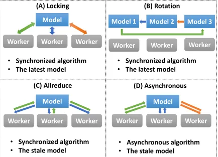
These attributes derive four types of computation models, each of which uses a different means

to handle the model and coordinate workers (see Figure 1). The computation model description

focuses on the distributed environment. However, computation models can also be applied to a

multi-thread environment. In a system with two levels of parallelism, model composition is

com-monly adapted, with one type of computation model at the distributed environment and another in

the multi-thread environment.

Computation Model A (Locking) This computation model uses a synchronized algorithm to coordinate parallel workers and guarantees each worker exclusive access to model parameters. Once

a worker trains a data item, it locks the related model parameters and prevents other workers from

accessing them. When the related model parameters are updated, the worker unlocks the parameters.

Thus the model parameters used in local computation is always the latest.

Computation Model B (Rotation) The next computation model also uses a synchronized algorithm. Each worker first takes a part of the shared model and performs training. Afterwards,

the model is shifted between workers. Through model rotation, each model parameters are updated

by one worker at a time so that the model is consistent.

Model

Worker

Worker

Worker

Model

Worker

Worker

Worker

Model

Worker

Worker

Worker

_Worker

_Worker

_Worker

Model 1

Model 2

Model 3

•

Synchronized algorithm

•

The latest model

•

Synchronized algorithm

•

The latest model

•

Synchronized algorithm

•

The stale model

•

Asynchronous algorithm

•

The stale model

(A) Locking

(B) Rotation

(C) Allreduce

(D) Asynchronous

required by local computation. When the local computation is completed, modifications of the local

model from all workers are gathered to update the model.

Computation Model D (Asynchronous) With this computation model, an asynchronous al-gorithm employs the stale model. Each worker independently fetches related model parameters,

performs local computation, and returns model modifications. Unlike the “Locking” computation

model, workers are allowed to fetch or update the same model parameters in parallel. In contrast to

‘Rotation” and “Allreduce”, there is no synchronization barrier.

Previous work shows many machine learning algorithms can be implemented in the MapReduce

programming model [6]; later on, these algorithms are improved by in-memory computation and

communication in iterative MapReduce [20, 21, 22]. However, the solution with broadcasting and

reducing model parameters is a special case of the “Allreduce” computation model and is not

im-mediately scalable as the model size grows larger than the capacity of the local memory. As models

may reach1010 ∼ 1012parameters, Parameter Server type solutions [23, 24, 25] store the model on a set of server machines and use the “Asynchronous” computation model. Petuum [19],

how-ever, uses a computation model mixed with both the “Allreduce” and “Asynchronous” computation

models [19]. Petuum also implements the “Rotation” computation model [26, 27, 28].

In practice, it is difficult to decide what algorithm and which computation model to use for the

parallelization solution of a machine learning application. Taking the LDA application as an

exam-ple, it can be solved by many different algorithms, such as CGS and Collapsed Variational Bayes

(CVB) [3]. If CGS is selected, then the SparseLDA algorithm [29] is the most common

imple-mentation. Then comes another question: which computation model should be used to parallelize a

machine learning algorithm? Currently there are various implementations (see Table 1). Potentially,

it is possible to have ways other than the implementations above to perform LDA CGS

paralleliza-tion, as long as the computation dependency is maintained. The difference between these solutions

is discussed in the section below.

2.3 Latent Dirichlet Allocation

Latent Dirichlet Allocation (LDA) is an important machine learning technique that has been widely

used in areas such as text mining, advertising, recommender systems, network analysis and genetics.

Table 1: The Computation Models of LDA CGS Implementations

Implementation Algorithm Computation Model

PLDA [30] CGS Allreduce

PowerGraph LDAa[31] CGS Allreduce

Yahoo! LDAb[24, 25] SparseLDA Asynchronous

Peacock [32] SparseLDA Asynchronous & Rotation

Parameter Server [23] CGS, etc. Asynchronous

Petuum Bosen [19] SparseLDA Asynchronous

Petuum Stradsc_{[26, 27, 28] SparseLDA Rotation & Asynchronous}

a _{https://github.com/dato-code/PowerGraph/tree/master/toolkits/topic_modeling} b _{https://github.com/sudar/Yahoo_LDA}

c _{https://github}

.com/petuum/bosen/wiki/Latent-Dirichlet-Allocation

to scale it to web-scale corpora to explore more subtle semantics with a big model which may

contain billions of model parameters [27]. The LDA application is commonly implemented by the

SparseLDA algorithm. In this section, the model synchronization patterns and the communication

strategies of this algorithm are studied. The size of model required for local computation is so

large that sending such data to every worker results in communication bottlenecks. The required

computation time is also great due to the large model size. However, the model size shrinks as

the model converges. As a result, a faster model synchronization method can speed up the model

convergence, in which the model size shrinks and reduces the iteration execution time.

For two well-known LDA implementations, Yahoo! LDA uses the “Asynchronous”

computa-tion model while Petuum LDA uses the “Rotacomputa-tion” computacomputa-tion model. Though using different

computation models, both solutions favor asynchronous communication methods, since it not only

avoids global waiting but also quickly makes the model update visible to other workers and thereby

boosts model convergence. However, my research shows that the model communication speed can

be improved with collective communication methods. With collective communication optimization,

the “Allreduce” computation model can outperform the “Asynchronous” computation model.

Be-sides, in the “Rotation” computation model, using collective communication can further reduce the

model communication overhead compared with using asynchronous communication.

2.3.1 LDA Background

LDA modeling techniques can find latent structures inside the training data which are abstracted as

z

_1,1

z

_i,j

z

_i,1

Document Collection

Topic assignment

x

_1,1

x

_i,j

x

_i,1

K*D

j

V*D

w

word-doc matrix

V*K

w

N

word-topic matrix

≈

×

j

M

topic-doc matrix

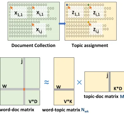
Figure 2: Topics Discovery

topics and each topic as a multinomial distribution over words. Then an inference algorithm works

iteratively until it outputs the converged topic assignments for the training data (see Figure 2).

Similar to Singular Value Decomposition, LDA can be viewed as a sparse matrix decomposition

technique on a word-document matrix, but it roots on a probabilistic foundation and has different

computation characteristics.

Among the inference algorithms for LDA, CGS shows high scalability in parallelization [32,

33], especially compared with another commonly used algorithm, CVB (used Mahout LDA5) .

CGS is a Markov chain Monte Carlo type algorithm. In the “initialize” phase, each training data

point, or token, is assigned to a random topic denoted aszij. Then it begins to reassign topics to

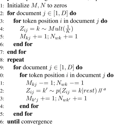
Table 2: LDA CGS Sequential Algorithm Pseudo Code Input: training dataX, the number of topicsK, hyperparametersα, β

Output: topic assignment matrixZ, topic-document matrixM, word-topic matrixN 1: InitializeM, N to zeros

2: fordocumentj∈[1, D]do

3: fortoken positioniin documentjdo 4: Zij =k∼M ult(_K1)

5: Mkj += 1;Nwk += 1 6: end for

7: end for 8: repeat

9: fordocumentj ∈[1, D]do

10: fortoken positioniin documentjdo

11: Mkj −= 1;Nwk −= 1

12: Zij =k0∼p(Zij =k|rest)//a 13: Mk0_j += 1;N_wk0 += 1

14: end for 15: end for

16: untilconvergence

a_{Sample a new topic according to Equation 5 using SparseLDA}

each tokenxij =wby sampling from a multinomial distribution of a conditional probability ofzij:

p zij =k|z¬ij, x, α, β∝ N

¬ij wk +β

P

wN ¬ij wk +V β

M_kj¬ij+α

(5)

Here superscript ¬ij means that the corresponding token is excluded. V is the vocabulary size.

Nwk is the token count of wordwassigned to topickinK topics, andMkj is the token count of topickassigned in documentj. The matricesZij,Nwk andMkj, are the model. Hyperparameters αandβ control the topic density in the final model output. The model gradually converges during

the process of iterative sampling. This is the phase where the “burn-in” stage occurs and finally

reaches the “stationary” stage.

The sampling performance is more memory-bound than CPU-bound. The computation itself

is simple, but it relies on accessing two large sparse model matrices in the memory. In Figure 2,

sampling occurs by the column order of the word-document matrix, called “sample by document”.

AlthoughMkjis cached when sampling all the tokens in a documentj, the memory access toNwk is random since tokens are from different words. Symmetrically, sampling can occur by the row

to the size of model matrices. SparseLDA is an optimized CGS sampling implementation mostly

used in state-of-the-art LDA trainers. In Line 10 of Table 2, the conditional probability is usually

computed for eachkwith a total ofKtimes, but SparseLDA decreases the time complexity to the

number of non-zero items in one row ofNwk and in one column ofMkj, both of which are much

smaller thanKon average.

2.3.2 Big Model Problem

Sampling onZij in CGS is a strict sequential procedure, although it can be parallelized without

much loss in accuracy [33]. Parallel LDA can be performed in a distributed environment or a

shared-memory environment. Due to the huge volume of training documents, the distributed environment is

required for parallel processing. In a distributed environment, a number of compute nodes deployed

with a single worker process apiece. Every worker takes a partition of the training document set and

performs the sampling procedure with multiple threads.

The LDA model contains four parts: I.Zij - topic assignments on tokens, II.Nwk- token counts of words on topics (word-topic matrix), III. Mkj - token counts of documents on topics (topic-document matrix), and IV.P

wNwk- token counts of topics. HereZij is always stored along with the training tokens. For the other three, because the training tokens are partitioned by document,

Mkj is stored locally whileNwk andP

wNwk are shared. For the shared model parts, a parallel LDA implementation may use the latest model or the stale model in the sampling procedure.

Now it is time to calculate the size ofNwk, a huge but sparseV ×K matrix. The word

distri-bution in the training data generally follows a power law. If the words based on their frequencies is

sorted from high to low, for a word with ranki, its frequency isf req(i) =C·i−λ. Then forW,

the total number of training tokens, there is

W = V

X

i=1

f req(i) = V

X

i=1

(C·i−λ)≈C·(lnV +γ+ 1

2V) (6)

To simplify the analysis,λis considered as1. SinceCis a constant equal tof req(1), thenW is the

partial sum of the harmonic series which have logarithmic growth, whereγis the Euler-Mascheroni

constant≈0.57721. The real model sizeSdepends on the count of non-zero cells. In the “initialize”

100 ₁₀1 ₁₀2 ₁₀3 ₁₀4 ₁₀5 ₁₀6 ₁₀7

Word Rank

Word Frequency

y

_x

enwiki

y

_x

100 ₁₀1 ₁₀2 ₁₀3 ₁₀4

Document Collection Partition Number

Vocabulary Size of Partition (%)

clueweb

enwiki

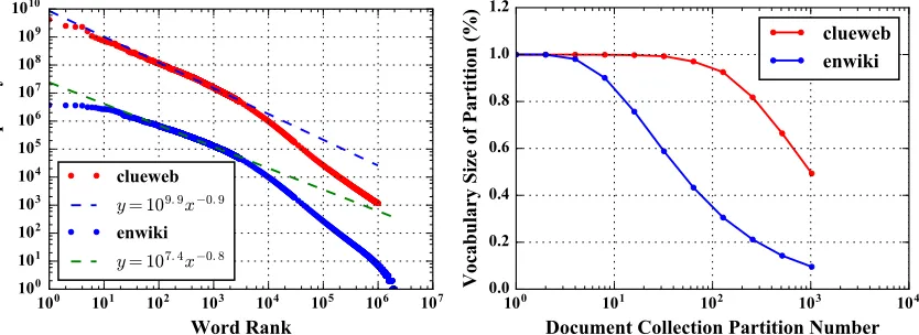
(a) Zipf’s Law of the Word Frequencies (b) Vocabulary Size vs. Document Partitioning

Figure 3: Words’ Distribution on the Training Documents

f req(J) =K, thenJ =C/K, and there is:

Sinit= J X i=1 K+ V X

i=J+1

f req(i) =W−

J

X

i=1

f req(i) + J

X

i=1

K =C·(lnV +lnK−lnC+ 1) (7)

The initial model sizeSinitis logarithmic to matrix sizeV ·K, which meansS << V K. However

this does not meanSinit is small. Since C can be very large, evenC ·ln(V K) can result in a

large number. In the progress of iterations, the model size shrinks as the model converges. When a

stationary state is reached, the average number of topics per word drops to a certain small constant

ratio ofK, which is determined by the concentration parametersα,βand the nature of the training

data itself.

The local vocabulary size V0 on each worker determines the model volume required for local

computation. When documents are randomly partitioned toN processes, every word with a

fre-quency higher than N has a high probability of occurring on all the processes. Iff req(L) = N

at rank L, thenL = _(lnVW_+γ)·N. For a large training dataset, the ratio betweenL andV is often very high, indicating that local computation requires most of the model parameters. Figure 3 shows

the difficulty of controlling local vocabulary size in random document partitioning. When 10 times

more partitions are introduced, there is only a sub-linear decrease in the vocabulary size per

parti-tion. The “clueweb” and “enwiki” datasets are used as examples (see Section 2.3.5). In “clueweb”,

each partition gets 92.5% ofV when the training documents are randomly split into 128 partitions.

Model

Worker

Worker

Worker

•

A1. PLDA

- Optimized collective

A2. PowerGraph LDA

- Unoptimized collective

A3. Yahoo! LDA

- Point-to-point

B. Rotation

A. Allreduce/Asynchronous

Worker

Worker

Worker

Model 1

Model 2

Model 3

•

B1. Petuum LDA

_{- Point-to-point}

Figure 4: Synchronization Methods under Different Computation Models

a similar ratio. In summary, though the local model size reduces as the number of compute nodes

grows, it is still a high percentage ofV in many situations.

In conclusion, there are three key properties of the LDA model:

1. The initial model size is huge but it reduces as the model converges

2. The model parameters required in local computation is a high percentage of all the model

parameters

3. The local computation time is related to the local model size

These properties indicate that the communication optimization in model synchronization is

neces-sary because it can accelerate the model update process and result in a huge benefit in computation

and communication of later iterations.

Of the various synchronization methods used in state-of-the-art implementations, they can be

categorized into two types (see Figure 4). In the first type, the parallelization either uses the

work on stale model parameters. In PLDA, without storing a shared model, it synchronizes local

model parameters through a MPI “allreduce” operation [34]. This operation is routing optimized,

but it does not consider the model requirement in local computation, causing high memory usage and

high communication load. In PowerGraph LDA, model parameters are fetched and returned directly

in a synchronized way. Though it communicates less model parameters compared with PLDA, the

performance is low for lack of routing optimization. Unlike the two implementations above which

use the “Allreduce” computation model, a more popular implementation, Yahoo! LDA, follows

the “Asynchronous” computation model. Yahoo! LDA can ease the communication overhead with

asynchronous point-to-point communication, however, its model update rate is not guaranteed. A

word’s model parameters may be updated either by changes from all the training tokens, a part of

them, or even no change. A solution to this problem is to combine the “Allreduce” computation

model and the “Asynchronous” computation model. This is implemented in Petuum Bosen LDA

[19]. In the second type, the “Rotation” computation model is used. Currently only Petuum Strads

LDA is in this category. In its implementation, parameters are sent to the neighbor asynchronously.

A better solution for the first type of synchronization method can be a conjunction of PLDA and

PowerGraph LDA with new collective communication optimizations which include both routing

optimization and reduced data size for communication. There are three advantages to such a

strat-egy. First, considering the model requirement in local computation, it reduces the model parameters

communicated. Second, it optimizes routing through searching “one-to-all” communication

pat-terns. Finally, it maintains the model update rate compared with the asynchronous method. For the

second type of synchronization method, using collective communication is also helpful because it

maximizes bandwidth usage between compute nodes and avoids flooding the network with small

messages, which is what Petuum Strads LDA does.

2.3.3 Model Synchronization Optimizations

New solutions with optimized collective communication operations to parallelize the SparseLDA

algorithm are developed. Model parameters are distributed among workers. Two model

synchro-nization methods are used. In the first method, a set of local models are defined on each worker.

Each local model is considered a local version of the global model. The synchronization has two

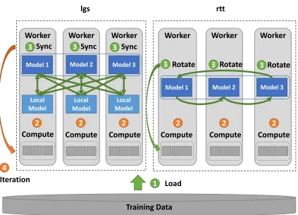
Training Data

1

Worker

Worker

Worker

Compute

3

Sync

Figure 5: LDA implementations with Optimized Communication

global model to local models. The second step reduces the updates from different local models to

one in the global model. Model parameters are packed into chunks and sent to avoid small message

flooding. Routing optimized broadcasting [34] is used if “one-to-all” communication patterns are

detected on a set of model parameters. In the second method, “rotate” considers processes in a ring

topology and shifts the model chunks from one process to the next neighbor. The model parameters

are partitioned based on the range of word frequencies in the training dataset. The lower the

fre-quency of the word, the higher the word ID given. Then the word IDs are mapped to process IDs

based on the modulo operation. In this way, each process contains model parameters with words

whose frequencies are ranked from high to low. In the first synchronization method, this kind of

model partitioning can balance the communication load. In the second synchronization method, it

can balance the computation load on different workers between two times of model shifting.

As a result, two parallel LDA implementations are presented (see Figure 5). One is “lgs” (an

Table 3: Training Data and Model Settings in the Experiments

Dataset Number Number Vocabulary Doc Length Number Initial

of Docs of Tokens Mean/SD of Topics Model Size

clueweb 50.5M 12.4B 1M 224/352 10K 14.7GB

enwiki 3.8M 1.1B 1M 293/523 10K 2.0GB

bi-gram 3.9M 1.7B 20M 434/776 500 5.9GB

In both implementations, the computation and communication are pipelined to reduce the

synchro-nization overhead, i.e., the model parameters are sliced in two and communicated in turns. Model

Part IV is synchronized through an “allreduce” operation at the end of every iteration. In the local

computation, both “lgs” and “rtt” use the “Asynchronous” computation model. However, “lgs”

sam-ples by document while “rtt” samsam-ples by word. All these are done to keep the consistency between

implementations for unbiased communication performance comparisons in experiments. Of course,

for “rtt”, since each model shifting only gives a part of model parameters for the local computation,

sampling by word can easily reduce the time used for searching tokens which can be sampled.

2.3.4 Experiments

Experiments are done on an Intel Haswell cluster. This cluster contains 32 nodes each with two

18-core 36-thread Xeon E5-2699 processors and 96 nodes each with two 12-core 24-thread Xeon

E5-2670 processors. All the nodes have 128GB memory and are connected with 1Gbps Ethernet

(eth) and Infiniband (ib). For testing, 31 nodes with Xeon 2699 and 69 nodes with Xeon

E5-2670 are used to form a cluster of 100 nodes, each with 40 threads. All the tests are done with

Infiniband through IPoIB support.

“clueweb”6, “enwiki”, and “bi-gram”7are three datasets used (see Table 3). The model settings

are comparable to other research work [27], each with a total of 10 billion parameters. α andβ

are both fixed to a commonly used value 0.01 to exclude dynamic tuning. Several implementations

are tested: “lgs”, “lgs-4s” (“lgs” with 4 rounds of model synchronization per iteration, each round

with 1/4 of the training tokens), and “rtt”. To evaluate the quality of the model outputs, the model

likelihood on the words’ model parameters is used to monitor model convergence. These LDA

im-plementations are compared with Yahoo! LDA and Petuum LDA, and thereby how communication

6_{10% of ClueWeb09, a collection of English web pages, http://lemurproject.org/clueweb09.php/} 7

0 50 100 150 200

Iteration Number

Model Likelihood

lgs

Yahoo!LDA

rtt

Petuum

lgs-4s

0 50 100 150 200

Iteration Number

Model Likelihood

lgs

Yahoo!LDA

rtt

Petuum

(a) Model Convergence Speed on “clueweb” (b) Model Convergence Speed on “enwiki”

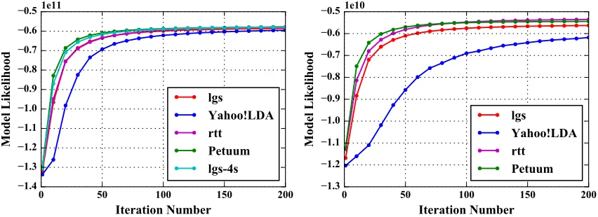
Figure 6: Model Convergence Speed by Iteration Count

methods affect LDA performance are learned by studying the model convergence speed.

The model convergence speed is firstly measured by analyzing model outputs on Iteration 1,

10, 20... 200. In an iteration, every training token is sampled once. Thus the number of model

updates in each iteration is equal. Then how the model converges with the same amount of model

updates is measured. On “clueweb” (see Figure 6(a)), Petuum has the highest model likelihood on

all the iterations. Due to “rtt”’s preference of using stale thread-local model parameters in

multi-thread sampling, the convergence speed is slower. The lines of “rtt” and “lgs” are overlapped for

their similar convergence speeds. In contrast to “lgs”, the convergence speed of “lgs-4s” is as high

as Petuum. This shows that increasing the number of model update rounds improves convergence

speed. Yahoo! LDA has the slowest convergence speed because asynchronous communication

does not guarantee all model updates are seen in each iteration. On “enwiki” (see Figure 6(b)), as

before, Petuum achieves the highest accuracy out of all iterations. “rtt” converges to the same model

likelihood level as Petuum at iteration 200. “lgs” demonstrates slower convergence speed but still

achieves high model likelihood, while Yahoo! LDA has both the slowest convergence speed and

the lowest model likelihood at iteration 200. Though the number of model updates is the same, an

implementation using the stale model converges slower than one using the latest model. For those

using the stale model, “lgs-4s” is faster than “lgs” while “lgs” is faster than Yahoo! LDA. This

means by increasing the number of model synchronization rounds, the model parameters used in

computation are newer, and the convergence speed is improved.

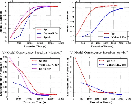
speed between “lgs” and Yahoo! LDA is compared. On “clueweb”, the convergence speed is shown

based on the elapsed execution time (see Figure 7(a)). Yahoo! LDA takes more time to finish

Itera-tion 1 due to its slow model initializaItera-tion, which demonstrates that it has a sizable overhead on the

communication end. In later iterations, while “lgs” converges faster, Yahoo! LDA catches up after

30 iterations. This observation can be explained by the slower computation speed of the current

Java implementation. To counteract the computation overhead, the number of model

synchroniza-tion rounds per iterasynchroniza-tion is increased to four. Thus the computasynchroniza-tion overhead is reduced by using

a newer and smaller model. Although the execution time of “lgs-4s” is still slightly longer than

Yahoo! LDA, it obtains higher model likelihood and maintains faster convergence speed during the

whole execution. Similar results are shown on “enwiki”, but this time “lgs” not only achieves higher

model likelihood but also has faster model convergence speed throughout the whole execution (see

Figure 7(b)). From both experiments, it is learned that though the computation is slow in “lgs”, with

collective communication optimization, the model size quickly shrinks so that its computation time

is reduced significantly. At the same time, although Yahoo! LDA does not have any extra overhead

other than computation in each iteration, its iteration execution time reduces slowly because it keeps

computing with an older model (see Figure 7(c)(d)).

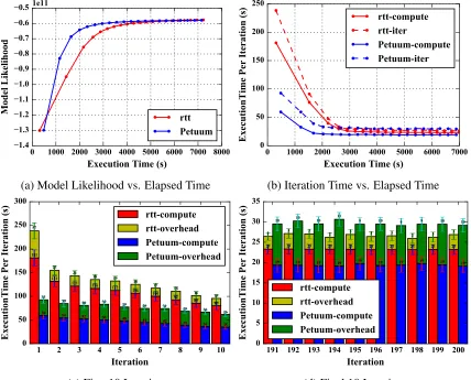
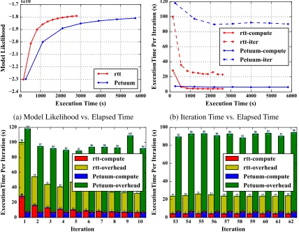
Next “rtt” and Petuum LDA are compared on “clueweb”and “bi-gram”. On “clueweb”, the

ex-ecution times and model likelihood achieved on both sides are similar (see Figure 8(a)). Both are

around 2.7 times faster than the results in “lgs” and Yahoo! LDA. This is because they use the

lat-est model parameters for sampling, which quickly reduces the model size for further computation.

Besides, sampling by word leads to better local computation performance compared with

sam-pling by document due to less model parameter fetching/updating conflict in the “Asynchronous”

computation model. Though “rtt” has higher computation time compared with Petuum LDA, the

communication overhead per iteration is lower. When the execution arrives at the final few

itera-tions, while computation time per iteration in “rtt” is higher, the whole execution time per iteration

becomes lower (see Figure 8(b)(c)(d)). This is because Petuum communicates each word’s model

parameters in small messages and generates high overhead. On “bi-gram”, the results show that

Petuum does not perform well when the number of words in the model increases. The high

over-head in communication causes the convergence speed to be slow, and Petuum cannot even continue

0 5000 10000 15000 20000 25000

Execution Time (s)

1.4 1.3 1.2 1.1 1.0 0.9 0.8 0.7 0.6 0.5

Model Likelihood

lgs

Yahoo!LDA

lgs-4s

0 500 1000 1500 2000 2500 3000 3500

Execution Time (s)

1.3 1.2 1.1 1.0 0.9 0.8 0.7 0.6 0.5

Model Likelihood

lgs

Yahoo!LDA

(a) Model Convergence Speed on “clueweb” (b) Model Convergence Speed on “enwiki”

0 5000 10000 15000 20000 25000

Execution Time (s)

0 100 200 300 400 500 600 700 800

ExecutionTime Per Iteration (s)

lgs-iter

Yahoo!LDA-iter

lgs-4s-iter

0 500 1000 1500 2000 2500 3000 3500

Execution Time (s)

0 10 20 30 40 50 60 70 80

ExecutionTime Per Iteration (s)

lgs-iter

Yahoo!LDA-iter

(c) Per Iteration Time on “clueweb” (d) Per Iteration Time on “enwiki”

0 1000 2000 3000 4000 5000 6000 7000 8000

Execution Time (s)

1.4 1.3 1.2 1.1 1.0 0.9 0.8 0.7 0.6 0.5

Model Likelihood

rtt

Petuum

0 1000 2000 3000 4000 5000 6000 7000

Execution Time (s)

0 50 100 150 200 250

ExecutionTime Per Iteration (s)

rtt-compute

rtt-iter

Petuum-compute

Petuum-iter

(a) Model Likelihood vs. Elapsed Time (b) Iteration Time vs. Elapsed Time

1 2 3 4 5 6 7 8 9 10

Iteration

ExecutionTime Per Iteration (s)

181 131 121 ₁₁₆ 112 ₁₀₆ 100 92 85 ₈₀ 57 23 21 18 19 18 17 ₁₈ 16 ₁₅

59 _{54 52}

50 48 44 42 39 36 35

33

30 ₂₈ 32 ₂₉

29 31 ₂₉

30 ₂₆

rtt-compute

rtt-overhead

Petuum-compute

Petuum-overhead

191 192 193 194 195 196 197 198 199 200

Iteration

ExecutionTime Per Iteration (s)

23 23 23 23 23 23 23 23 23 23

3 3 3 2 3 3 3 ₂ 3 3

19 19 19 19 19 19 19 19 19 19

10 10 10 11 9 10 9 9 10 10

rtt-compute

rtt-overhead

Petuum-compute

Petuum-overhead

(c) First 10 Iteration (d) Final 10 Iteration

0 1000 2000 3000 4000 5000 6000

Execution Time (s)

2.4 2.3 2.2 2.1 2.0 1.9 1.8 1.7

Model Likelihood

rtt

Petuum

0 1000 2000 3000 4000 5000 6000

Execution Time (s)

0 20 40 60 80 100 120

ExecutionTime Per Iteration (s)

rtt-compute

rtt-iter

Petuum-compute

Petuum-iter

(a) Model Likelihood vs. Elapsed Time (b) Iteration Time vs. Elapsed Time

1 2 3 4 5 6 7 8 9 10

Iteration

ExecutionTime Per Iteration (s)

28

16

12 ₁₁

10 9 8 7 7 6

71 38 31 29 36 36 27 ₂₅ 25 25

7 7 7 7 6 6 6 6 6 6

110

87

84 ₈₂

81

86 86 85

102 84

rtt-compute

rtt-overhead

Petuum-compute

Petuum-overhead

53 54 55 56 57 58 59 60 61 62

Iteration

ExecutionTime Per Iteration (s)

19 20 21 21 _{19 19 19 19 19} 20

6 6 6 6 6 6 6 6 6 6

82 86 86 84 86 81

86 87 83 88

rtt-compute

rtt-overhead

Petuum-compute

Petuum-overhead

(c) First 10 Iteration (d) Final 10 Iteration

In sum, the model properties in parallel LDA computation suggest that using collective

commu-nication optimizations can improve the model update speed, which allows the model to converge

faster. When the model converges quickly, its size shrinks greatly, and the iteration execution time

also reduces. Optimized collective communication methods is observed to perform better than

asynchronous methods. “lgs” results in faster model convergence and higher model likelihood at

iteration 200 compared to Yahoo! LDA. On “bi-gram”, “rtt” shows significantly lower

communi-cation overhead than Petuum Strads LDA, and the total execution time of “rtt” is 3.9 times faster.

On “clueweb”, although the computation speed of the first iteration is 2- to 3-fold slower, the total

execution time remains similar.

Despite the implementation differences between “rtt”, “lgs”, Yahoo! LDA, and Petuum LDA,

the advantages of collective communication methods are evident. Compared with asynchronous

communication methods, collective communication methods can optimize routing between

paral-lel workers and maximize bandwidth utilization. Though collective communication will result in

global waiting, the resulting overhead is not as high as speculated when the load-balance is handled.

The chain reaction set off by improving the LDA model update speed amplifies the benefits of using

collective communication methods. When putting all the performance results together, it is also

clear that both “rtt” and Petuum are remarkably faster than the rest implementations. This shows

in LDA parallelization, using the “Rotation” computation model can achieve higher performance

compared with the “Allreduce” and “Asynchronous” computation model. Between the “Allreduce”

and “Asynchronous” two computation models, “lgs” proves to be faster than Yahoo! LDA at the

beginning, but at later stages, their model convergence speed tends to overlap. Through adjusting

the number of model synchronization frequencies to 4 per iteration, “lgs-4s” exceeds Yahoo! LDA

from start to finish. This means with the optimized collective communication, the “Allreduce”

com-putation model can exceed the “Asynchronous” comcom-putation model. From these results, it can be

concluded that the selection of computation models, combined with the details of computation

load-balancing and communication optimization, needs to be carefully considered in the implementation

3 Solving Big Data Problem with HPC Methods

The LDA application presents an example which shows selecting a proper computation model is

important to the machine learning algorithm parallelization and using collective communication

op-timization can improve the model synchronization speed. However, existing tools for parallelization

have limited support to the computation models and collective communication techniques. Since

the collective communication has been commonly used in the HPC domain, it is a chance to adapt

it to big data machine learning and derive an innovative solution.

3.1 Related Work

Before the emergence of big data tools, MPI is the primary tool used for parallelization in the HPC

domain. Other than “send” and “receive” calls, MPI provides collective communication

opera-tions such as “broadcast”, “reduce”, “allgather” and “allreduce”. These operaopera-tions provide efficient

communication performance through optimized routing. However, these operations only describe

the relations between parallel processes in the collective communication, when fine-grained model

synchronization is required, these collective communication operations lacks of a mechanism to

identify the relations between model updates and parameters in the synchronization. In this case,

lots of “send” and “receive” calls are used, which makes the application code complicated.

Different from MPI, big data tools focus on the synchronization based on the relations between

data items. In MapReduce [5], input data are read as Key-Value pairs and in the “shuffle” phase,

intermediate data are regrouped based on keys. So the communication pattern between processes

depends on the distribution of the intermediate data. Initially, MapReduce proved very successful as

a general tool to process many problems but was later considered not optimized for many important

analytics, especially those machine learning algorithms involving iterations. The reason is that the

MapReduce frameworks have to repeat loading training data from distributed file systems (HDFS)

each iteration. Iterative MapReduce frameworks such as Twister [7] and Spark [8] improve the

performance through caching invariable training data. To solve graph problems, Pregel [9], Giraph8,

and GraphLab [31, 35] abstract the training data as a graph, cache, and process it in iterations.

The synchronization is performed as message passing along the edges between neighbor vertices.

8

Though the synchronization relations between data items/model parameters are expressed in these

tools, there are still limitations. In MapReduce, the dependency between model parameters and

local training data is not well solved, so that model parameters are only broadcasted to the workers

or reduced to one in the execution flow, making the implementation hard to scale. This is seen in the

K-means Clustering implementations of Mahout on Hadoop9or Spark MLlib10. Other applications’

complicated synchronization dependency also require multiple ways of model synchronization (e.g.

the SparseLDA algorithm). However, both MapReduce and Graph tools follow the “Allreduce”

computation model, it is impossible for developers to parallelize SparseLDA with the “Rotation”

computation model within these frameworks.

Routing optimization is another important feature which is missing in existing big data tools.

For example, in K-Means with Lloyd’s algorithm [12], the training data (high dimensional points)

can be easily split and distributed to all the workers, but the model (centroids) have to be

synchro-nized and redistributed to all the parallel workers in the successive iterations. Mahout on Hadoop

chooses to reduce model updates from all the map tasks in one Reduce task, generate the new model,

store it on HDFS, and let all the Map tasks read the model back to memory. The whole process can

be summarized as “reduce-broadcast”. According to C.-T. Chu et al. [6], this pattern can be applied

to many other machine learning algorithms, including Logistic Regression, Neural Networks,

Prin-cipal Component Analysis, Expectation Maximization and Support Vector Machines, all of which

follow the statistical query model. However, when both the size of the model and the number of

workers grow large, this method becomes inefficient. In K-Means Clustering, the time

complex-ity of this communication process isO(pkd), where pis the number of workers, kis the number

of centroids, anddis the number of dimensions per centroid/point. In my initial research work,

a large-scale K-Means clustering on Twister is studied. Image features from a large collection of

seven million social images, each representing as a point in a high dimensional vector space, are

clustered into one million clusters [20, 21]. This clustering application is split into five stages in

each iteration: “broadcast”, “map”, “shuffle”, “reduce”, and “combine”. By applying a three-stage

synchronization of “regroup-gather-broadcast” with, the overhead of data synchronization can be

reduced toO(3kd). Furthermore, if “regroup-allgather” is applied directly, the communication time

9

https://mahout.apache.org

10 _{https://spark}

Table 4: Programming Models and Synchronization Patterns of Big Data Tools

Tool Programming Model Synchronization Pattern

MPI

a set of parallel workers are spawned with com-munication support be-tween them

send/receive or collective communication opera-tions

Hadoop

(iterative) MapReduce, DAG-like job execution flow may be supported

disk-based shuffle between the Map stage and the Reduce stage

Twister in-memory regroup between the Map stage and

the Reduce stage; “broadcast” and “aggregate”

Spark RDD transformations on RDD; “broadcast” and

“aggregate”

Giraph

BSP model, data are expressed as vertices and edges in a graph

graph-based message communication following the Pregel model (vertex-based partitioning, messages are sent between neighbor vertices)

Hama

graph-based communication following the Pregel model or direct message communication between workers.

GraphLab (Turi)

graph-based communication through caching and fetching of ghost vertices and edges, or the com-munication between a master vertex and its repli-cas in the PowerGraph (GAS) model

GraphX graph-based communication supports both Pregel

model and PowerGraph model

Parameter

Server BSP model, or loosely synchronized on the parameter server

asynchronous “push” and “pull” calls are used for communicating model parameters between pa-rameter servers and workers

Petuum

in addition to asynchronous “push” and “pull” calls, the framework allows scheduling model pa-rameters between workers

can even be reduced toO(2kd). The LDA application is another example to show the advantages

of collective communication with routing optimization, as what has been discussed in the previous

section. Both Parameter Server-type Yahoo! LDA and Petuum are inefficient in communication due

to asynchronous parameter-based point-to-point communication.

In sum, existing tools can be listed with their programming models and synchronization

pat-terns (see Table 4). The first one is MPI. It spawns a set of parallel processes and perform

syn-chronization through “send”/“receive” calls or collective communication operations based on the

process relations. Next is the MapReduce type, MapReduce systems such as Hadoop describes the

parallelization as processing inputs as Key-Value pairs in the Map tasks, generating intermediate

yet is still slow when running iterative algorithms. Frameworks like Twister, Spark, and HaLoop

[36] solved this issue by caching the training data and extend MapReduce to iterative MapReduce.

In Spark, multiple MapReduce jobs can form a directed acyclic execution graph with additional

work flow management to support complicated data processing. The third type is the graph

process-ing tools, which abstracts data as vertices and edges and executes in the BSP (Bulk Synchronous

Parallel) model. Pregel and its open source version Giraph and Hama11 follow this design. By

contrast, GraphLab [35] abstracts data as a graph but uses consistency models to control vertex

value updates (no explicit message communication calls). GraphLab (now called Turi12) was later

enhanced with PowerGraph [31] abstractions to reduce the communication overhead. This was also

used by GraphX [37]. The fourth type of tools directly serve machine learning algorithms through

providing programming models for model parameter synchronization. These tools include

Param-eter Server and Petuum. ParamParam-eter Server does not force global synchronization. ParamParam-eters are

stored in a separate group of servers. Parallel workers can exchange model updates with servers

asynchronously. In addition to the model synchronization between workers and servers, Petuum

also allows to schedule and shift model parameters between workers.

3.2 Research Methodologies

Based on the requirements of model synchronization in parallel machine learning algorithms, and

the discussion about the status quo of how the computation models and collective communication

techniques are applied in existing tools, it is necessary to build a separate communication layer with

high level programming interfaces to provide a rich set of communication operations, granting users

flexibility and easiness to develop machine learning applications. There are three challenges derived

from prior research:

Express Communication Patterns from Different Tools From the four computation models, the “Allreduce” and “Rotation” computation models can be expressed with collective

communi-cation operations. As what is shown in the related work, each tool has its own synchronization

operations, either based on the process relations or the data item relations. For a unified

collec-tive communication layer, it is necessary to unite different synchronization patterns into one layer

11

https://hama.apache.org

12