A finite element solution of thermal wave propagation in elastic media

Theses

Thesis/Dissertation Collections

4-1-1987

A finite element solution of thermal wave

propagation in elastic media

Dominic N. Dalo

Follow this and additional works at:

http://scholarworks.rit.edu/theses

This Thesis is brought to you for free and open access by the Thesis/Dissertation Collections at RIT Scholar Works. It has been accepted for inclusion

in Theses by an authorized administrator of RIT Scholar Works. For more information, please contact

ritscholarworks@rit.edu

.

Recommended Citation

by

Dominic N. Dalo

A Tbesis Submitted

in

Partial Fulfillment

of the

Requirements

for the Degree of

MASTER OF SCIENCE

in

Mechanical

Engineering

(Thesis Advisor)

Prof.

----.".,.=,...-==,----

_

Approved by:

Prof.

_

Prof.

_

<Department Head)

Prof.

---"====,..,,,=;,-

_

DEPARTMENT OF MECHANICAL ENGINEERING

COLLEGE OF ENGINEERING

ROCHESTER INSTITUTE OF TECHNOLOGY

ROCHESTER, NEW YORK

I Dominic N.

Palo

hereby

grantpermission

to the

Wallace

Memorial

Library,

of

R.I.T.,

to

reproduce

my thesis in

wholeor

in

part.

Any

reproduction will not

be

for

commercialuseor profit.

3 April 1987

To

my

Mother

and

Father,

who

have

provided

the

support and encouragement

to

allow me

to

achieve, I

dedicate

this

work.

To Dr.

Hany Ghoneim,

my thesis

advisor,

I

wish

to

express

my

deepest

gratitude and

bestow

the

accolade of

being

the

professor who

has

most

stimulated

my

desire

to

learn.

To

Drs.

William

F. Halbleib

and

Robert A.

Ellson,

who

taught

me

the

fundamentals

ofmechanics and

thermodynamics,

my thanks

andadmiration.

To Drs.

Charles

W. Haines

and

Bhalchandra V.

Karlekar,

my

appreciation

for

providing

mewith

invaluable

guidance

during

my

college career.

And

finally

to

the

membersof

my thesis

defense

committee,

I

am much obliged

for

the time

they

spent

reading

and

evaluating my

work.

The

rational

theory

of

thermodynamics

is

used

to

develop

equations

governing the

propagation of

thermal

waves.

A

new vector

quantity

is

introduced

to

account

for

the

thermal

waves.

The

phenomenon of

thermal

wave

propagation

is

illustrated

by

considering the

problem of one-dimensional

heat

conduction

in

a

finite

slab subjected

to

a

heat flux

pulse.

The

solution

is

obtained via

the

finite

element method.

A

discussion

of

the

results and

their

significance

is

also presented.

List

of

Figures

vi

Nomenclature

vii

1.0

INTRODUCTION

1

1.1

Historical Review

1

1.2

Literature Review

1

1.3

Approach

Taken

3

1.4

Notation

3

2.0

THEORY

5

2.1

List

of

Fundamental

Quantities

5

2.2

Fundamental Equations

of

Continuum Mechanics

6

2.3

Constitutive

Relations

7

2.4

Derivation

of

Equations

8

3.0

PROBLEM DESCRIPTION

13

3.1

Definition

of

Problem

13

3.2

Dimensional

Analysis

15

4.0

FINITE ELEMENT IMPLEMENTATION

17

4.1

Function

Approximation

17

4.2

Weighted Residual

19

4.3

Temporal Approximation

22

5.0

RESULTS

AND DISCUSSION

25

5.1

Temperature

Response

25

5.2

Thermal

Flux

27

5.3

Thermal

Waves

27

5.4

Finite

Element

Program

36

6.0

CONCLUSIONS

39

References

41

Appendices

A.

Formation

of

Finite Element Matrices

43

Figure

Caption

Page

1

Geometry

and

Thermal

Conditions

14

2

Shape Functions

for

Linear

Elements

18

3

Thermal Response for Various Values

of

Alpha

26

4

Heat Flux Profiles for

a =

10.0,

x =

0.15

28

5

Heat

Flux

Profiles for

a =

100.0,

x =

0.05

29

6

Heat Flux

Profiles

for

a =

1000.0,

_x =

0.025

30

7

Temperature Profiles for

a =

10.0

31

8

Temperature Profiles for

a =

100.0

32

9

Temperature Profiles for

a =

1000.0

33

10

Temperature Profiles for

a =

1000.0

after reflection of

thermal

wave

35

A

materialconstant associatedwithelastic

heat flux

a

dimensionless

_{material parameter}

b

dimensionless

elastic

heat

flux

Cv

specific

heat

at constant volume

e specific

internal

energy

6

weighting

parameter

k

thermal

diffusivity

k

thermal

conductivity

h

length

of

finite

element

p

mass

density

r

internal

heat

supply

perunit mass

s specific

entropy

x

dimensionless

time

t

time

T

temperature

u

dimensionless

temperature

ti/

Helmholtz

free

energy

co

frequency

of

heat

pulse

X

dimensionless

position

x position

Qo

amplitudeof

heat

pulse

First Order Tensors

Pi

elastic

heat

flux

bi

dimensionless

elastic

heat

flux

fi

body

force

perunit mass

gi

constitutive relation associatedwithelastic

heat flux

qi

total

heat

flux

perunit area

4>i

shape

function

associatedwith

b

Bi

nodalvaluesof

dimensionless

elastic

heat flux

U,

nodalvaluesof

dimensionless

temperature

Higher

Order Tensors

Yij

coefficient of

thermal

expansion

tensor

eij

total

strain

tensor

eejj

elastic strain

tensor

oij

total

stress

tensor

kjj

thermal conductivity

tensor

Dijkl

elastic modulus

tensor

1.1

HISTORICAL

BACKGROUND

The

conduction of

heat

in

materials

has

long

been

established as a

diffusion

process

that

is

directly

proportional

to the

temperature

gradient anda

material

property

defined

as

the

thermal

conductivity.

A

seriesof

experiments,

the

first

of which wasconducted

in

the

mid-1940's

have indicated

that thermal

disturbances

can propagate as waves.

Peshkov

[1],

the

earliest of

the

investigators

to

observe

these

thermal waves,

introduced

the term

"second

sound"

to

describe

the

waves'

analogous

behavior

to

ordinary

sound waves.

Peshkov's

experimentswere conducted

using

liquid helium

ata

temperature

of

approximately 2

K.

Nearly

twenty

years

later,

Ackerman

and

his

associates

[2]

were able

to

repeat

Peshov's

findings

using

solid

helium

crystals,

again at cryogenic

temperatures.

Similar

experiments

have

been

conducted

using

halogen

alkalicrystalswith no

definitive

results.

Hence,

to

date,

second sound

effects

have

only been

observed

in

non-metallic materials and under

very

special conditions.

1.2

LITERATURE

REVIEW

Due

to

the

nature of

the

materials and conditions

in

which

the

second

soundwaves

have

been

observed,

modern physicists

believe

that

thermal

wave

propagation

is

a microscopic phenomenon

that

falls

into

the

realm ofquantum

mechanics.

Bertman

and

Sandiford

[3]

give a

non-mathematical,

but

otherwise

materials,

such as

liquid

and solid

helium

which

have had

all

impurities

"frozen

out"

of

them,

are

thought to

promote

the

propagation of

these

phonons.

Impure

or "dirty"

materials,

which

includes

all

metals,

contain so

many

imperfections

that the

phonons are scattered

in

a random

fashion

resulting in

classical

heat diffusion.

In

keeping

with quantum

theory,

second sound effects

are proposed

to

occur

only

at

discrete

energy

levels

i.e.,

only

phononsofspecific

frequencies

canpropagate as a wave.

There

are

those

of another

school,

mainly

classical

physicists,

mathematicians and

engineers,

who

believe

that

thermal

wave propagation can

be

explained

using

a continuum approach.

Lord

and

Shulman

[4]

were

among the

earliest researchers

known

to

present a generalized

theory

of

thermoelasticity

which accounted

for

the

propagation of

thermal

waves.

Their

approach

is based

upon

modifying the

classical

Fourier

law

of

heat

conduction

to

include

an additional

term

which

involves

the

rateofchange of

the

heat

flux.

This

modification

generally

results

in

a

hyperbolic

heat

conduction equation as

opposed

to

the

standard parabolic

form.

Ozisik

and

Vick

[5]

present a closed

form

solution

to

an uncoupled one-dimensional

hyperbolic heat

conduction

equation.

Their

results

indicate

that

this

type

of modification

to

the

law

of

heat

conduction

does

result

in

asolution

that

exhibits

oscillatory

behavior.

Researchers have

sought

to

develop

theories

which validate

the

modificationof

the

Fourier's law in

this

manner.

Others have

taken

different

approaches

to

the

development

of

the

equations

governing the

propagation of

thermal

waves.

Bogy

and

Naghdi

[6]

show

how

equations

may

be

obtained

by

statementof

the

second

law

of

thermodynamics

as

the

basis

of

their

theory.

A

vector

field

is

introduced

to

represent

the

flow

of a microscopic excitation

thought

to

originate

the

thermal

waves

in

the

work of

Atkin

and

his

associates

[9]. While

someof

preceding

works

have

obtainedpossible

field

equations,

none

have

presented

any

quantitative results

for

comparative purposes.

1.3

APPROACH TAKEN

In this

work,

the

rational

theory

of

thermodynamics

was employed

to

develop

coupled

thermoelastic

field

equations which account

for

the

thermal

waves.

An

additional constitutive relation was

introduced

to

define

a new vector

quantity

associated with

the

second sound waves.

The

ensuing

partial

differential

equations

along

with

the

fundamental

equations of continuum

mechanics are sufficient

to

completely

define

the

state of

the

body.

The

propagation of

thermal

waves

is demonstrated

by

solving

an example of

one-dimensional

heat

conduction

in

a

finite

slab.

Due

to

the

presence of

nonlinearities

in

the governing

equations,

the

solution was obtained via

the

finite

element method.

A

computer code

to

implement

the

finite

element

algorithmwas

developed

and

key

resultsare presented.

1.4

NOTATION

Prior to

deriving

the governing

equations,

the

notation

to

be

used

throughout the

remainder of

the

work will

be

defined.

Since

a continuum

approach

is

being

used,

Cartesian

tensors

are used

to

describe

various

quantities.

Among

the

methods of

designating

tensorial

quantities, the

index

by

a

Roman

or

Greek

letter

with a

lower

case

Roman

subscript.

An

example of

a

first

order

tensor

is

position, xj,

where

the

subscript "i"

is

understood

to take

on

the

values

(1,2,3)

in

that

order.

A

second order

tensor

is denoted

by

a

variable with

two

distinct

subscripts

e.g.,

the

stress

tensor,

oij.

Third,

fourth

and

higher

order

tensors

are represented

by

three,

four

or more

distinct

subscripts.

Note

that

if

a subscript

is

repeated,

the

rank or order of

the

tensor

decreases

by

two

i.e.,

an

and

Ajjjk

are zero and second order

tensors

respectively.

In

order

for

tensors

to

be

added and

subtracted,

they

must

be

of

the

same

order.

The

resultant

tensor

is

of

the

same order as

the

original

tensors.

Multiplication

can

be

performed

between

tensors

of

any

order.

The

rank of

the

product

is

the

sum of

any nonrepeating

subscripts

e.g., the

products

oijCij

and

Dijkieij

areofranks zero and

two,

respectively.

Division

by

a

tensor

of orderone

orgreater

is

undefined.

Partial

differentiation

with respect

to

time

will

be denoted

by

a

superimposed

dot

().

Partial

differentiation

with respect

to

postion will

be

denoted

by

indices.

Indices

used

to

represent

the

rank of

the tensor

before

differentiation

and

the

order of

differentiation

are separated

by

a comma.

Subscripts

after

the

variable

but before

the

comma

signify the

rank

before

differentiation

and subscripts after

the

comma

denote

the

order of

the

differentiation.

The

rank ofa

tensor

often changes upon

differentiation.

The

rank

is

againgiven

by

the

sum of

the nonrepeating subscripts,

but

now

includes

the

subscriptsafter

the

commaas well.

Examples

of

this

are

T,i

and

ojij

which

The

development

of

the thermoelastic

equations proposed

to

govern

the

propagation of

thermal

waves

is based

on

the

rational

theory

of

thermodynamics

first

introduced

by

Coleman

and

Noll

[10].

The

theory

requires

three

basic

postulates

[11]:

1.

A list

of

the

fundamental

thermomechanical

quantities needed

for

a

complete

description

of

the thermodynamic

process

in

acontinuum

2.

The basic

equations of continuum mechanics

i.e.,

balance

of

linear

momentum,

conservation of

energy,

and

the

second

law

of

thermodynamics

expressed

in terms

of

the

quantities

in

(1)

3.

Constitutive

assumptions which expresssome of

the

quantities

in

(1)

withothers

in the

list.

2.1

LIST

OF

FUNDAMENTAL

QUANTITIES

In compiling

a

list

of

quantities,

which

completely

describes

a physical

phenomenon

in

a

continuum,

assumptions must

be

made as

to

what must

be

included

and what can

be

neglected.

The

scope of

the

theory

will

be

used

to

narrow

down the

selection of

the

quantities needed

in the

analysis.

Keeping

in

mind

that the

proposed

theory

is

to

embrace mechanical and

thermal

behavior

ofa

continuum,

the

following

quantities are proposed.

For

all

temporal

field

above,

a vector which

is

associated with

the

thermal

waves

is

also

introduced.

This

vector will

be further

quantified

later in the

analysis.

To

recapitulate,

the

list

of

thermomechanical

quantities

along

with

their

respectivesymbols

is

Displacement

vector

Elastic

strain

tensor

eey

Stress

Tensor

ij

Body

force

vector

fi

Absolute

temperature

T

Specific

Entropy

s

Specific

internal

energy

e

Internal

heat

supply

r

Heat flux

vector

qi

"Thermal"

vector

fr

whichareall

functions

of reference position vector

Xi

and

time,

t.

2.2

FUNDAMENTAL

EQUATIONS OF

CONTINUUM MECHANICS

The

derivation

of

the

governing

equations

is based

upon

the

fundamental

equationsof continuummechanics.

The balance

of

linear

mementum

is

o.. . +p(f.

-x.) = ₀

(2.1)

where

p

is

the

mass

density

of

the

continuum

in

the in the

reference state.

The

conservationof

energy (or

first

law

of

thermodynamics) is

pe =_{o.x.. q.}. +pr.

inequality

[12]

ps

1-,. >0. T \ T

/

'

By

introducing

the Helmholtz

free

energy,

defined

as

[13]

v = _e

-Ts

(2.4)

the

specific

internal

energy, e,

can

be

replaced

in the

list

of

fundamental

quantities

by

the

free

energy,

ip.

Substituting

(2.4)

into

(2.2),

the

first law

of

thermodynamics

can

be

writtenas

p(m +

Ts

+

Ts)

=ax.. - _q. . +pr. r r

IJ IJ M,l r

(2.5)

By

substituting

for

pr

from

(2.5)

into

(2.3)

the

second

law

of

thermodynamics

becomes

T,i to a\

-p(uj + _sT)+ o.e. - _q. >0. ^> 1} IJ 1 _rp

Equations

(2.5)

and

(2.6)

are

the

fundamental

equations which will

be

used

in

the

derivation.

2.3

CONSTITUTIVE RELATIONS

Of the

list

of

fundamental

quantities

defined,

it is

considered

that the

absolute

temperature,

the temperature gradient, the

strain

tensor,

and

the

internal

state variable

introduced

to

account

for

the

thermal

wave must

be

known

to completely

determine

the

state of

the

body.

Hence,

the

remaining

following

constitutiverelations areproposed

V =_yW,T,.,.,V.)

s= _{s(T,T,.>ee>P\)} v _ij 1

q. = _{q.(T,T,.,ee,p\)}

o.. = _{o..(T)T).)ee,p.)}

ij ij V ij i

(2.7)

(2.8)

(2.9)

(2.10)

p.

=g.(T,TIi,4pi).

(2"11)

i i i _ij *

i

The

modificationofstandard

thermoelasticity

is

accomplished

through

(2.11).

At

this

point

it is

necessary

to

further define

the

natureof

the total

strain

tensor,

ey.

The

total

strain can

be

separated

into

two

parts

i.e.,

strain

due

to

mechanical

loading

and strain

due

to thermal

deformation. The

mechanical or

elastic strain will

be denoted

by

eejj

and

the

thermal

strain

by

Yij(T

Tr)

where

Yij

is

the

coefficient of

thermal

expansion

tensor

and

Tr

is

the

reference

temperature

in

the

state where no strain

is

present.

The

total

strain

tensor

is

therefore

given

by

e..= _{ee.+ y-(T}

-T

).

(2.12)

ij ij Mj r

2.4

DERIVATION

OF

EQUATIONS

From the

rational

theory

of

thermodynamics,

the

second

law

will

be

combined with

the

constitutiverelations

to

see

if any

restrictionscan

be

placed

on

the

dependent

variables.

Substituting

the time

derivative

of

the

free

energy,

ij ij ijMj r _ijMj ^1 _f

Rearranging

terms,

equation

(2.13)

can

be

rewrittenas

Var

p <iM

p*r,.

,

n^e

p /%

(2l4)

dip

T,

-p-g.+o..y..(T - T )

-q. >_0. ap\ ' _>J

Vi

<

m _t

Since

T, T,j

andeye _are

unconstrained, the

coefficients of

these

variables must

vanish

in

order

for

the

above

inequality

to

be

satisfied.

This

yields

the

following

relationships

Sr, _ -^

+

I

_0..V.- = SfT.e!.)

(2.15)

oT _p 'JMl 'J

^

=_o

(T,ee)

(2.16)

a..=

p =_o

(T,ee)

1J aee 1J ,J

'"

0 .. q, = v(T,e?.,p.).

(2.17)

ST,. 'J '

Note

that the

quantities

s,

oy

and jjj are

independent

of

the

temperature

gradient.

Substituting

the Helmholtz

free

energy

into

the

conservation of

/

dUJ

dip

.e

8UJ-p T +

ee

+

p.

+

Ts

+

Ts

\5T rv.e u _ap. ' /

dec. '

aP,

ox*. + o..v..(T - T

)

+ _o..v..T - _q. . + pr.

ij ij ijMj r _ijMj M.1 r

or

by

rearranging

(ps+

p -o..v..

)T

+

(p

-o..)ee.+_p g.

ij

'

+ pTs= _o..v..(T -T

)

- _q. . + pr.

(2.18)

Employing

the

relations

(2.15)

(2.17)

obtained

from

the

second

law

and

assuming that the

coefficient of

thermal

expanion

tensor

is

invariant

with

respect

to

time, (2.18)

reduces

to

p g. + pTs= -q.. +pr.

(2.19)

dp

Substituting

the

constitutive relation

(2.15)

into

(2.19)

yields

*v

_T

?V

_L

(2.20)

p g. - _{pT +} To._y.. = -q. . + pr. ap. '

ataT 'J 'J u

Expanding

the time

derivative

of

the

Helmholtz

free

energy,

(2.20) becomes

dip

Si

/aV

+ pT T + x aT2

+

To..y

-ijMj

e.. +

araee. 1J

- _q. . + pr.

22 a ijj

arapt

s,

(2.21)

Before

proceeding

any

further in

the

analysis,

closed

forms

of

qi,

vjr_i and

gi

-k.T,

(2.22)

ij 'j

where

ky

is

the thermal

conductivity

tensor.

Chester

[15]

modified

the

heat

flux law

using

a

Maxwell

viscoelastic model applied

to

heat

transfer.

Here

a

Kelvin

heat

flux

modelof

the

form

q.= -k..T,. +

p.

(2.23)

1 _{ij j} ri

is

proposed,

where

-kjjT.j

is

the

viscous

heat flux

and

Pi

is

the

"elastic"

heat flux.

For the

Helmholtz

free

energy

function,

Green

and

Naghdi

[16]

propose

that

a

function

in

ee^

and

T

of

the

form

T

/

T \

(2.24)

1 T

/

T

ip = _{ip_ + D}

,.ef-.e,,

C

In

2p

'Jkl _'J^' v

T \

T

"

r r

is

a sufficientrepresentation of

uy

where

uyo

is

the

free

energy

in

the

reference

state,

Dyki

are

the

elasticmoduliand

Cv

is

the

specific

heat

atconstant volume.

All the

aforementioned material quantities are assumed

to

be

constant.

Following

the

same

logic,

(2.24)

can

be

extended

to

include

an elastic

heat flux

term

in

the

form

1 HP T

/

T \ l

(2.25)

ip =

Vn+ D....E.8..Ef1

-

C

In - 1 - _-mp.p. 0 _2d 'Jkl _'J kl v _{T \ T / 2} ' '

K

r r

where m

is

amaterialconstant.

In

order

to

define

Pi

(expressed

as

gi),

the

second

law

of

thermodynamics

must once again

be

invoked.

Substituting

(2.23)

and

(2.25)

into

the

second

law

results

in

(T,.)2 T

_J---1

0,

=

gj

= _{pm T}

T,. (T,.)2

(2.26)

-I pmp. +

)p.

+ k. >_0. \ '

T

/ 1J T

or

In

order

for

the

inequality

to

be

satisfied

the

coefficient of

pi

must vanish.

Therefore

(2.27)

For

simplicity,

let A=l/pm.

Using

(2.16), (2.23),

(2.25)

and

(2.27)

equation

(2.21)

can

be

expressed as

T,.

-(k..T, ),.+ pC T +

p.

+

p

.j.j v ,, M _T

(2

2g)

=

Pr-TD.jkifykl

Equations

(2.1),

(2.27)

and

(2.28)

form

the

coupled

balance

of momentum and

conservation of

energy

relations which constitute

the

modified

thermoelasticity

3.0

PROBLEM DESCRIPTION

3.1

DEFINITION

OF PROBLEM

The intent

of

this

work

is

to

obtain a suitable

theory

which

describes

the

propagation of

thermal

waves.

In

order

to

simplify the

solution of

the

governing

equations,

the temperature

and strain are assumed

to

be

uncoupled.

This

assumption

is

valid

for

many

materials when

the

rate of strain

is

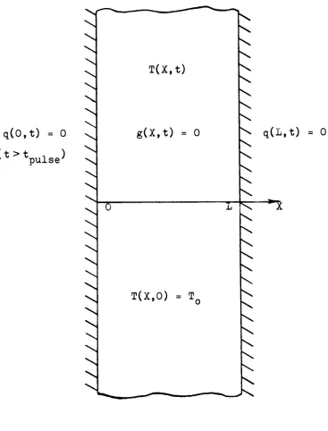
small.

Furthermore,

the

problem considered

herein

is

that

of one

dimensional

heat

conduction

in

a

finite

slab composed of a material with constant

thermal

properties.

The

slab

is

initially

at a uniform

temperature

throughout

and no

internal

heat

generation

is

present.

One

boundary

of

the

slab

is

considered

to

be

insulated for

all

time

and

the

other

boundary

is

subjected

to

a pulse of

heat

flux for

a short period of

time

and

is

then

insulated for

all

time

thereafter.

While

these

boundary

conditions

may

seem

unrealistic,

they

have

been

shown

to

yieldmeaningful results

by

Ozisik

and

Vick

[5]. The

solutions

for insulated

andconvective

boundary

conditions

differ only

in

magnitude and

duration

i.e.,

the

general

trends

of

the

solutions are

identical

for both. These

conditions are

illustrated in

Figure

1.

For these

conditions,

equations

(2.27)

and

(2.28)

q(0,t) =

0

(

t

>

t

,

)

v pulse'

q(L,t) =

0

[image:23.526.70.437.110.592.2]

and

aT ar

ap

p

ar

k

-+ pC + +

-=o

ax2 v

at dx

T

dx

dp

a ar

=

inO<x<Lfort>0

dt T dx

the

initial

and

boundary

_{conditions are}

t =

0,T(x,0)

=

Tn

(3.1)

(3.2)

0 < x < L

and x =

0,

q(0,t) =

Q

sin(a)t) 0 < t.<

-respectively.

q(0,t)=0

x =

L,q(L,t)

= 0

t >

t> 0

3.2

DIMENSIONAL ANALYSIS

In

order

to

simplify

the

subsequent analysis

the

following

dimensionless

quantities are

introduced

u =

T/Tq,

;

dimensionless

temperature

X

= _x/L

;

dimensionless

position x = kx/L2

;

dimensionless

time

b

=

pL/kTo

;

dimensionless

elastic

heat flux

Q

=

qL/kTo ;

dimensionless (total) heat

flux

andk =

k/pCv,

is

the thermal

diffusivity

of

the

material.

Upon

substitution of

these

quantities,

the

governing

equations

become

du du db

b

du

+ + + =0

(3.3)

dX2 dt dX u dX

*

= _Q

-

(3-4)

dl U dX

where a =

AL2/KkTo.

Similarly

the

equation

for

the total

heat

flux

becomes

Q= - +b

ax 311

(3.5)

4.0

FINITE ELEMENT

IMPLEMENTATION

4.1

FUNCTION

APPROXIMATION

The

non-dimensional

form

of

the governing

equations,

as

developed in the

previous

section,

are

a2u au ab b du

(3

3)

- _{+ + + =o}

v '

ax2 _{di ax}

u dX

and

*

= -a

-

(3.4)

dt u dX

The

solution

to the

above

nonlinear, coupled,

partial

differential

equations

is

accomplished via

the

Galerkin

finite

element method

[17].

For this

analysis

linear

elementswere used

for

simplicity.

The

dependent

variables u and

b

are

approximated

by

u(X,t)=

j[

_ip.(X)U.(t)

(4ll)

i i

i=l

and

b(X,t)

=

>

_(p.(X)B.(t)

(4>2)

i i

i=_l

wherevj/i(X) and

$i(X)

are

the

shape

functions,

U;

and

Bi

are

the

nodalvaluesof

the dimensionless

temperature

and

heat flux

respectively

and n

is

the

total

numberof nodes contained

in

the

model.

Figure

2

illustrates

the

form

of

typical

shape

functions

used

for

one-dimensional

linear

elements.

Substituting

(4.1)

and

(4.2)

into

(3.3)

and

(3.4),

respectively

yields

the

X

CM

I

CQ

0)

a

OJ

rH

w

OJ

u

o

<H

OA PI O

H

O

P-4

<D

ft

nJ

J=!

oo

K>

CM

T

j=:

CM

OJ

derivatives

withrespect

to

position and

time,

respectively)

n n n

-y

ipM(X)u.u) +

y

ip.(X)u.(t)+

y

^'.(xjb.w

J- 1 1 J- T1 1 M 1

i=l i=l i=l

n n

+

v1

y

y

ip'.(x)u.(t)<p.(X)B.(t) *o

* < _{i .}

j j i=ij=i

(4.3)

and

v-'

i

^

(4

4)

>

<J>.(X)B.(i)+ qV

>

ip.(X)U.(x) *0 l*'*;

i=l i=l

Note

that

expressions

(4.3)

and

(4.4)

are no

longer

exactly

equal

to

zero since

approximate representation

for

u and

b

are used.

Hence,

(4.3)

and

(4.4)

are

called residuals of

their

original equations.

The

variable Vi present

in both

equations

is

a

function

which

takes

into

account

the non-linearity

i.e.,

1/u

and

is

dependent

upon

the

finite

element node

in

question.

It is

discussed further in

Appendix

A.

4.2

WEIGHTED RESIDUAL

The

next

step in the

finite

element

formulation

ofa problem

by

function

approximation,

is

to

weight

the

residual so

that

it

may

be

set equal

to

zero

again.

This

accomplished

by

selecting

a

weighting

function,

Wk

and

multiplying

each

term

in the

residual

by

it.

The

weighted residual

is

then

integrated

over

the

domain

of

the

continuum

in

question and setequal

to

zero.

The

selection of

the weighting

function determines

the

particular

subcategory

of

the

finite

element method used.

When the weighting

function is

chosen as

ijfK(X),

the

procedure

is

known

as

the

Galerkin

method.

The Galerkin

method

is

highly

popular since

the

selection of

the weighting

function is greatly

general,

each equation

is

multiplied

by

a

different

shape

function.

Different

functions

will

be

shown

in this

analysis,

but

both

are of

the

form

shown

in

Figure

2.

Upon

weighting

and

integrating

over

the

domain,

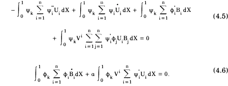
expressions

(4.3)

and

(4.4) become

1 n

VL

1 n

y

v:u.dx +

j

Vk

i

v.u.ax +

1

Vk

i

<p;bi

i=l i=l i=l

dX

(4.5)

f1 + n n ip.V1

V

Y

ip".(p.U.B.dX = ₀

k i _j i _j

i=lj=l

and

1 n

rx n

4>,

y

<J>B.dX + a _<t>,

V'

y

ip'.U.dX = _0.

_ Tk ^ M l Tk J M i

i=_l

(4.6)

i=l

The

order of

the

derivative

in

the

first

term

of equation

(4.5)

can

be

reduced

by

trading

one of

the

differentiations

between the weighting

function,

ipk,

and

the

shape

function,

jjjj.

This is

accomplished

by integrating

the

first

term

by

parts.

Equation

(4.5)

then

becomes

ip'k

y

v'.U.dX-

ipk

I

ipll +

Vk

I

V^dX

i- 1 ' i=l

'_O '_O :_ | r1 n

0 _i=i

1

0 _,=_| +

i=_l

1

0

1 n

i=_l

(4.7)

uj,

V

(b'.B.

dX

+ _ip,

V1

y

y

ip'.cJj.U.B dX = 0.

Tk . _M l

I

a k L MM l J

By

reversing the

order of

the

integration

and summation signs

(4.7)

and

(4.6)

[image:29.526.101.476.192.334.2]

y

i=_l

ipkip.dX

u.+

y

i=_l

ipkip.dX

yi

i=_l

ipk<J>.dX B

(4.8)

and

yi

i=ij=i f1

V ip,ip.cb.dX k i _J

BU

j i

ip.

y

ip.u.

i=_l

y

i=_l

ipk4>.dX

B.

+ a

y

i=l

Vip^dX

k^i U.

= 0.

I

(4.9)

A

morecompact

form for

(4.8)

and

(4.9)

is

and

K,

U. +

C. U.

+

L.,

B. +

W...

BU. =

Q,

ik i ik l lk l ijk _j l ^k

D.,B.

+ aE..U. =0

ik i ik i

(4.10)

(4.11)

where

ik ipkiptdX

(4.12a)

D., ipkip.dX

(4.12b)

ik

VVk<dX

(4.12c)

K. ik

ipkip.'dX

(4.12d)

L ik

ipk<P.dX

(4.12e)

and

n

i=_l

By

multiplying

Wjjk

by

Bj

in

(4.10)

the

equation can

be

expressedas

%

(4.12g)

where

K..U.

+

C.

U. +

L.,

B. + N

U.

=

Q,

ik 1 ik i ik i ik i k

N.. =W.,B..

ik ljk _j

(4.13)

This form

facilitates

the

implementation

of

(4.11)

and

(4.13)

into

a computer

algorithm.

The

details

of

the

integration

necessary

to

form

the

coefficient

matrices

(4.12)

are

found in

Appendix

A.

4.3

TEMPORAL APPROXIMATION

With

(4.11)

and

(4.13)

the

original

governing

equations,

which contained

partial

derivatives

with respect

to

space and

time,

have

been

reduced

to two

sets of

ordinary differential in time.

With

a

further

approximation, the

temporal

derivative

can

be

eliminated

to

obtain

two

sets ofalgebraic equations.

For

first

order

time

derivatives,

the theta

method

is

often employed

[17]. This

methoduses a

finite

difference

scheme

to

represent

the time

derivative

variable

and a

weighting

technique to

obtain an average of

the

dependent

variable at

two

consecutive

time

steps.

For

a single

ordinary

differential

equation of

the

form

x =

flx.t)

the

theta

method

takes

on

the

form

xJ+1_xJ

=

At[9fj+1

where,

At

is

the time

marching

increment,

6,

the weighting

parameter and

the

superscripts

j

and

j

-I-1

indicate

the

valuesof

the

variables ata

time,

t

anda

time

t

-I-At

later,

respectively.

Applying

the theta

method

to

(4.13)

and

(4.11),

the

expressions

become

C

ik

Uj+1-Uj

I I + AtM. ik 8UJ.+1 +

(1-8)UJ

+

AtL

ik

8BJ+ 1

+ (1-8)BJ

= _{At 8} Of1 +

(1-0x4

and D ik

i+1

i i

Bj+1-Bj

+ aAtE ik

euj+1

+

(i-9)u.

i i

where

Mjk

=

Kik

+

Nik.

Solving

(4.14)

and

(4.15)

for

Ulj

+1_and

By

+1

respectively,

yields

(4.14)

(4.15)

C,

+

At9M.,

ik ik

UJ+1

C.

_-At(l-9)M.,

ik ik

UJ

AtGL.,

BJ+i

-At(l-8)L.,

B. + At

ik i ik i

9QJk+1

+

(1-8)04

and

D,BJ+1

= D.,BJ + 1

-aAt(l -6)E,UJ

ik i ik i ik i ik i

(4.16)

(4.17)

Since

the

preceding

systemsofalgebraic equations are

coupled,

they

must

be

solved simultaneously.

Solution is

obtained

by

assuming

a value of one of

the

dependent

variables and

successively

iterating

between

equations until

they

are satisfied within some error

tolerance.

A FORTRAN

program which

performs all of

the

numerical manipulations

necessary

to

construct and solve

the

sets of equations given

by

(4.16)

and

(4.17)

is

found in Appendix B.

When

employing

the

theta

method

for

solution of

first

order

differential

equations,

the

analyst mustchoose a value

for

the

weighting

parameter, theta.

With

theta

equal

to

zero and one

the

familiar forward

the

backward

difference

schemes are recovered.

Comparisons

of solutions

to differential

equations

using

various values of

theta

are performed

in

Reddy

[17]

and

Burden

and

Faires [18]. Both

references

indicate

that

a value of

6

=

\

generally

produces

the

most accurate solution.

When

theta

equals one-half

the

"6"-method

is

generally

known

as

the

Crank-Nicolson

finite

difference

scheme.

In

addition

to

greater

accuracy,

The

Crank-Nicolson

scheme

has

the

additional

benefit

of

being

unconditionally

stable.

For these

reasons

the

Crank-Nicolson

scheme

is

5.0

RESULTS

The

problem of one-dimensional

heat

conduction

in

a

finite

slab was

solved

using the

finite

element method.

From the dimensional

analysis

performed

in

Section

3.0,

all of

the

material properties

have been lumped into

the

dimensionless

parameter

alpha,

a.

Solutions

were obtained

for

different

values ofalpha

to

demonstrate

its

effect on

heat

transfer.

Note

that

for

alpha

equal

to

zero

the

problemreduces

to

that

of classical

heat

conduction.

5.1

TEMPERATURE

RESPONSE

Figure

3

depicts

the temperature

response with respect

to time

at a point

in

the

slab

located

at

X

=

1.0.

The

_response

is

_given

for

_alpha

spanning three

ordersof magnitude

for illustrative

purposes.

For the

lowest

value of

alpha, the

temperature

response exhibits a

behavior

that

is

similar

to

that

predicted

by

the

classical

theory

of

heat

conduction.

However,

the

presence of

the

overshoot

in

the

solution

indicates

that

elastic

heat flux is

present.

Utilizing

the

terminology

associated with

vibratory

mechanical

systems,

it

can

be

said

that

heat

conduction with small values of alpha

is

highly

damped

and

has

a

low

natural

frequency.

For the

intermediate

value ofalpha shown

i.e.,

=

100,

the

oscillatory

behavior

of

the temperature

becomes

more pronounced.

This

trend

continuesasalpha

is

increased.

Increasing

alpha

in

the

governing differential

equations

has

the

effectof

increasing

the

thermal

"stiffness" of

the

slab.

This is

analogous

to

adding

a

stiffer

spring in

a mechanical system.

The

additional stiffness causes

the

natural

frequency

of

the

thermal

response

to

increase

and

it

reduces

the total

~

0=9:6

Z

R:00

LU

OlOlO

O

-:-.-H

:

II

J

II

a!

e>:

e

:

: 1 j3Pj,

H <s

O

CD <IJ

r-t

>

CO

o

H

f.n

3

o

<H

QJ CO

o Pj CO <D

E

OJ

j3

QJ

no

H

shift

in

the

temperature

response

from

a

dissipative

or viscous nature

to

a

conservativeorelastic nature as alpha

increases.

5.2

THERMAL

FLUX

To

further illustrate

the

shift

from

viscous

to

elastic

behavior in

the

thermal response,

Figures

4-6

give

the

heat flux

profiles within

the

slab

for

the

three

valuesofalpha considered above.

Note

that for

each value of

alpha, the

heat fluxes

are shown at

different

instances

of

time.

This

was

done

because

the

thermal

disturbances

travel

at

higher

speeds as alpha

increases.

As defined

in

Section

2.0,

the

total

heat flux is

given

by

the

classical

Fourier

or viscous

term

and

the

newly

introduced

elastic

heat flux.

For

small

alpha,

as

depicted

in

Figure

4,

both

the

viscous and elastic

heat

flux

contribute

significantly

to the

total

flux.

In the

median ranges of

alpha,

the

total

heat flow is

comprised

primarily

of

the

elastic

heat flux

as

illustrated in

Figure

5.

Figure

6

displays

the

heat

flux for large

alpha.

In

this

figure,

the

curves

for

the

total

andelastic

heat

flux

are

nearly identical

indicating

that the

elastic

heat

flow is

the

primary

mode of

heat

conduction.

For

all of

the

flux

plots

shown,

the

total

flux

at

the

boundaries

is

zero or

nearly

zero.

This

agreeswith

the

fact

that

insulated

boundaries

were

imposed

upon

the

slab.

Since both

the

viscousand elastic

heat

fluxes

were computed

using

numerical

approximations,

they

do

not always add

to

yield

exactly

zeroat

the

boundaries.

5.3

THERMAL WAVES

To illustrate

the

propagation of

thermal

waves

in

the

slab,

temperature

profilesatvarious

instants

of

time

are given

in Figures 7-9 for

the

same

three

<

LU

o

CO UJ

o

I

o

Z

LEGEND

ELASTIC

0.4-'%

VISCOUS

/

V*-^*^

^^*

^^s

TOTAL

*

X

0.3- * *

X

* * *

/

\

\

\

0.2-o.i- # _%

-A

#*

*?

-A ?* ?

\

**jm

%3

o.o-* -0.1- 0 * # j

a

-

10.0

-0.2- _?

t

-

0.15

4 0 -0.3 * _*?

%*.

* I I

0.0

0.2

0.4

0.6

0.8

NON-DIMENSIONAL

POSITION

1.0

Figure

4:

Heat Flux Profiles

for

Oi

=

10.0

_and

T~

[image:37.526.48.465.91.644.2]

X

3

<

UJ

X

O

co

Z

UJ

Q

i

Z

O

z

0.2

0.4

0.6

0.8

NON-DIMENSIONAL

POSITION

[image:38.526.54.467.97.659.2]

10.0

X

z>

_l u_

!<

UJ

O

CO

UJ

O

i

Z

O

8.0-

6.0-

4.0-2.0

0.0

-2.0

LEGEND

ELASTIC,,,

a

=

1000.0

t

=

0.025

o.o

0.2

0.4

0.6

0.8

NON-DIMENSIONAL

POSITION

1.0

[image:39.526.49.466.98.645.2]

2.0

oc

ID

!<

QC UJ CL.

1.8

1.6

O

co

Z

UJ

1.4

Q

i

1.2

1.0

LEGEND

r

=

0.01

"t'-OJ""

t""

a

=

10.0

o.o

0.2

0.4

0.6

0.8

NON-DIMENSIONAL

POSITION

1.0

[image:40.526.48.468.89.644.2]

1.6

<

UJ

CL

1.7

UJ

1.6

3

1.5

LEGEND

,

t-

0.01

<#

T^0ff

'"

"6.T"

a

-

100.0

O

CO

UJ

a

1.4

1.3

O

1.2-1.1

1.0

"'.,...

0.2

0.4

0.6

0.8

NON-DIMENSIONAL

POSITION

1.0

[image:41.526.50.468.87.647.2]

1.5

1.4-LU CSC oc UJ a. UJ

O

CO i

LEGEND

t

=

0.01

"t"""0.05"'

a

=

1000.0

1.3

1.2- 1.1-- _* '. * '. c 1 i -^ -* i * -i t -' -t n ^ t ^ : c '. -i s ' -*

* " _>

? ''

? ^^^

.

1.0

dm

0.6

0.8

1.0

NON-DIMENSIONAL

POSITION

[image:42.526.47.462.93.642.2]

applied pulse

through

the

slab prior

to

being

reflected

by

the

right surface of

the

slab.

A

previous remark

regarding

the

increase

in

wave propagationspeed

with

increasing

alpha

is

clearly

shown

in this

series of

figures.

For

eachvalue

ofalpha

considered, the thermal

wave reaches

the

right wall

in

a

progressively

shorterperiod of

time.

In

all

three

figures,

the temperature

profile

is

given

for

x =

0.01.

For this

instant

of

time,

the thermal

pulse

is

observed

to

penetrate

deeper into

the

slab

for higher

valuesofalpha.

These

two

facts

verify that

the

thermal

wave propagation speed

increases

as alpha

does.

This

ties

into

the

observation

that the thermal

"stiffness"

increases

with alpha.

The

propagation speed of sound waves

in

a

solid

increases

as

the

stiffness or more

precisely the

elastic

modulus,

of

the

material

increases.

The

results of

this

analysis

indicate

that

the

propagation

speed of

the

thermal

waves

increases

as

the

thermal

"stiffness" of

the

slab

material

increases.

Since

these

results concur with

those

for

first,

or

ordinary,

sound waves

in

a

solid, the

analogy between

thermal

and mechanical wave

propagation

becomes

more apt.

Figures

7-9

also providesome

information

on

the

viscous/elastic nature of

the

heat flow

within

the

slab.

For

low

alpha, the thermal

wave

is

wide and

small

in

amplitude

indicating

that the

applied pulse

has

largely

diffused

out

in

the

slab.

As

the

alpha

increases

the thermal

wave

becomes

more well

defined

i.e.,

it

reduces

in

width and

increases

in

amplitude.

This is

due

to the

presence

of a

larger

elastic

heat

flux

which requires a

longer time

to

decay.

Figure

10

shows

the thermal

wave after

it has

reflected off

the

right

boundary

of

the

slab.

Note

that

the

maximum amplitude of

the

wave

has decreased

and

the

minimum

temperature

in the

slab

has increased. As

the

thermal

wave

travels

UJ

(jC

ID

!<

ac UJ cl

1.5

1.4-

1.3-<

Z

O

CO

LU

1.2

i

1.1-1.0

*

LEGEND

t

=

0.055

V="6.065"

ex

=

1000,0

.,

o.o

0.2

0.4

0.6

0.8

NON-DIMENSIONAL POSITION

1.0

Figure

10:

Temperature

Profiles

f

or

CX

=

1000.0

[image:44.526.55.463.91.627.2]

of

the

material

in

its

wake.

This

phenomenon continues until

the

wave

has

completely

dissipated

and

the

slab reaches a uniform

temperature.

5.4

FINITE

ELEMENT

PROGRAM

Before

making any

final

conclusions,

some comments on

the

finite

element model and

the

FORTRAN

code used

to

solve

the

problem ofthermal

wave propagation are

in

order.

Since

one-dimensional

heat

transfer

is

assumed, the

finite

element model

simply

consists of a

string

of

one-dimensional

"line"

elements.

The

program allows

the

slab

to

be divided

into

any

number of uniform size elements.

The

number ofelements used

in the

analysis was varied

to

observe

its

effecton

the

solution.

For

smallmodelsoften

to

twenty

elements,

convergencewas

very

rapid

i.e.,

within

five

iterations. The

small models also allowed a

large

time

marching

increment

to

be

used while

still

maintaining

a

fast

convergence rate.

Unfortunately,

these

models

do

not

yield enough

information

within

the

slab

to

produce acceptable

figures

without

curve

fitting.

A

mediumsize model of

fifty

elements was used

exclusively

to

produce all

the

figures

within

this

work.

The

convergence rate

for

this

size model

is

also

acceptable

but is

highly

dependent

on

the

time

marching

interval.

For

time

intervals

on

the

order of

0.01

dimensionless

time units,

convergence could not

be

obtained within

the

maximum number of

iterations

allowed.

The

maximum

numberof

iterations

built

into

the

code serves as a

safety

to

prevent an

infinite

loop

situation.

Due

to

the

large

number of mathematical manipulations

required

for

each

iteration,

the

iterations

are

limited

to

amaximum of

100.

A

time interval

of

0.001

dimensionless

time

units produced convergence within

alpha required

the

largest

number of

iterations

and

therefore

were used

to

judge

convergence rates.

Time intervals

on

the

order of

0.0001

units yielded

rapid convergence.

In

order

to

keep

the

total

number of

iterations

to

a

minimum

(total

iterations

is

given

by

the

number of

iterations

at each

time

step

multiplied

by

the

number of

time

steps) a

time marchng

increment

of

0.005

non-dimensional

time

units was utilized.

Convergence

with

this

increment

was

within

five iterations

ateach

time

step.

Large

models of

100

elements were experimented with

briefly.

The

results

from

these

models were not

any

different from

an

accuracy

point-of-view, than

the

medium sized model.

However,

when

using

this

number of

elements,

a much smaller

time marching

increment,

than

those

discussed

above,

had

to

be

used.

This,

coupled with

the

fact

that the

number of

mathematical operations performed at each

iteration

is

a cubic

function

of

the

number of elements

used,

requires

large

amounts of computer

time

to

obtain

the

entire solution.

For this

reason

the

major portion of

the

analysis was

performed

using

a medium sized model.

Mention

was made

in

section

4.0

that the

solution was obtained

by

successively

iterating

between

the

two

systems of equations until a

convergence criteria was satisfied.

The

criteria used

for

convergence was

that

the

difference

between

temperatures

obtained at subsequent

iterations

be less

than

a specified

tolerance.

Since

the

temperature

varies at each

node,

and

infinite

norm of

the temperature

difference

at respective nodes

is

obtained

to

determine

the

maximumchange

in

temperature

betwen

iterations.

When this

value of

the

infinite

norm of

the temperature

"vector"

becomes less

than the

convergence

tolerance

used

in

the

FORTRAN

code was

5X(10)-6.

Note

that

is

the

smallestvalue

that

can

be

usedwithsingleprecision computer arithmetic.

The final

portionof

the

discussion deals

with

the

applied

temperature

flux

at

the

left boundary.

Two

general

types

of

functions

were experimented

with,

namely

a

step

input

anda

half-sine

pulse

input. The

amplitudeand

duration

of

the

pulse

input

were varied

to

observe

their

effect on

the thermal

response.

The

results were again analogous

to those

of a mechanical system

i.e.,

the

amplitude and

frequency

of

the thermal

oscillations varied as

the

input

pulse

was modified.

For

all of

the

figures

presented

in

this

section a pulse with an

amplitude of

10.0

dimensionless

heat flux

units was used.

The step input

was

used

to

verify that the

computer code was

functioning

properly

and

hence

no

6.0

CONCLUSIONS

From

the

foregoing

analysis,

it has been

shown

that

it is

possible

to

modify the

classical

diffusion

equation

to

account

for

thermal

wave

propagation.

This is

accomplished

by including

a second

term

in

Fourier's law

of

heat

conduction.

This

second

term

has

been

called

the

"elastic"

heat flux

vector

due

to

the oscillatory

behavior

of

the temperature

within

the

media.

The

nature of

the

solution

to

the

proposed

governing

equations

intimate

that

the

methodology

used

herein is

plausible.

However,

no experimental evidence

exists

to

verify

or

dispute

this.

In

order

to

perform such a

comparison, the temperature

field

within an

insulated

slab at consecutive

instances

of

time

is

needed.

For

a quasi-static process

occuring in

a conventional media such as a

metal, this

data is

easily

obtainable.

Aquisition

of

this

same

data

in

a material

that

promotes

thermal

wave propagation

is

precluded

for

the

following

reason.

Thermal

waves

have

been

observed

only in

materials with

highly

orderedmicrostructures

devoid

of

impurities

or

discontinuities.

The

presence of a

temperature

sensing

probe

within such amaterial would

introduce

a

discontinuity

thereby

disrupting

the

flow

of

any

thermal waves.

Some data

could

be

acquired

by

using temperature

probes at

the

boundaries

of

the

media

to

observe

temperature

fluxuation

with

time

at a single point.

With

this

in

formation,

the

dimensionless

parameter, a,

could

be

changed

by

varying the individual

quantities which constitute

it.

two

setsof

data

should

follow

the

trends

presented

in

the

previous section

if

the

proposed

governing

_{equations are correct.}

Possible

extensions

to the

work

done

in

this thesis

is

the

solution of

the

governing

equations

in

two

dimensions.

Such

a solution could provide

information

on whether

thermal

waves exhibit constructive/destructive

interference

like

other more

familiar

waves.

This

could

further

the analogy

betwen

first (ordinary)

andsecond

(thermal)

waves.

Another

obviousextension

would

be

performing

experiments while

varying

the

parameter alpha as

REFERENCES

[1]

Peshkov,

V.

'"Second

Sound'

in

Helium

II."

Journal

of

Physics

(USSR)

8

(1944):

381.

[2]

Ackerman, CC,

Bertman

B.,

Fairbank

H.A.,

and

Guyer,

R.A. "Second

Sound

in

Solid

Helium."

Physical Review Letters

16

(1966):

789.

[3]

Bertman,

B.

and

Sandiford,

D.J. '"Second

Sound'

in Solid

Helium."

Scientific American

May

1970,

pp.

92-101.

[4]

Lord,

N.W.

and

Shulman,

Y.

"A

Generalized

Dynamical

Theory

of Thermoelasticity."

Journal

of

Mechanical Physics

in

Solids

15

(1967): 299.

[5]

Ozisik,

M.N.

and

Vick,

B. "Propagation

and

Reflection

of

Thermal

Waves

in

a

Finite

Medium."

Journal

of

Heat

and

Mass Transfer

27

(1984): 1845-54.

[6]

Bogy,

D.B.

and

Naghdi,

P.M.

"On

Heat Conduction

and

Wave

Propagation in Rigid

Solids."

Journal

of

Mathematical Physics

11

(1970): 917.

[7]

Gurtin,

M.E.

and

Pipkin, A.C,

"A

General

Theory

of

Heat Conduction

with

Finite Wave

Speeds."

Archives

for

Rational Mechanics

and

Analysis 31 (1968): 113.

[8]

Green,

A.E.

and

Naghdi,

P.M. "The Second

Law

of

Thermodynamics

and

Cyclic

Processes."

Journal

of

Applied Mechanics

45

(1978): 487.

[9]

Atkin, R.J., Fox,

N.

and

Vasey,

M.W.

"A

Continuum

Approach

to

the

Second

Sound

Effect."

Journal

of

Elasticity

5 (1975):

237-48.

[10]

Coleman,

B.D.

and

Noll,

W. 'The

Thermodynamics

of

Elastic

Materials

with

Heat

Conduction

andViscosity."

Archives

for

Rational

Mechanics

and

Analysis

13

(1963): 167.

[11]

Kratochvil,

J.

and

Dillon,

O.W. "Thermodynamics

of

Elastic-Plastic

Materials

as a

Theory

with

Internal

State

Variables."

Journal

of

Applied Physics 40

(1969): 3207.

[12]

Mase,

G.E.

Continuuum

Mechanics,

Shaum's Outline Series

in

Engineering,

New York:

McGraw-Hill Book

Company,

1970,

p.

131.

[13]

Karlekar,

B.V.

Thermodynamics

for Engineers. Englewood

Cliffs:

Prentice-Hall,

Inc.,

1983,

p.

422.

[15]

Chester,

M.

"Second Sound

in

Solids."

Physics Review 131 (1963):

2013-15.

[16]

Green,

A.E.

and

Naghdi,

P.M.

"A

General

Theory

of an

Elastic-Plastic

Continuum."

Archives for Rational

Mechanics

and

Analysis 18

(1965): 251-81.

[17]

Reddy,

J.N. An Introduction

to

the

Finite Element Method. New York:

McGraw-Hill Book

Company,

1984.

[18]

Burden,

R.L.

and

Faires,

J.D.

Numerical Analysis. 3rd

ed.

Boston:

APPENDIX

A

In

this section, the

details

of

the

formation

of

the

systemmatrices will

be

expanded upon.

The final form

of

the

weighted residuals given

in Section

4.0

were <