International Journal of Innovative Technology and Exploring Engineering (IJITEE) ISSN: 2278-3075, Volume-8 Issue-6S, April 2019
Abstract— Testing plays a vital role in Software industries. Of all the methods, Combinational Testing is most preferred due to its robust approach in testing each and every possible pair, triple or n-way of a configuration at least once. Most of the faults occurred through these interactions between components can be captured using pairwise Testing. Many of the existing research proposes novel methods which aims to find a test set of configurations to cover all the possible different pairs. The difficulty of solving this problem is demonstrated to be NP-Complete.
In this paper we propose to deeply explore the usage of Simulated Annealing, a meta heuristic algorithm to pairwise testing that generates the least number of test configurations with the aim to cover all distinct pairs possible. Furthermore, we proposed a fitness function which is dynamic in nature. This provides us the flexibility of choice between the runtime of this algorithm and the different pairs coverage of the test configurations generated. An ideal scenario would be a combination of both (runtime and coverage), but the results show that they are inversely related.
Keywords— Meta-heuristic algorithms, Simulated annealing, Combinatorial Testing, Pairwise Testing
I. INTRODUCTION
In component-based development, a big application is created by integrating smaller components which have already been developed earlier, possibly for a different project in the past [7]. This greatly reduces the time and cost required to create a new application. At every step of integration process, a great number of components interact with each other in desired manner thereby producing the expected results. Often this scenario of interaction between components is error prone and the testing techniques chosen by developers plays a vital role in making the interaction error free. Hence, to deliver a quality software, effective and efficient testing is the key. For complex systems, testers have the constraints of time and money, hence the idea of testing each and every possible configuration cannot be feasible [1]. Therefore, effective testers should choose a part or a subset of the test configurations for testing such that the system is vastly tested, but with a minimal number of configurations thereby saving time and money [6]. Researchers relate this scenario with that of minimum set coverage problem to show that it is indeed NP-complete [15].
Pairwise Testing is one of the most popular methods used in today’s software industries to test the robustness of a program thoroughly [10, 12]. It is the most commonly used form of combinatorial testing. The idea is to capture all
Revised Manuscript Received on April 03, 2019.
M.V.Prudhvi Raj, BITS-Pilani, Hyderabad Campus Hyderabad, Telengana-500078
Subhrakanta Panda, BITS-Pilani, Hyderabad Campus Hyderabad, Telengana-500078
possible discrete pairs of an input given to a software application at least once. The reason being
Table 1:Parameters involved in the Application
Scripting Language Web Server Browser
Java Script Apache Chrome
vbScript IIS Firefox
Perl PWS Opera
majority of the errors are caused by a single input parameter or a combination of two [3, 5, 12].
For example, let’s consider a portal system consisting of three components namely scripting language, web servers and browsers as demonstrated in Table 1. consider the portal to be developed in three scripting languages JavaScript, VbScript and Perl. Uses either of three web server Apache, IIS or PWS and may view the portal using browsers such as Chrome, Firefox and Opera. For a System tester, a test configuration comprises of these three components such as {JavaScript, Apache, Chrome} or {VbScript, IIS, Firefox} [6]. The total number of possible configurations in this scenario are 3*3*3 = 27. For an application of this size having 27 different configurations, it’s possible to test all the discrete combinations of configurations, but supposing an application consists of 10 components each having 4 different possibilities. Then total number of distinct possible configurations are 410 = 1,048,576. This would be a very tedious and almost an impossible task for the testers to choose a subset of 1,048,576 configuration such that all the different pairs can be covered. Existing methods to solve this problem can be broadly classified into algebraic construction, Greedy approach and meta-heuristic search.
Objective
Based on the above motivation discussed in the form of an example in Section 1, we fix the objective of this paper as to minimize the number of test configurations required to cover all the possible different pairs of the given input parameters using pairwise testing. Considering all the configurations of existing parameters would be exponential in number for any given application. Hence, we use a meta-heuristic search algorithm to select only those configurations which yield maximum number of different pairs. To achieve this, we use a meta-heuristic algorithm "Simulated Annealing"[8] with certain modifications to the Fitness function, thus gaining control over the algorithms run time as well as the coverage of different pairs possible.
Simulated Annealing: An Experimental
Application on Pairwise Testing
The rest of this paper is as follows. In Section 2, we discuss the simulated annealing meta heuristic technique, along with its applicability to pairwise testing, its fitness function and the acceptance or rejection criteria. In Section 3, we discuss the results of our proposed algorithm for pairwise testing.
II. META-HEURISTIC ALGORTHMS Often in computer science and mathematical optimization, finding the global optimum of a particular set or a function is a difficult and computationally hard problem to solve for. The standard search-based algorithms (linear search algorithms) searches the whole sample space provided in order to find the global optimum and gives its precise value, but when the sample space is too large, it is computationally expensive and has a huge effect on the time complexity. Hence to overcome these difficulties, Meta-heuristic algorithms are often preferred. The goal is to minimize the time complexity and find a better approximation to global optimum. In this paper, we choose simulated annealing algorithm to search the sample space of configurations provided by Pairwise testing technique on any given application.
A. Simulated Annealing
Simulated annealing [13] is a probabilistic technique for approximating the global optimum of a given function [14, 16]. It is a meta heuristic which approximate the global maximum/minimum in a large search space provided. To be precise the search space provided to this meta heuristic is discrete in nature.
This technique was initially used in metallurgy involving heating and controlled cooling of a materials to increase the size of its crystals and reduce the defects [4]. The basic idea is to accept worse solutions in order to search for the global optimum instead of getting struck with the local optimum. The algorithm for simulated annealing works as follows [11].
1. Set temperature T a high value and cooling factor CF to a decimal value between (0,1).
2. Randomly generate a solution Si from the given sample space.
3. Calculate the cost of the generated solution using some cost function defined.
4. Generate another solution Sj randomly and calculate its cost.
5. If CSj > CSi accept the new solution with a certain probability P.
6. If CSj <= CSi accept the new solution.
7. Reduce the temperature by multiplying it with the cooling factor.
8. Repeat the steps from 2-7 until the desired solution is found or until temperatures reaches to zero.
B. Simulated Annealing for Pairwise Testing
To demonstrate how simulated annealing is applied to pairwise testing, let us consider an application for example that has four different parameters, each with different number of variables to be tested as:
P1: Browser: - Internet Explorer, Firefox, Opera mini and Safari
P2: Screen Resolution: - 800*600, 1024*768 and 1200*800
P3: JavaScript: - JSEnabled and JSDisabled
P4: Cookies: - CKEnabled and CKDisabed
Let us number these parameter variables starting from 0 as P1: <0-3>, P2: <4-6>, P3: <7-8>, P4:<9-10>. To demonstrate these labeling, we consider a possible test configuration (Internet Explorer, 1024*768, JSEnabled, CKDisabled). This can be represented as (0,5,7,10). This representation helps us in identifying the unique pairs covered by the test configuration generated. We carry on this example to demonstrate the working of fitness function and the acceptance or rejection criteria for our proposed method.
C. Fitness Function
The purpose of using Simulated annealing is to reduce the number of test configurations required to test the given soft-ware system exhaustively by pairwise testing. To successfully achieve this, we have to select a certain number of configurations from the set of all possible distinct configurations available. Fitness Function thus helps us to decide on weather a randomly chosen test configurations should be picked or not.
The fitness function we consider here is the total number of different pairs a randomly picked test configuration can generate. This is a straight forward assessment as to how many pairs are covered by a randomly generated test configuration and weather to accept it or reject it. Consider a test configuration (0,5,7,10) from the above example in Section 2B. The possible pairs that can be generated are 4C2 = 6. They are {(0,5), (0,7), (0,10), (5,7), (5,10), (7,10)}. To generalize the fitness function for a n-parameter test case, the possible pairs would be nC2.
Consider a case where we have two test configurations from the example mentioned in Section 2.1. Let the configurations be (2,5,7,9) and (2,5,8,10). The number of pairs covered by the first test configuration are 6 while the number of pairs covered by the second test configuration are 5. This is due to the fact that the pair (2,5) has already been covered by the first test configuration. We only consider the total number of different pairs covered by a randomly choose test configuration to judge whether it gets accepted or rejected.
D. Acceptance or Rejection Criteria
Given any randomly chosen test configuration of an application involving N-parameters, the following rules helps us decide whether to accept or reject the configuration. Also, the total number of different pairs covered by an ideal test are nC2.
1. If the total number of different pairs covered by a test configuration are equal to the maximum number of different pairs that can be covered by an ideal test configuration, accept it.
International Journal of Innovative Technology and Exploring Engineering (IJITEE) ISSN: 2278-3075, Volume-8 Issue-6S, April 2019
3. If the total number of different pairs covered by a test configuration are less than half of the different pairs covered by an ideal test configuration, reject it. To calculate the probability by which we accept/reject a test configuration, we follow the below rules.
1. Let MP be the maximum distinct pairs that an ideal test configuration can generate.
2. let DP be the number of distinct pairs covered by a randomly generated test configuration and DP greater than equal to nC2.
3. Let δ = MP - DP. The probability P is calculated as P = exp(-δ/T).
4. Generate P`, a random value between (0,1). 5. If P` < P, accept the test configuration else reject it. The Probability of acceptance is greater at higher temperatures and gradually reduces as the temperature decreases. Those test configurations which cover the maximum number of different pairs possible are accepted at higher temperatures, but as the temperature decreases, the test configurations which gets rejected couldn’t cover n
C2/2 different pairs and we end up waiting in the loop. This Scenario does not occur often, but then due to the randomness of the algorithm proposed, it is an equally likely outcome of all the possible outcomes. Hence, we multiply the cooling factor to our acceptance criteria, i.e. Accept a test configuration if the number of distinct pairs covered are greater than or equal to coolingfactor*(nC2/2).
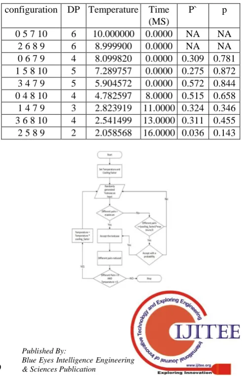
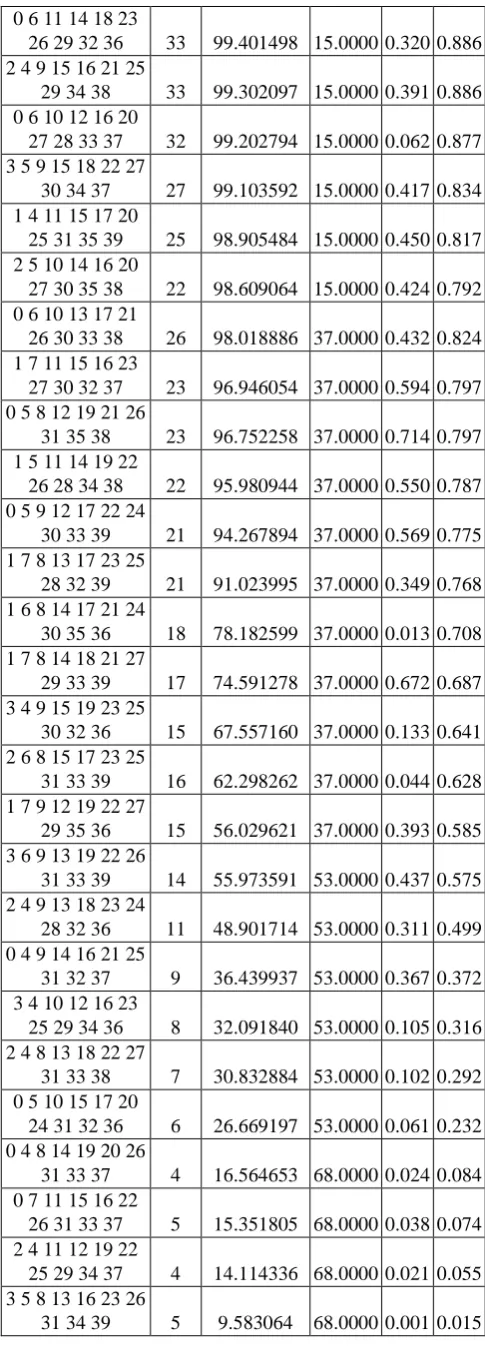
The above modification to the fitness function also serves as a controlling mechanism on the end result. By tightening our fitness function, i.e., choosing a cooling factor as close to 1 as possible will make the algorithm run a much longer time but the number of configurations selected to cover all the possible different pairs would be minimum in number. On the contrary, if we choose cooling factor that tends to approach 0, the algorithm will run much faster but results in a greater number of test configurations to cover all the distinct pairs possible. Finally, the stopping criteria of the algorithm would be when all the possible different pairs are covered by the test configurations generated or when the temperature reaches zero. Refer to the flowchart of the proposed algorithm in Figure 1 for better understanding.
III. RESULTS
The proposed algorithm has been tested exhaustively by considering different sizes of applications and varying the number of parameters involved. For understanding purposes, Let’s see the results of the proposed algorithm when applied on the example discussed in Section 2.1. The total number of different pairs possible are 4×3+4×2+4×2+3×2+3×2+2×2 = 44. The configurations selected by the proposed algorithm are listed in Table 2. When we tighten the fitness function by choosing the value of cooling factor as 0.99999 it gives 100% coverage i.e., we have covered all the 44 different pairs with those 12 configurations generated but notice that the time taken by is approximately 38 Milli seconds. We see the resultant output from Table 3 and Table 4 when the cooling factor is decreased to 0.89999 and 0.79999 respectively.
Therefore, to achieve a 100% coverage with minimum test configurations, we take a toll on the run time of the
algorithm. On the contrary, if runtime of the proposed algorithm is prioritized, we end up having a certain number of configurations which are minimum in number with respect to the percentage of coverage achieved. Therefore, coverage and runtime are inversely proportional as observed by the results.
[image:3.595.305.548.245.425.2]For a better understanding, let us see the results of the proposed algorithm when applied to an example discussed in Section 1. We considered an application with 10 different components and each component having 4 different possibilities to discuss the scale of difficulty in terms of time and complexity. As mentioned in Section 1 the total number of distinct possible configurations are 410 = 1,048,576, the
Table 2: 12 configurations with 100% coverage at T = 10, CF = 0.99999 and runtime = 38ms
configuration DP Temperature Time (MS)
P` p
0 4 7 9 6 10.000000 0.0000 NA NA
2 6 7 9 5 9.999900 0.0000 0.627 0.905
1 4 8 10 6 9.999800 0.0000 NA NA
1 6 8 10 3 9.999600 0.0000 0.571 0.741
2 5 8 9 5 9.999400 0.0000 0.715 0.905
3 6 7 10 4 9.999300 0.0000 0.127 0.819
3 5 8 10 3 9.998700 0.0000 0.070 0.741
1 5 7 9 4 9.993002 0.0000 0.239 0.819
0 6 8 10 3 9.990604 0.0000 0.411 0.741
2 4 8 10 2 6.666287 16.0000 0.098 0.549 3 4 7 9 2 6.663954 22.0000 0.437 0.549 0 5 8 9 1 3.332356 22.0000 0.061 0.223
Table 3: 9 configurations with 88.7% coverage at T = 10, CF = 0.89999
configuration DP Temperature Time (MS)
P` p
0 5 7 10 6 10.000000 0.0000 NA NA
2 6 8 9 6 8.999900 0.0000 NA NA
0 6 7 9 4 8.099820 0.0000 0.309 0.781
1 5 8 10 5 7.289757 0.0000 0.275 0.872
3 4 7 9 5 5.904572 0.0000 0.572 0.844
0 4 8 10 4 4.782597 8.0000 0.515 0.658
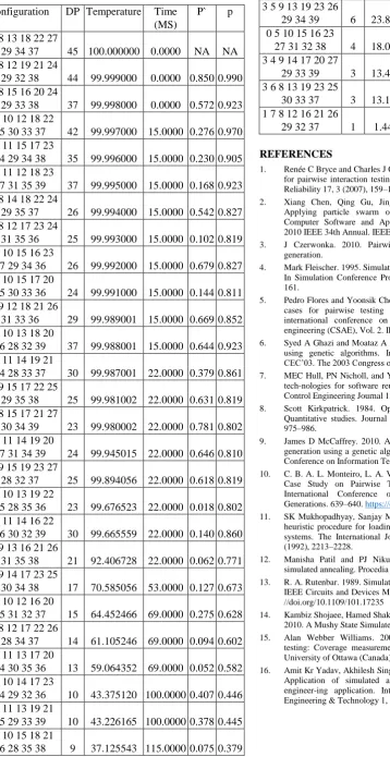
[image:3.595.304.550.452.834.2]total number of distinct possible pairs are 720. From Table 5, we have achieved a 98.33% coverage at cooling factor (CF) set at 0.999 i.e., the proposed algorithm covered 708 distinct pairs just by choosing 33 of the 410 distinct configurations possible with a runtime of 60ms. The same example when ran at a cooling factor (CF) set at 0.99999 achieved a 99.86% coverage i.e., it covered 719 of the 720 distinct pairs possible in a run time of 300ms from Table 6.
Manisha Patil and P.J. Nikumb also have proposed the use of simulated annealing for pair wise testing, but the results shown[12] were only limited to finding a test set best suitable for a given problem only and the size of the test set was not specified. Hence, a comparison of results could not be made.
IV. FUTURE WORK
Combinatorial testing can greatly reduce the cost of the software testing while still keeping high fault detection ability. However, building optimal combinatorial test suites is an NP-complete problem and remains an open area for research. In this paper, we applied Simulated Annealing to provide minimal number of configurations which would cover all the possible different pairs. Our experimental results show the effectiveness and the efficiency of our approach.
In future, we plan to implement the proposed algorithm using parallel computing to reduce the runtime much further and also apply the proposed algorithm on real world application testing to detect faults.
Table 4: 11 configurations with 91% coverage at T = 100, CF = 0.79999
configuration DP Temperature Time (MS)
P` p
0 4 7 9 6 100.000000 0.0000 NA NA
0 5 8 9 5 79.999000 0.0000 0.356 0.988 2 6 7 9 5 63.998400 0.0000 0.411 0.984 2 5 7 10 5 51.198080 16.0000 0.062 0.981 1 5 7 9 3 40.957952 16.0000 0.014 0.929
3 4 8 10 6 32.765952 16.0000 NA NA
1 4 8 9 2 26.212434 16.0000 0.384 0.858 2 4 8 9 2 20.969685 16.0000 0.290 0.826 3 6 8 10 3 10.736076 16.0000 0.219 0.756
Table 5: 33 configurations with 98.33% coverage at T =100, CF = 0.999 and runtime of 69 ms configuration DP Temperature Time
(MS)
P` p
3 7 10 13 19 23
24 28 32 38 45 100.000000 15.0000 NA NA 2 4 10 12 18 22
26 31 34 37 45 99.900000 15.0000 NA NA
3 7 11 15 18 21
25 28 35 36 42 99.800100 15.0000 0.158 0.970 0 5 10 13 16 20
26 31 35 36 40 99.700300 15.0000 0.014 0.951 3 5 9 14 17 20 25
29 34 39 43 99.600600 15.0000 0.054 0.980 0 7 11 13 17 20
24 29 34 37 31 99.500999 15.0000 0.387 0.869
0 6 11 14 18 23
26 29 32 36 33 99.401498 15.0000 0.320 0.886 2 4 9 15 16 21 25
29 34 38 33 99.302097 15.0000 0.391 0.886 0 6 10 12 16 20
27 28 33 37 32 99.202794 15.0000 0.062 0.877 3 5 9 15 18 22 27
30 34 37 27 99.103592 15.0000 0.417 0.834 1 4 11 15 17 20
25 31 35 39 25 98.905484 15.0000 0.450 0.817 2 5 10 14 16 20
27 30 35 38 22 98.609064 15.0000 0.424 0.792 0 6 10 13 17 21
26 30 33 38 26 98.018886 37.0000 0.432 0.824 1 7 11 15 16 23
27 30 32 37 23 96.946054 37.0000 0.594 0.797 0 5 8 12 19 21 26
31 35 38 23 96.752258 37.0000 0.714 0.797 1 5 11 14 19 22
26 28 34 38 22 95.980944 37.0000 0.550 0.787 0 5 9 12 17 22 24
30 33 39 21 94.267894 37.0000 0.569 0.775 1 7 8 13 17 23 25
28 32 39 21 91.023995 37.0000 0.349 0.768 1 6 8 14 17 21 24
30 35 36 18 78.182599 37.0000 0.013 0.708 1 7 8 14 18 21 27
29 33 39 17 74.591278 37.0000 0.672 0.687 3 4 9 15 19 23 25
30 32 36 15 67.557160 37.0000 0.133 0.641 2 6 8 15 17 23 25
31 33 39 16 62.298262 37.0000 0.044 0.628 1 7 9 12 19 22 27
29 35 36 15 56.029621 37.0000 0.393 0.585 3 6 9 13 19 22 26
31 33 39 14 55.973591 53.0000 0.437 0.575 2 4 9 13 18 23 24
28 32 36 11 48.901714 53.0000 0.311 0.499 0 4 9 14 16 21 25
31 32 37 9 36.439937 53.0000 0.367 0.372 3 4 10 12 16 23
25 29 34 36 8 32.091840 53.0000 0.105 0.316 2 4 8 13 18 22 27
31 33 38 7 30.832884 53.0000 0.102 0.292 0 5 10 15 17 20
24 31 32 36 6 26.669197 53.0000 0.061 0.232 0 4 8 14 19 20 26
31 33 37 4 16.564653 68.0000 0.024 0.084 0 7 11 15 16 22
26 31 33 37 5 15.351805 68.0000 0.038 0.074 2 4 11 12 19 22
25 29 34 37 4 14.114336 68.0000 0.021 0.055 3 5 8 13 16 23 26
[image:4.595.304.547.51.737.2]International Journal of Innovative Technology and Exploring Engineering (IJITEE) ISSN: 2278-3075, Volume-8 Issue-6S, April 2019
Table 6: 33 configurations with 99.86% coverage at T =100, CF = 0.999999 and runtime of 300 ms configuration DP Temperature Time
(MS)
P` p
0 6 8 13 18 22 27
29 34 37 45 100.000000 0.0000 NA NA
3 4 8 12 19 21 24
29 32 38 44 99.999000 0.0000 0.850 0.990 0 5 8 15 16 20 24
29 33 38 37 99.998000 0.0000 0.572 0.923 2 7 10 12 18 22
25 30 33 37 42 99.997000 15.0000 0.276 0.970 1 4 11 15 17 23
24 29 34 38 35 99.996000 15.0000 0.230 0.905 0 4 11 12 18 23
27 31 35 39 37 99.995000 15.0000 0.168 0.923 2 5 8 14 18 22 24
29 35 37 26 99.994000 15.0000 0.542 0.827 3 5 8 12 17 23 24
31 35 36 25 99.993000 15.0000 0.102 0.819 2 4 10 15 16 23
27 29 34 36 26 99.992000 15.0000 0.679 0.827 1 4 10 15 17 20
25 30 33 36 24 99.991000 15.0000 0.144 0.811 1 5 9 12 18 21 26
31 33 36 29 99.989001 15.0000 0.669 0.852 3 7 10 13 18 20
26 28 32 39 37 99.988001 15.0000 0.644 0.923 1 6 11 14 19 21
24 28 33 37 30 99.987001 22.0000 0.379 0.861 0 7 9 15 17 22 25
29 35 38 25 99.981002 22.0000 0.631 0.819 1 7 8 15 17 21 27
30 34 39 23 99.980002 22.0000 0.781 0.802 2 7 11 14 19 20
27 31 34 39 24 99.945015 22.0000 0.646 0.810 3 5 9 15 19 23 27
28 32 37 25 99.894056 22.0000 0.618 0.819 0 6 10 13 19 22
25 28 35 36 23 99.676523 22.0000 0.018 0.802 3 6 11 14 16 22
26 30 32 39 30 99.665559 22.0000 0.140 0.860 2 4 9 13 16 21 26
31 35 38 21 92.406728 22.0000 0.062 0.771 0 6 9 14 17 23 25
30 34 38 17 70.585056 53.0000 0.127 0.673 1 6 10 12 16 20
25 31 32 37 15 64.452466 69.0000 0.275 0.628 1 4 8 12 17 22 26
28 34 37 14 61.105246 69.0000 0.094 0.602 1 5 11 13 17 20
24 30 35 36 13 59.064352 69.0000 0.052 0.582 2 7 10 14 17 23
24 29 32 36 10 43.375120 100.0000 0.407 0.446 3 5 11 13 19 21
25 29 33 39 10 43.226165 100.0000 0.378 0.445 0 6 10 15 18 21
26 28 35 38 9 37.125543 115.0000 0.075 0.379
2 6 9 15 16 22 24
28 32 39 6 26.538952 122.0000 0.092 0.230 3 5 9 13 19 23 26
29 34 39 6 23.855458 138.0000 0.163 0.195 0 5 10 15 16 23
27 31 32 38 4 18.069251 153.0000 0.050 0.103 3 4 9 14 17 20 27
29 33 39 3 13.436705 169.0000 0.027 0.044 3 6 8 13 19 23 25
30 33 37 3 13.139067 169.0000 0.007 0.041 1 7 8 12 16 21 26
29 32 37 1 1.446055 285.0000 0.000 0.000
REFERENCES
1. Renée C Bryce and Charles J Colbourn. 2007. The density algorithm for pairwise interaction testing. Software Testing, Verification and Reliability 17, 3 (2007), 159–182.
2. Xiang Chen, Qing Gu, Jingxian Qi, and Daoxu Chen. 2010. Applying particle swarm optimization to pairwise testing. In Computer Software and Applications Conference (COMPSAC), 2010 IEEE 34th Annual. IEEE, 107–116.
3. J Czerwonka. 2010. Pairwise testing, combinatorial test case generation.
4. Mark Fleischer. 1995. Simulated annealing: past, present, and future. In Simulation Conference Proceedings, 1995. Winter. IEEE, 155– 161.
5. Pedro Flores and Yoonsik Cheon. 2011. PWiseGen: Generating test cases for pairwise testing using genetic algorithms. In IEEE international conference on computer science and automation engineering (CSAE), Vol. 2. IEEE Shanghai, 747–752.
6. Syed A Ghazi and Moataz A Ahmed. 2003. Pair-wise test coverage using genetic algorithms. In Evolutionary Computation, 2003. CEC’03. The 2003 Congress on, Vol. 2. IEEE, 1420–1424. 7. MEC Hull, PN Nicholl, and Y Bi. 2001. Approaches to component
tech-nologies for software reuse of legacy systems. Computing & Control Engineering Journal 12, 6 (2001), 281–287.
8. Scott Kirkpatrick. 1984. Optimization by Simulated annealing: Quantitative studies. Journal of statistical physics 34, 5-6 (1984), 975–986.
9. James D McCaffrey. 2010. An empirical study of pairwise test set generation using a genetic algorithm. In 2010 Seventh International Conference on Information Technology. IEEE, 992–997.
10. C. B. A. L. Monteiro, L. A. V. Dias, and A. M. d. Cunha. 2014. A Case Study on Pairwise Testing Application. In 2014 11th International Conference on Information Technology: New Generations. 639–640. https://doi.org/10.1109/ITNG.2014.42 11. SK Mukhopadhyay, Sanjay Midha, and V Murli Krishna. 1992. A
heuristic procedure for loading problems in flexible manufacturing systems. The International Journal of Production Research 30, 9 (1992), 2213–2228.
12. Manisha Patil and PJ Nikumbh. 2012. Pair-wise testing using simulated annealing. Procedia Technology 4 (2012), 778–782. 13. R. A. Rutenbar. 1989. Simulated annealing algorithms: an overview.
IEEE Circuits and Devices Magazine 5, 1 (Jan 1989), 19–26. https: //doi.org/10.1109/101.17235
14. Kambiz Shojaee, Hamed Shakouri, and Mohammad Bagher Menhaj. 2010. A Mushy State Simulated Annealing. (2010).
15. Alan Webber Williams. 2002. Software component interaction testing: Coverage measurement and generation of configurations. University of Ottawa (Canada).