Bounded Integral Control of Input-to-State Practically Stable Non-linear Systems to Guarantee Closed-loop Stability

(1)

Non-linear Systems to Guarantee Closed-loop Stability

.

White Rose Research Online URL for this paper:

http://eprints.whiterose.ac.uk/98272/

Version: Accepted Version

Article:

Konstantopoulos, G. orcid.org/0000-0003-3339-6921, Zhong, Q., Ren, B. et al. (1 more

author) (2016) Bounded Integral Control of Input-to-State Practically Stable Non-linear

Systems to Guarantee Closed-loop Stability. IEEE Transactions on Automatic Control, 61

(12). pp. 4196-4202. ISSN 1558-2523

https://doi.org/10.1109/TAC.2016.2552978

© 2016 IEEE. Personal use of this material is permitted. Permission from IEEE must be

obtained for all other users, including reprinting/ republishing this material for advertising or

promotional purposes, creating new collective works for resale or redistribution to servers

or lists, or reuse of any copyrighted components of this work in other works.

[email protected] https://eprints.whiterose.ac.uk/

Reuse

Unless indicated otherwise, fulltext items are protected by copyright with all rights reserved. The copyright exception in section 29 of the Copyright, Designs and Patents Act 1988 allows the making of a single copy solely for the purpose of non-commercial research or private study within the limits of fair dealing. The publisher or other rights-holder may allow further reproduction and re-use of this version - refer to the White Rose Research Online record for this item. Where records identify the publisher as the copyright holder, users can verify any specific terms of use on the publisher’s website.

Takedown

If you consider content in White Rose Research Online to be in breach of UK law, please notify us by

(2)

Bounded Integral Control of Input-to-State

Practically Stable Non-linear Systems to Guarantee

Closed-loop Stability

G. C. Konstantopoulos, Member, IEEE,Q.-C. Zhong, Senior Member, IEEE,B. Ren,Member, IEEE and M. Krstic, Fellow, IEEE

Abstract—A fundamental problem in control systems theory is that stability is not always guaranteed for a closed-loop system even if the plant is open-loop stable. With the only knowledge of the input-to-state (practical) stability (ISpS) of the plant, in this note, a bounded integral controller (BIC) is proposed which generates a bounded control output independently from the plant parameters and states and guarantees closed-loop system stability in the sense of boundedness. When a given bound is required for the control output, an analytic selection of the BIC parameters is proposed and its performance is investigated using Lyapunov methods, extending the result for locally ISpS plant systems. Additionally, it is shown that the BIC can replace the traditional integral controller (IC) and guarantee asymptotic stability of the desired equilibrium point under certain conditions, with a guaranteed bound for the solution of the closed-loop system. Simulation results of a dc/dc buck-boost power converter system are provided to compare the BIC with the IC operation.

Index Terms—Integral control, non-linear systems, input-to-state stability, bounded input, small-gain theorem.

I. INTRODUCTION

M

OST engineering systems are bounded input-bounded output stable (BIBO). For this type of systems, an open-loop controller can easily bring the system in a desirable and stable operation. However, it is widely known that, when external disturbances or parameter variations occur, feedback is essential to achieve a desired performance [1], [2]. By closing the loop, stability is no longer guaranteed even for BIBO plants. Many researchers have focused on solving the stability problem of a closed-loop system, especially for the most common scenario, i.e. regulation.

During the last 40 years, integral control (IC) has been extensively used in control systems for achieving asymptotic regulation and disturbance rejection for systems with inherent parameter variations. The addition of the integrator dynamics

G. C. Konstantopoulos is with the Department of Automatic Con-trol and Systems Engineering, The University of Sheffield, Sheffield, S1 3JD, UK, tel: +44-114 22 25630, fax: +44-114 22 25683 (e-mail: [email protected]).

Q.-C. Zhong is with the Department of Electrical and Computer Engin-eering, Illinois Institute of Technology, Chicago, IL 60616, USA, and also with the Department of Automatic Control and Systems Engineering, The University of Sheffield, Sheffield, S1 3JD, UK (e-mail: [email protected]).

B. Ren is with the Department of Mechanical Engineering, Texas Tech University, Lubbock, TX 79409, USA (e-mail: [email protected]).

M. Krstic is with the Department of Mechanical and Aerospace Engineer-ing, University of California, San Diego, 9500 Gilman Drive, La Jolla, CA 92093-0411, USA (e-mail: [email protected]).

The financial support from the EPSRC, UK under Grant No. EP/J01558X/1 is greatly appreciated.

results in an augmented system, where traditional state feed-back techniques can be applied [1], [3], [4]. However, even for linear systems, closed-loop system stability with an integ-ral control action is only guaranteed with sufficiently small integral gain and under necessary and sufficient conditions on the plant [5], [6]. Particularly, an analytic calculation of the maximum integral gain for guaranteeing closed-loop system stability of finite-dimensional linear systems can be found in [7].

The application of IC was extended to non-linear systems [1], [8], [9] with local closed-loop stability results. Semi-global results were provided in [10]–[12] for minimum-phase systems using output feedback control and high-gain observers. The idea was to transform the system into the normal form [13] and apply a saturating controller outside a compact set of interest. These results were further extended in [14] where a robust integral controller was designed according to the relative degree of the non-linear plant. Recently, conditional integrators were proposed in [15], [16], which provide the integral action inside a boundary layer and act as a stable system outside of it. In many of these works, some of the assumptions mentioned for the plant are directly related to the input-to-state stability (ISS) property [17], [18], while in [14], the generalised small-gain theorem was used [19]– [21], which represents a fundamental tool for robust stability. A different approach of IC in port-Hamiltonian systems for disturbance rejection can be also found in recent works [22], [23], where the port-Hamiltonian form is maintained and closed-loop system stability can be proven for systems with relative degree higher than one.

(3)

that operates similar to the traditional IC independently from the non-linear plant structure and parameters, and guarantees closed-loop system stability is of significance.

In this note, a bounded integral controller (BIC) is proposed to guarantee the non-linear closed-loop stability for globally or locally input-to-state (practically) stable (ISpS) plant sys-tems. With the only knowledge of the input-to-state practical stability (ISpS) property of the plant [17], [18], it is proven that the proposed BIC guarantees closed-loop system stability in the sense of boundedness using the generalised small-gain theorem [19], [20]. It should be noted that the system dynamics and/or parameters can be completely unknown. Although the plant input is considered unconstrained, often a given bound is introduced for stability reasons, such as for locally ISS systems. Therefore, an analytic selection of the controller parameters is presented to achieve a bounded controller output within a given range, thus extending the stability analysis to locally ISpS plant systems. Additionally, it is proven that the BIC maintains the performance of the traditional IC near the equilibrium point under some conditions. Particularly, if linearisation around an equilibrium point of an ISpS plant operating with the traditional IC results in asymptotic stability, then asymptotic stability is still maintained if the IC is replaced by the BIC. Moreover, the BIC guarantees that the solution will remain bounded, i.e. instability is avoided, even if the equilibrium point or the system parameters change. The boundedness of the solution is guaranteed in some systems even when the equilibrium point is shifted outside of the bounded range or the equilibrium point is unstable. This approach does not obsolete the IC methods proposed in the literature; in contrary, it can be easily combined with many of them to simplify the stability analysis and guarantee a given bound for the control output. Note that the proposed BIC does not use a saturation unit and as it is proven, it does not suffer from integrator windup problems. In fact, it is shown that the integration slows down near the limits without requiring any switches or knowledge of the plant parameters. Thus, the proposed BIC is expected to solve many practical and industrial problems where the traditional IC is used without any rigorous stability proof. Such an example is a dc/dc buck-boost converter system, which is simulated to verify the BIC method compared to the traditionally used IC and provide the theory that is currently missing.

II. PROBLEM FORMULATION

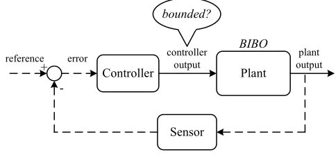
Many engineering systems are BIBO stable due to their inherent dissipative structure. In the ideal case, simple open-loop control strategies that generate a bounded control output can regulate the system output to its desired value without affecting the system stability. However, in a real environment, there are external disturbances and parameter variations that could considerably degrade the system performance. As a result, it is essential to close the loop by using feedback control, as shown in Fig. 1, in order to achieve desired performance, e.g. zero steady-state error, even when there are disturbances, parameter variations and uncertainties. The problem is that a feedback controller no longer guarantees

a bounded control output, which may cause instability. In other words, the stability of the system is no longer preserved. Developing feedback control strategies that preserve the BIBO stability of the system is of significance.

Plant Controller

Sensor

BIBO

plant output controller

output error

reference

+

[image:3.612.315.557.118.233.2]

-bounded?

Figure 1. Closing the loop

Particularly, when a regulation problem is considered, which is the most common control objective, an IC is used to achieve zero steady-state error. Consider a general non-linear system

˙

x=f(x, u), (1)

where f : D ×Du → Rn is locally Lipschitz in x and

u and D, Du are open neighbourhoods of the origin for x

and u, respectively. For simplicity, consider a single-input system in the form of (1) and assume that the control task is the regulation of a scalar function g(x) to zero. This assumption also includes the common regulation scenario of a state variablexito a desired levelxrefi , i.e.g(x) =x

ref i −xi.

The traditional IC that achieves this task is given as

u(t) = ∫ t

0

kIg(x(τ))dτ, (2)

where kI > 0 represents the integral gain. Then, the IC

introduces a dynamic controller that can be written as

u = w (3)

˙

w = kIg(x). (4)

However, closed-loop system stability is not always guaranteed even if the plant (1) is BIBO. Note that for a non-linear system, the BIBO or input-to-output stability is guaranteed if the plant is input-to-state stable (ISS) and the output function isK₋bounded [17]. A generic controller that guarantees the stability of the closed-loop system will be developed in this paper.

III. MAIN RESULT

In this section, the main task is to design a controller that operates similarly to the traditional IC (3)-(4) and generates a bounded output. This controller is calledBounded Integral Controller (BIC) and introduces a second controller state as shown below:

u=w (5)

[

˙ w ˙ wq

]

=



  

−k

(

w2 u2_max+

(wq−b)2 ϵ2 −1

)

kIg(x)c

− ϵ 2

u2_maxkIg(x)c −kq

(

w2 u2_max+

(wq−b)2 ϵ2 −1

) 

   [

w wq

]

(4)

wherewandwq are the controller state variables, bis a

non-negative constant andumax, k,kq,ϵ,care positive constants.

Consider, now, the plant system dynamics

˙

x=f(x, u, u1) (7)

where u describes the control input and u1 is a vector of external uncontrolled inputs.

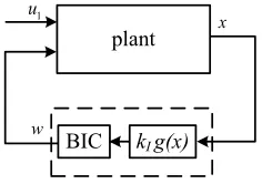
After applying the BIC into the general plant, the closed-loop system is described in Fig. 2, which is a composite feedback interconnection form. Here, it is assumed that the function g(x) is locally Lipschitz, which is true in most control applications. Additionally, the plant system is assumed to possess the ISpS (or ISS) property which holds for most engineering systems. Then, the following theorem guarantees the ISpS property of the closed-loop system.

x

w

1

u

plant

kI g(x)

[image:4.612.116.234.250.333.2]

BIC

Figure 2. Closed-loop system with BIC

Theorem 1. The feedback interconnection of plant system(7) with the proposed BIC(5)-(6)is ISpS with respect to inputu1, when the plant system (7) is ISpS with respect to both inputs

uand u1.

Proof: For the controller dynamics (6), consider the following Lyapunov function candidate

V = w

2 u2 max +w 2 q

ϵ2. (8)

Taking the time derivative ofV, it yields

˙

V = 2ww˙ u2

max

+2wqw˙q ϵ2

=−2

( w2 u2

max

+(wq−b)

2

ϵ2 −1

) (

k w

2

u2

max

+kq

w2 q ϵ2 ) . (9) Its sign is related to an ellipse at the point (0, b)defined by

C=

{

w, wq ∈R:

w2 u2

max

+(wq−b) 2

ϵ2 = 1

}

. (10)

The derivative of the Lyapunov functionV˙ is negative outside of the ellipse C and positive inside of the ellipse except from the origin where it is zero. Note that the Lyapunov function is defined as an ellipsoid structure around the origin, while C represents a given ellipse around (0, b). Defining

Bc=

{

w2 u2_max+

(wq−b)2

ϵ2 ≤(1 +δ)

2}

,whereδis an arbitrary positive constant, from (9) it is holds thatV <˙ 0 outside and on the boundary ofBc except from the origin. Consider now a

closed set Ωs={V(w, wq)≤s}. One can find the value ofs

such thatBc⊆Ωsand the boundaries ofBc andΩsintersect

at point (0, b+ϵ(1 +δ)), as shown in Fig. 3, i.e. this point should satisfy w2 u2 max +w 2 q

ϵ2 =s. (11)

Therefores= (b+ϵ(1+_ϵ2 δ))2 and

S=     

w, wq∈R:

w2 (₍_b₊_ϵ₍₁₊_δ₎₎_u

max ϵ

)2+

w2

q

(b+ϵ(1 +δ))2= 1      (12) describes the boundary ofΩs. Hence, V <˙ 0 outside and on

the boundary ofΩs, which guarantees that the controller states

wandwq introduce an ultimate bound. As a result, it is proven

that for any initial conditionsw(0) andwq(0), there exists a

classKLfunctionβ and a future time instantT ≥0such that [1] w wq ≤ β ( w(0) wq(0)

, t )

, t≤T (13)

and w wq ≤

(umax+ϵ) (b+ϵ(1 +δ))

ϵ , t≥T. (14)

Inequality (14) results from the norm properties

(

∥x_∥_p_{≤ ∥}x_∥₁,_∀p_≥1) and taking into account from (12) that for all t ≥ T, i.e. after the time instant that w and wq enter ellipse S, it holds true that

|w_{| ≤} (b+ϵ(1+δ))umax

ϵ and |wq| ≤ b + ϵ(1 +δ) which

yield that w wq 1

≤ (umax+ϵ)(b+ϵ(1+δ))

ϵ .

Hence, the control states solution can be written in the form:

w wq ≤ β ( w(0) wq(0)

, t )

+d (15)

where d = (umax+ϵ)(b+ϵ(1+δ))

ϵ is a positive constant. Since

inequality (15) is satisfied independently from any bounded inputg(x)of the controller, the controller states can be written in the general ISpS form

w wq ≤

β(∥x(0)∥, t)+γcontrol

( sup 0≤τ≤t∥

kIg(x(τ))∥

)

+d

(16) with zero gain, i.e.γcontrol= 0, regardless of the selection of

the initial conditionsw0,wq0and the parametersk,kq,umax,

b andϵ.

Since the closed-loop system, as shown in Fig. 2, is given in the composite feedback interconnection form, the small-gain theorem given in [19], [20] can be applied. Particularly, given that the controller gain is zero, then the small-gain condition is obviously satisfied. Therefore, the closed-loop system is ISpS with respect to the external input vectoru1.

The special structure of the BIC provides the opportunity of proving the ISpS property for a wide class of non-linear systems. It is obvious that if the external input u1 of the plant is zero, the closed-loop system solution is bounded. It is also worth noting that Theorem 1 holds independently from the plant structure, the controller parametersb_≥0 and

(5)

Ο

w

q

w

S

u

max

(1

+δ

)

(0,

b+ε

(1

+δ

))

B

c

[image:5.612.64.285.56.166.2]

Ω

s

Figure 3. Boundedness of stateswandw_q

Hence, BIC provides a generic controller for non-linear ISpS systems where the plant dynamics and parameters may be unknown or change during the operation.

IV. BICWITH A GIVEN OUTPUT BOUND

A. Controller design

Although the BIC output is proven to remain bounded, a given bound is not guaranteed in general. In order for the con-trol signal to remain inside a given boundu_∈[−umax, umax],

where umax denotes the maximum absolute value of the

controller output, the BIC parameters can be selected as

b= 0, ϵ= 1, c= wqu 2

max

u2

max−u2c

, k= 0, kq >0, (17)

where uc ∈ (−umax, umax) is constant. According to this

selection, the BIC dynamics (6) become

[ ˙ w ˙ wq

] =





0 kIg(x)wqu

2 max u2

max−u2c −kIg(x)_u2 wq

max−u2c −kq

(

w2 u2

max +w

2

q−1

) 

 [

w wq

]

(18) where the initial conditions are chosen w0= 0 (initial condi-tion of the IC, usually zero) and wq0 = 1. Now, considering

the Lyapunov function candidate

W = w

2

u2

max

+wq2, (19)

its derivative yields

˙

W =−2

( _w2

u2

max

+w2q−1

)

kqw2q (20)

which implies that the BIC states are on the ellipse

W0=

{

w, wq ∈R:

w2 u2

max

+wq2= 1

}

(21)

as shown in Fig. 4. This is due to the fact that the initial conditions are defined on W0, where obviously

˙

W = 0⇒W(t) =W(0) = 1, ∀t≥0 (22)

proving that the BIC states will start and remain at all times on the ellipse W0, i.e. the diagonal term −kq

(

w2 u2

max +w

2

q −1

)

will be zero. This term is only used to increase the robustness with respect to external disturbances or calculation errors in the dynamics of wq during a practical implementation. Note

that the same analysis holds for any initial conditions with

wq0>0 andw0 defined on W0.

By considering the following transformation

w=umaxsinθ

wq=cosθ, (23)

it yields from the BIC dynamics (18) that

˙

θ=kIg(x)wqumax u2

max−u2c

(24)

which proves that w and wq will move on the ellipse W0

with angular velocity θ˙ (Fig. 4). Therefore, it is guaranteed that u ∈ [−umax, umax] for all t ≥ 0 and as a result it

extends the BIC operation to guarantee stability for locally ISpS systems. It should be noted that due to the selection of the initial conditions, the desired operation of the controller states on the ellipse is guaranteed even if k = 0 and c is varying such as in the present case. If it is assumed that there exists a desired equilibrium pointx=xe for the plant

with u = ue ∈ (−umax, umax), for which g(xe) = 0, this

implies that w and wq can stop at the desired equilibrium,

corresponding to (ue, wqe)onw−wq plane, at which

˙

θ= kIg(xe)wqeumax u2

max−u2c

= 0.

The conditions under which a possible convergence to the de-sired equilibrium exists are investigated in the next subsection.

Ο 1

W0

wq

w

umax

ue

wqe

[image:5.612.371.504.397.477.2]

θɺ

Figure 4. BIC states onw₋w_qplane

B. Achieving boundedness while preserving the stability of the system with the traditional IC

Consider the non-linear ISpS system of the form of (1) with the proposed BIC with the given bound (18). Since no other external inputs are present, the closed-loop system solution

xBIC(t) will be bounded, wherexBIC =[ xT w wq ] T

is the state vector of the closed-loop system. However, since in this note the BIC is used to perform similarly to the traditional IC for achieving a desired regulation scenario, it is important to prove that the BIC does not change the behaviour of the IC near the desired equilibrium point.

Consider an ISpS plant controlled by the traditional IC (1), (3), (4). In this case assume that bothf andgare continuously differentiable functions. The closed-loop system can be written in the form

˙

xIC=fIC(xIC) (25)

where xIC = [ xT w ] T

is the state vector. Assume that

xICe=

[ xT

e we ]

T

(6)

0. If linearisation around the equilibrium point results in a Jacobian matrix AIC = ∂fIC_∂x(_ICxIC)

xIC=xICe

withReλi <0

for all eigenvalues of AIC, then the equilibrium point of (25)

will be asymptotically stable. However, it is not guaranteed that the solution of the closed-loop system will not escape to infinity, e.g. if initial conditions are defined away from the equilibrium point.

As it is shown in the sequel, the BIC maintains the asymp-totic stability of the equilibrium point and according to the previous analysis, the proposed control method additionally guarantees a maximum bound for the closed-loop solution and a given bound for the controller output, leading to a superior performance and more rigorous theoretical analysis compared to the traditional IC.

In this framework, consider the following conditions: 1) xICe = [ xTe we ]

T

is an equilibrium point of (25) withwe∈(−umax, umax).

2) Reλi <0 for all eigenvalues of AIC and for any 0<

kI < kImax.

3) The BIC parameteruc satisfies

−umax

√

1− kI

kImax

< uc< umax

√

1− kI

kImax

.

(26) Then the following proposition can be formulated:

Proposition 2. If Conditions 1)-3) above are satisfied, then the closed-loop system resulting from the feedback intercon-nection of the ISpS plant (1) and the BIC (5), (18) has an asymptotically stable equilibrium point [

xT

e we wqe ]

T

withwqe=±

√

1− w2e

u2 max.

Proof: Based on the analysis of the previous subsection, the equilibrium point xICe =

[ xT

e we ]

T

of (25), where

we∈(−umax, umax), will correspond to an equilibrium point

xBICe=[ xTe we wqe ]

T

of the feedback interconnection of the ISpS plant (1) and the BIC (5), (18), where wqe =

±√1− w2e u2

max for which0< w

2

qe≤1, since it is defined on

W0withwe∈(−umax, umax). According to Condition 2) all

eigenvalues of

AIC=

   ∂f ∂x

(xe,we) ∂f ∂w

(xe,we)

kI∂g_∂x

₍_x

e,we)

0 

 

have negative real parts for any 0 < kI < kImax.

In the same framework, linearisation around xBICe =

[

xTe we wqe ]

T

for the closed-loop system with the BIC results in the Jacobian

ABIC=

      ∂f ∂x ₍

xe,we)

∂f ∂w

₍

xe,we)

0n×1

kI∂g_∂x

(xe,we) w2

qeu2max u2

max−u2c 0 0 −kI_∂x∂g

₍_x

e,we) wewqe u2_max−u2_c −2

kqwewqe

u2_max −2kqw

2 qe       ,

where wqe ̸= 0 sincewe∈ (−umax, umax) andwe andwqe

are defined on W0. Since−2kqw2qe<0, then all eigenvalues

of ABIC will have negative real parts if matrix

ABIC1=

   ∂f ∂x ₍

xe,we)

∂f ∂w

₍

xe,we)

kI∂g_∂x

(xe,we) w2

qeu2max u2

max−u2c 0



 

is Hurwitz. Since 0< w2

qe≤1, then

0 < kI

w2

qeu2max

u2

max−u2c

≤kI

u2_max u2

max−u2c

,

⇒0 < kI

w2

qeu2max

u2

max−u2c

< kImax

taking into account (26) from Condition 3). Therefore, all eigenvalues of ABIC1 have negative real parts since the

eigenvalues ofAIC are located at the left half plane for any

0 < kI < kImax. As a result, the equilibrium point of the

closed-loop system with the BIC is asymptotically stable. It should be noted that if Condition 2) is satisfied for anykI >0,

then the desired equilibrium of the closed-loop system with the BIC is asymptotically stable for anyuc∈(−umax, umax).

Furthermore, even if the control output tries to reach the limits during transients, i.e.u_{→ ±}umax, thenwq →0and the

first equation of (18) results inw˙ _→0independently from the functiong(x). This means that the integration slows down near the limits preventing an integration windup problem. Opposed to the traditional anti-windup structures, the BIC does no stop the integration but smoothly slows it down near the limits without additional switches; hence the plant input remains a continuous-time signal, which proves the closed-loop system stability. Additionally,wandwq stay exclusively in the first 2

quadrants in Fig. 4 for initial conditions defined on the upper semi-ellipse of W0, and therefore they cannot move around

W0, which excludes an oscillating behaviour of the controller state dynamics around the ellipse.

The closed-loop system stability in the sense of bounded-ness and the given bound for the controller output have been proven in this note independently from the existence of an equilibrium point or its stability properties (stable or unstable). Therefore, if the equilibrium point changes from a stable to an unstable mode (eg. change of gain kI) or is shifted

outside the bounded range, closed-loop stability in the sense of boundedness is still maintained, opposed to the traditional IC or the IC with a saturation unit.

V. PRACTICAL EXAMPLE

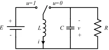
In order to verify the proposed BIC in comparison to the traditional IC, the dc/dc buck-boost converter, shown in Fig. 5, is simulated. This power converter system is widely used in power applications (photovoltaic, energy storage systems, etc.) since it can regulate the dc output voltage to a higher or lower level than the dc input voltage by suitably controlling the switching element of the device.

(7)

E +

-L C R

+

-v

i

[image:7.612.86.267.56.139.2]

u=1 u=0

Figure 5. The dc/dc buck-boost converter

given as

Ldi

dt = −(1−u)v+uE (27)

Cdv

dt = (1−u)i−

v

R, (28)

whereLandCare the converter inductance and capacitance, respectively, R is the load resistor and E is the dc input voltage. The system states are the inductor current iand the capacitor voltage v, while the control input is the duty-ratio

u, which is a continuous-time signal in the range [0,1]. It should be noted that the system states are bounded for any

u_∈[0,1−γ],where0< γ_≤1, while the upper limit of the inputu= 1 leads the inductor current to instability.

The main task is to regulate the output voltagev to a given dc reference value vref. Although several control schemes

have been developed in the literature, such as traditional or cascaded PI controllers [30], passivity-based controllers [29], etc., in the industry, traditional or cascaded PI controllers are commonly used due to their simple structure and implementa-tion. This is also due to the fact that the system dynamics can change (e.g. if a complicated load is added in the output) and the system parameters can be unknown or change during the operation. Even though, in these cases, stability may not be guaranteed, traditional controllers are still used for simplicity and are usually tuned in an empirical manner.

In this example, a traditional voltage IC with g(x) = vref −v is investigated and compared with the BIC with

a given bound. The system parameters are L = 10mH,

C = 30µF, R = 15Ω andE = 15V. Initially the reference

output voltage is set to vref = 30V. For stability reasons,

in practice, it is often required the duty-ratio uto be limited below 1, usually 0.8 (i.e., γ = 0.2) to avoid a high inductor current. Since the BIC maintains the controller output in the range[−umax, umax], one can setu=w2 andumax=

√

0.8. In this way the required range[0,0.8]for the control output can be achieved with the BIC. If the closed-loop system with the corresponding IC is linearised around the desired equilibrium point, it can be obtained (e.g. using root locus) that the equilibrium is asymptotically stable for all 0 < kI < kImax,

where kImax ≈ 1. Thus, the integral gain can be chosen

kI = 0.2 for both the IC and the BIC, where additionally

two different choices of uc are tested uc =

√

0.65 ≈ 0.8

anduc=

√

0.5≈0.7that satisfy (26). Note that if the system parameters are unknown in practice,kI andkImaxare usually

chosen based on experience and observation.

The converter is simulated with the traditional IC and the IC with a saturation unit in the output at[0,0.8], and is compared

to the BIC with two different values ofuc. Starting with zero

initial conditions for the system states and the control output, the output voltage reference is set tovref = 30V att= 0.5s.

At time instant t = 1s,vref suddenly increases to 70V and

drops back to 30V att = 2s. Finally, at t = 3s, vref is set

to 50V. The time response of the system is shown in Fig. 6. Initially, both the IC with and without the saturation unit and the BIC regulate the output voltage at the desired level. However, when vref is set to 70V, the traditional IC leads

the inductor current to instability. The duty-ratio of the IC with the saturation unit saturates at the upper limit 0.8, while the BIC with either selection ofuc smoothly converges to the

upper limit. In this case, the desired equilibrium is shifted outside the bounded range and the IC with the saturation suffers from integrator windup, opposed to the BIC which automatically slows down the integration. This is observed when vref changes back to 30V and the IC with saturation

results in a larger transient. Finally, when vref is set to 50V,

the BIC converges to the desired equilibrium while the IC with saturation suffers again from integrator windup and results in an oscillatory response. Note that the different choice of uc

in the BIC design will result into slightly different transient response, since this parameter affects the angular velocity (24) of the BIC states on the desired ellipseW0. The operation on the ellipse is illustrated in Fig. 7, where it is clear that the controller states remain on the upper semi-ellipse of W0 as required.

It should be underlined that if the system parameters are completely unknown or change during the system operation, neither the IC or the BIC can guarantee asymptotic stability of the desired equilibrium. However, the BIC can still guarantee an ultimate bound for the closed-loop system, a given bound for the control output and the fact that it will not suffer from integrator windup issues. This is the main result of the current note which offers a replacement of the traditional IC with the BIC and can be applied in many engineering systems where the IC is used without a rigorous proof of stability.

VI. CONCLUSIONS

(8)

IC with and without saturation BIC

0 1 2 3 4

0 10 20 30 40 50 60 70 80

Time/s

v/V

IC IC+sat

0 1 2 3 4 0

10 20 30 40 50 60 70 80

Time/s

v/V

BIC (u_c=0.8) BIC (u_c=0.7)

(a) output voltagev

0 1 2 3 4 0

5 10 15 20 25

Time/s

i/A

IC IC+sat

0 1 2 3 4 0

5 10 15 20 25

Time/s

i/A

BIC (u_c=0.8) BIC (u_c=0.7)

(b) inductor currenti

0 1 2 3 4 0

0.2 0.4 0.6 0.8 1

Time/s

u

IC IC+sat

0 1 2 3 4 0

0.2 0.4 0.6 0.8 1

Time/s

u

BIC (u_c=0.8) BIC (uc=0.7)

[image:8.612.51.296.55.394.2]

(c) duty-ratiou

Figure 6. Simulation results of the buck-boost converter with the IC and the BIC

−1 −0.5 0 0.5 1

wq

w W

[image:8.612.97.242.438.552.2]

0

Figure 7. w₋w_q plane for the BIC

REFERENCES

[1] H. K. Khalil,Nonlinear Systems. Prentice Hall, 2001.

[2] Q.-C. Zhong and T. Hornik,Control of Power Inverters in Renewable Energy and Smart Grid Integration. Wiley-IEEE Press, 2013. [3] M. Corless and G. Leitmann, “Continuous state feedback guaranteeing

uniform ultimate boundedness for uncertain dynamic systems,”IEEE Trans. Autom. Control, vol. 26, no. 5, pp. 1139–1144, 1981.

[4] J. Tsinias, “Sufficient Lyapunov-like conditions for stabilization,” Math-ematics of control, Signals and Systems, vol. 2, no. 4, pp. 343–357, 1989. [5] M. Morari, “Robust stability of systems with integral control,” IEEE

Trans. Autom. Control, vol. 30, no. 6, pp. 574–577, 1985.

[6] T. Fliegner, H. Logemann, and E. P. Ryan, “Low-gain integral control of continuous-time linear systems subject to input and output nonlinear-ities,”Automatica, vol. 39, no. 3, pp. 455–462, 2003.

[7] D. Mustafa, “How much integral action can a control system tolerate?” Linear algebra and its applications, vol. 205, pp. 965–970, 1994. [8] A. Isidori and C. I. Byrnes, “Output regulation of nonlinear systems,”

IEEE Trans. Autom. Control, vol. 35, no. 2, pp. 131–140, 1990. [9] J. Huang and W. J. Rugh, “On a nonlinear multivariable servomechanism

problem,”Automatica, vol. 26, no. 6, pp. 963–972, 1990.

[10] N. A. Mahmoud and H. K. Khalil, “Asymptotic regulation of minimum phase nonlinear systems using output feedback,”IEEE Trans. Autom. Control, vol. 41, no. 10, pp. 1402–1412, 1996.

[11] A. Isidori, “A remark on the problem of semiglobal nonlinear output regulation,” IEEE Trans. Autom. Control, vol. 42, no. 12, pp. 1734– 1738, 1997.

[12] H. K. Khalil, “Universal integral controllers for minimum-phase nonlin-ear systems,”IEEE Trans. Autom. Control, vol. 45, no. 3, pp. 490–494, 2000.

[13] C. I. Byrnes and A. Isidori, “Asymptotic stabilization of minimum phase nonlinear systems,”IEEE Trans. Autom. Control, vol. 36, no. 10, pp. 1122–1137, 1991.

[14] Z.-P. Jiang and I. Mareels, “Robust nonlinear integral control,” IEEE Trans. Autom. Control, vol. 46, no. 8, pp. 1336–1342, 2001.

[15] A. Singh and H. K. Khalil, “State feedback regulation of nonlinear systems using conditional integrators,” in 43rd IEEE Conference on Decision and Control (CDC), vol. 5. IEEE, 2004, pp. 4560–4564. [16] R. Li and H. K. Khalil, “Conditional integrator for non-minimum phase

nonlinear systems,” in51st IEEE Conference on Decision and Control (CDC), 2012, pp. 4883–4887.

[17] E. D. Sontag, “Smooth stabilization implies coprime factorization,”IEEE Trans. Autom. Control, vol. 34, no. 4, pp. 435–443, 1989.

[18] E. D. Sontag and Y. Wang, “New characterizations of input-to-state stability,”IEEE Trans. Autom. Control, vol. 41, no. 9, pp. 1283–1294, 1996.

[19] Z.-P. Jiang, A. R. Teel, and L. Praly, “Small-gain theorem for ISS systems and applications,”Mathematics of Control, Signals and Systems, vol. 7, no. 2, pp. 95–120, 1994.

[20] Z.-P. Jiang and I. M. Y. Mareels, “A small-gain control method for nonlinear cascaded systems with dynamic uncertainties,”IEEE Trans. Autom. Control, vol. 42, no. 3, pp. 292–308, 1997.

[21] A. R. Teel, “A nonlinear small gain theorem for the analysis of control systems with saturation,”IEEE Trans. Autom. Control, vol. 41, no. 9, pp. 1256–1270, 1996.

[22] A. Donaire and S. Junco, “On the addition of integral action to port-controlled Hamiltonian systems,”Automatica, vol. 45, no. 8, pp. 1910– 1916, 2009.

[23] R. Ortega and J. G. Romero, “Robust integral control of port-Hamiltonian systems: The case of non-passive outputs with unmatched disturbances,” Systems & Control Letters, vol. 61, no. 1, pp. 11–17, 2012.

[24] L. Zaccarian and A. R. Teel, “Nonlinear scheduled anti-windup design for linear systems,”IEEE Trans. Autom. Control, vol. 49, no. 11, pp. 2055–2061, 2004.

[25] S. Galeani, S. Onori, and L. Zaccarian, “Nonlinear scheduled control for linear systems subject to saturation with application to anti-windup control,” in46th IEEE Conference on Decision and Control, 2007, pp. 1168–1173.

[26] Y. Peng, D. Vrancic, and R. Hanus, “Anti-windup, bumpless, and conditioned transfer techniques for PID controllers,”IEEE Control Syst. Mag., vol. 16, no. 4, pp. 48–57, 1996.

[27] C. Bohn and D. P. Atherton, “An analysis package comparing PID anti-windup strategies,”IEEE Control Syst. Mag., vol. 15, no. 2, pp. 34–40, 1995.

[28] S. Tarbouriech and M. Turner, “Anti-windup design: an overview of some recent advances and open problems,” IET Control Theory & Applications, vol. 3, no. 1, pp. 1–19, 2009.