Verification of BOUT++ by the method of manufactured solutions

This is a repository copy of

Verification of BOUT++ by the method of manufactured

solutions

.

White Rose Research Online URL for this paper:

http://eprints.whiterose.ac.uk/101319/

Version: Published Version

Article:

Dudson, Benjamin Daniel orcid.org/0000-0002-0094-4867, Madsen, Jens, Omotani, John

Tomotaro et al. (3 more authors) (2016) Verification of BOUT++ by the method of

manufactured solutions. Physics of Plasmas. 062303. ISSN 1089-7674

https://doi.org/10.1063/1.4953429

[email protected] https://eprints.whiterose.ac.uk/ Reuse

Items deposited in White Rose Research Online are protected by copyright, with all rights reserved unless indicated otherwise. They may be downloaded and/or printed for private study, or other acts as permitted by national copyright laws. The publisher or other rights holders may allow further reproduction and re-use of the full text version. This is indicated by the licence information on the White Rose Research Online record for the item.

Takedown

If you consider content in White Rose Research Online to be in breach of UK law, please notify us by

Verification of BOUT++ by the method of manufactured solutions

B. D. Dudson, J. Madsen, J. Omotani, P. Hill, L. Easy, and M. Løiten

Citation: Physics of Plasmas 23, 062303 (2016); doi: 10.1063/1.4953429 View online: http://dx.doi.org/10.1063/1.4953429

View Table of Contents: http://scitation.aip.org/content/aip/journal/pop/23/6?ver=pdfcov Published by the AIP Publishing

Articles you may be interested in

Strong anisotropy in quasi-static magnetohydrodynamic turbulence for high interaction parameters Phys. Fluids 26, 025109 (2014); 10.1063/1.4864654

Alfvén wave collisions, the fundamental building block of plasma turbulence. II. Numerical solution Phys. Plasmas 20, 072303 (2013); 10.1063/1.4812807

Interaction of a thin shock with turbulence. I. Effect on shock structure: Analytic model Phys. Fluids 20, 127102 (2008); 10.1063/1.3041706

Anomalous cross field electron transport in a Hall effect thruster Appl. Phys. Lett. 89, 161503 (2006); 10.1063/1.2360182

Verification of BOUT

₁₁

by the method of manufactured solutions

1_{York Plasma Institute, Department of Physics, University of York, Heslington, York YO10 5DD,}

United Kingdom

2_{Department of Physics, Technical University of Denmark, DK-2800 Kgs. Lyngby, Denmark}

3_{Department of Physics, Chalmers University of Technology, SE-412 96 G} €

oteborg, Sweden 4_{CCFE, Culham Science Centre, Abingdon OX14 3DB, United Kingdom}

(Received 18 March 2016; accepted 23 May 2016; published online 9 June 2016)

BOUTþþ is a software package designed for solving plasma fluid models. It has been used to

simulate a wide range of plasma phenomena ranging from linear stability analysis to 3D plasma turbulence and is capable of simulating a wide range of drift-reduced plasma fluid and gyro-fluid models. A verification exercise has been performed as part of a EUROfusion Enabling Research project, to rigorously test the correctness of the algorithms implemented in BOUTþþ, by testing order-of-accuracy convergence rates using the Method of Manufactured Solutions (MMS). We present tests of individual components including time-integration and advection schemes, non-orthogonal toroidal field-aligned coordinate systems and the shifted metric procedure which is used to handle highly sheared grids. The flux coordinate independent approach to differencing along

magnetic field-lines has been implemented in BOUTþþand is here verified using the MMS in a

sheared slab configuration. Finally, we show tests of three complete models: 2-field Hasegawa-Wakatani in 2D slab, 3-field reduced magnetohydrodynamics (MHD) in 3D field-aligned toroidal coordinates, and 5-field reduced MHD in slab geometry. [http://dx.doi.org/10.1063/1.4953429]

I. INTRODUCTION

The BOUTþþcode1,2is an open source toolkit for the simulation of plasma models. Its applications include the study of plasma transients including edge localised modes and filament/blob transport, and turbulence in magnetised plasma devices. Here, we present a rigorous code verification exercise3,4of the BOUTþþcore algorithms and numerical methods using the Method of Manufactured Solutions (MMS).3,5Code verification is a process of checking that the chosen set of partial differential equations is solved correctly and consistently and is a purely mathematical exercise. Code verification is not concerned with verifying that the chosen numerical methods are appropriate for the chosen set of equations. Code verification is also not concerned with test-ing the ability of a given model to explain experimental observations. This testing is dealt with in the subsequent validation process. Code verification tests typically rely on a known solution against which to check the result (the Method of Exact Solutions). In relatively simple geometries (e.g., slabs or cylinders) and equations (usually linearised), an analytical solution can sometimes be found, and this kind of test is used to verify BOUT6and BOUTþþ1

as part of a test suite, run regularly to reduce the chances of errors being introduced. The requirement that there be an analytical solu-tion restricts the usefulness of the tests, as the code cannot be verified for realistic geometries and problems of interest, where no such exact solution exists.

The Method of Manufactured Solutions (MMS)3,5

pro-vide a method by which a simulation code can be verified in general situations, even where analytic solutions cannot be found. This is done by imposing a known “manufactured”

solution, and adding sources to the equations such that the manufactured solution is an exact solution to the modified set of equations. The manufactured solution and therefore also the source can be composed of primitive analytical func-tions sin;cos;tanh, etc., which can be evaluated with a very high accuracy, typically double floating point precision. The difference between the numerically calculated solution and the “exact” manufactured solution provides the numerical error. The scaling of the numerical error with the numerical spatial resolution is knowna priori, and hence any deviation from the theoretical scaling must be due to code inconsisten-cies or errors. The MMS is a very general technique, which has been used to verify a wide range of engineering codes,

particularly in the fluid dynamics community.7 MMS has

been applied to components of plasma simulation codes such as the European Transport Solver8 and gyrokinetic simula-tions,9and has recently been applied to the GBS turbulence code10and tokamak edge simulations.11

As in Ref.10, here we focus on order-of-accuracy tests as they provide the most rigorous test of numerical imple-mentation.4 In Section II, we describe in more detail the

MMS procedure, and the changes made to BOUTþþ to

facilitate its routine use. BOUTþþ simulations typically employ non-orthogonal curvilinear coordinate systems,

which are described in Section III along with the method

used to perform tests in these coordinates. Individual compo-nents of BOUTþþare first tested independently, including time integration schemes in SectionIV A, advection schemes in SectionIV B, and operators for wave and diffusion equa-tions along magnetic fields in SectionIV C. Coordinate sys-tems are then tested in SectionIV E. In SectionV, complete models are tested, in which these components are combined: The 2-field Hasegawa-Wakatani model of drift-wave turbu-lence in SectionV A; a 3-field reduced Magnetohydrodynamics

a)

Electronic mail: [email protected]

1070-664X/2016/23(6)/062303/12/$30.00 23, 062303-1

(MHD) model in Section V B; and a 5-field reduced MHD model similar to that in Ref.10is tested in SectionV C.

All source code, input files, and scripts needed to pro-duce the figures and results in this paper are publicly

avail-able as part of the BOUTþþ development repository at

https://github.com/boutproject/BOUT-dev, revision 83c1f53. Due to automation of the testing procedure (SectionII), most results and figures in this paper can be reproduced by run-ning a single Python script. The location of these scripts will be specified relative to the root of the git repository.

II. TESTING FRAMEWORK

The BOUTþþ code is not limited to a single set of

equations, but has been developed to allow an arbitrary num-ber of evolving fields, and input of custom evolution equa-tions in a form close to mathematical notation (see Refs. 1 and 2 for details). This flexibility presents a challenge for verification, due to the large number of possible combina-tions of operators and settings such as boundary condicombina-tions, which could be employed. Fortunately, as pointed out in Ref. 5, only mutually exclusive settings and operators need be in-dependently tested, not all possible combinations of options. This still requires a relatively large number of tests to adequately cover the code components, and to verify each model. The process of MMS testing has therefore been auto-mated as far as possible, by enabling all aspects of the test to be specified in an input text file. This allows the same code to be tested with different inputs, and new tests to be created more easily. Here, we briefly outline the MMS procedure,

before describing the mechanisms implemented in

BOUTþþto carry out MMS testing.

Time integration codes such as BOUTþþ evolve a set

of nonlinear equations for quantities f, e.g., for a two field model evolving particle density and temperaturef ¼ fn;Tg. The system of equations is solved using the method of lines and can be written in a general form as

@f

@t ¼F f ; (1)

where FðÞ is a nonlinear operator which contains discre-tised differential operators in the spatial dimensions. In order to test the correctness of the numerical implementa-tion, a time-dependent functionfMðtÞis chosen (manufac-tured) using a combination of primitive mathematical functions which can be evaluated to machine precision. Manufactured solutions should be chosen so that they exer-cise all parts of the code, so should be varying in time and all spatial dimensions. Ideally the magnitude of the terms in the equations solved should be comparable, so that the error in one does not dominate over the others. Since derivatives of the solution will be taken numerically, the solution should also be smooth. Where the domain is periodic, such as toroidal angle in tokamak simulations, the manufactured solutions must also be periodic in those directions. A detailed discussion of selection criteria for manufactured solutions can be found in Ref.5.

The manufactured function fM is now inserted into the

function FðÞ and @f

M

@t to calculate a source function S

analytically

S tð Þ ¼@f M

@t F f M

: (2)

The functionFðÞis typically composed of a combination of algebraic operations and differential operators. This results in a closed analytic form forFðfMÞeven whenFðÞis nonlin-ear or evaluated in non-orthogonal curvilinnonlin-ear coordinate systems, since fM is only ever differentiated with respect to time and spatial coordinates, and not integrated. In some cases FðÞ contains integrals, as in the models tested in SectionV, where the potential/is calculated by integrating the vorticity. These integrals may not have a closed analytic solution, and so in these cases a solution to the integral (potential /) is manufactured, and a source then calculated to be added to the integrand (vorticity).

Here, the symbolic packages Mathematica and the Sympy library12 were used to calculate source functions. Both can generate representations of the resulting expres-sions which can be copied directly into source code or text input files. For large sets of equations such as those in Section V C, this is essential in order to avoid introducing errors.

The system of equations to be solved numerically is now modified to

@f

@t¼F f þS tð Þ (3)

so that the functionfMis an exact (manufactured) solution of Equation(3). SinceShas been calculated analytically, it can be evaluated to within machine precision at any desired time, and passed to the time integration routines. At the start of the simulation t¼0, the state is set to the manufactured

solution f ¼fMðt¼0Þ. The simulation time is then

advanced to some later time t¼Dt, at which point the nu-merical solutionf is compared to the manufactured solution

fM_{ðt¼DtÞ. The norm of the difference between the}

numeri-cal solution and the manufactured solution ¼ jjf fMjjat

t¼Dtthen gives a measure of the error in the numerical so-lution, which should converge towards zero as the spatial and temporal mesh is refined. Note that in order to obtain convergence in the solution of a time-dependent Partial Differential Equation (PDE), both the spatial and temporal mesh (time step) must be refined.13In general, separating the spatial and temporal convergence is non-trivial, but in SectionIV Dwe use a slightly different procedure than out-lined above, to verify spatial convergence and boundary con-ditions independently of temporal convergence.

Boundary conditions must also be modified for testing with the MMS. A Dirichlet boundary condition on a quantity

nðboundaryÞ ¼nMðboundary;tÞ: (4)

Similarly for Neumann boundary conditions

@n

@xðboundaryÞ ¼

@nM

@x ðboundary;tÞ: (5)

More complex boundary conditions such as sheaths, which couple multiple fields together, can be treated by adding a source function as for the time integration equation(3). The boundary conditions applied to all fields now become time-dependent and must be evaluated from an analytic expres-sion at arbitrary points in time.

In order to test a numerical model using the Method of Manufactured Solutions, three analytic function inputs are therefore required for each evolving field (e.g., density n, temperatureT):

(1) A manufactured solution.

(2) A source function calculated from Equation (2)using a symbolic package like SymPy.

(3) Analytic expressions for boundary conditions.

As described in Ref. 2, BOUTþþ contains an

expres-sion parser which evaluates analytic expresexpres-sions in input files. This was added as a convenient means to specify initial conditions but has been extended and adapted for use in MMS testing. Once MMS testing is enabled by setting a flag

in the input, BOUTþþ reads a manufactured solution from

the input for each evolving variable, using it to initialise the variable and to calculate an error at each output time; a source function is read and used to modify the time deriva-tives which are passed to the time-integration code; and expressions for boundary conditions are evaluated at the required times. All of this machinery is independent of the specific model, and in most cases, does not require any modi-fication of the problem-specific code. (The only code changes required for MMS testing are Laplacian inversions, which currently require some modifications to their calls in order to insert additional source functions.) The form of the analytic expressions is of course problem specific, but once

calculated, a BOUTþþexecutable can be tested using MMS

and then used to perform physics simulations without recompiling, only changing the input file. This automation of the testing process aims to lower the barriers to routine

test-ing of BOUTþþ simulation models using the Method of

Manufactured Solutions.

III. COORDINATE SYSTEMS

In strongly magnetized plasmas, the characteristic gradi-ent length scales parallel to the magnetic field are often much longer than the perpendicular length scales. This scale separation is often exploited in numerical simulation to reduce the computational cost by using a coarser discretisa-tion in the direcdiscretisa-tion parallel to the magnetic field. A widely used approach is to express the model equations in magnetic field-aligned, curvilinear coordinates. In most previous BOUTþþsimulations,1we have used the so-called balloon-ing coordinates. Startballoon-ing from orthogonal toroidal flux coor-dinates14 ðw;h;fÞ with radial flux-surface labelw, poloidal

angleh, and toroidal anglef, the coordinates are transformed to field-aligned ballooning coordinatesðx;y;zÞ15

x¼w y¼h z¼f

ðh h0

dh ¼ Bfr BhR

; (6)

whereBf andBh are the toroidal and poloidal magnetic field components,ris the minor radius,Ris the major radius, and

is the local magnetic field-line pitch. Moving alongyat fixed

xandzfollows the path of a field-line in bothhandf. The co-variant basis vector (the vector between grid-points) is1

~ex¼ 1 RBh

~_e^wþIR~_{^ef; (7a)}

~ey¼hh Bh

~

B; (7b)

~ez¼R~^ef; (7c)

where~e^are the unit vectors in the original orthogonal toroi-dal ðw;h;fÞcoordinate system, and I¼Ð @

@wdh is the inte-grated shear. The magnetic field is given byB~¼ rz rx, and so the derivative along the magnetic field reduces to a simple partial derivative B~ r ¼ rz rx ry@y. Since

fluctuations typically have long wavelengths along field-lines, a lower resolution can be used in this parallely coordi-nate, with a corresponding reduction in computational resources, both run time and memory.

In order to reduce the deformation of the coordinates caused by magnetic shearI(see~exin Equation(7)), a shifted metric method16,17is usually used, a discussion of which can be found in Ref.1and more recently in Ref.18. At eachy¼

const plane, a local coordinate system is defined in whichx

and zare orthogonal. Mapping between these local coordi-nates and the global field-aligned coordicoordi-nates can be done using Fast Fourier Transforms (FFTs) in the toroidal (f,z) direction. As implemented in BOUTþþ, this procedure has no effect on differencing in the parallel direction, but differ-encing inxis modified by shifting quantities inzusing FFTs before calculating finite differences.

A toroidal coordinate system for MMS testing is gener-ated by first specifying the path of magnetic field lines in poloidal and toroidal angle. The poloidal magnetic field can then be calculated by differentiation, ensuring that the result-ing analytic metric tensor components have relatively com-pact closed forms. The formula used here for the toroidal angle fas a function of the radial (flux) coordinate w and poloidal anglehis

f¼qðwÞ½hþsinh; (8)

whereqðwÞis the safety factor, which is taken to be a para-bolic function ofwvarying between 2 and 3 in SectionsIV E andV B.¼r=R0 is the inverse aspect ratio, here taken to be¼0:1. From this, the field line pitch is calculated as

¼qðwÞ½1þcosh: (9)

A fixed value of the poloidal current function f ¼BfRand minor radiusr¼R0 is used, and the major radius of a field

line varies as R¼R0þrcosh. Equation (9) is then rear-ranged to give an expression for the poloidal field. The inte-grated shear is calculated from the differential of the field-line toroidal anglefwith respect tow

I¼

ðh h0

@ @wdh¼

@qð Þw

@w ½1þcosh: (10)

The resulting covariant and contravariant metric tensors have the same non-zero pattern as in simulations of real devices, and elements of the covariant metric tensor vary in both radial and poloidal coordinates.15 Differencing opera-tors parallel and perpendicular to the magnetic field are tested in this coordinate system in SectionIV E, and a 3-field electromagnetic reduced MHD model is verified in this coor-dinate system in SectionV B.

A. Flux coordinate independent (FCI) scheme

Recently, a new approach to plasma turbulence simula-tions has been developed,18,19and work is ongoing to imple-ment this scheme in several simulation codes. We have implemented this Flux Coordinate Independent (FCI) scheme

in BOUTþþ, enabling the development of complex

turbu-lence models in arbitrary magnetic geometry. By assuming that the poloidal plane equals the plane perpendicular to the magnetic field, complex non-orthogonal curvilinear field-aligned flux coordinates do not need to be used in the perpen-dicular direction, but can use simple geometries (e.g., Cartesian). Here, we verify that these numerical schemes have been implemented correctly for a sheared slab geometry. Further development and verification in more complex geo-metries will be the subject of a future publication.

The flux coordinate independent scheme, as

imple-mented in BOUTþþ, employs 3rd-order Hermite

polyno-mial interpolation in the plane perpendicular to the magnetic field, and 2nd-order central differencing along the magnetic field. The idea is illustrated in Figure 1: The grid is con-structed to be dense in planes perpendicular to the magnetic field and sparse along the magnetic field, since from physical

arguments we expect the solutions to vary slowly along mag-netic field-lines (kjjk?). To calculate derivatives of a

quantity f along magnetic fields, the magnetic field is first followed from each grid point onto neighbouring planes; val-ues of f on neighbouring planes are then interpolated onto these intersection locations. This gives the value of f at 3 points along the magnetic field (the starting grid point, and one point along the field in each direction), which is suffi-cient to calculate second-order accurate first or second deriv-atives using central differencing. If higher order derivderiv-atives are required, then the magnetic field could be followed to calculate intersections with further planes. There are subtle issues with this scheme which will not be addressed here and are left to future work: the treatment of boundary conditions where magnetic field-lines intersect material surfaces, and time-evolving magnetic fields where the mapping of field-lines to neighbouring planes might need to be updated are two areas of interest. The efficiency of the scheme in terms of the computing time required for high-order interpolation is also important in determining the best overall scheme to employ and is also left to future work.

IV. RESULTS

Since operators can be tested and verified independently (see Ref. 5and discussion in SectionII), a suite of smaller tests is generally more useful than a test which combines everything together. Whole models are tested in Section V, but require considerable computing resources to run, and if one of these fails then it is difficult to know where the error lies. Tests of individual components can run in minutes on a desktop, rather than hours on a supercomputer, and a test failure provides better guidance as to the location of the error. The difficulty is in the large number of tests needed to ensure coverage. Here, we verify the major components of

BOUTþþ, including time integration schemes (Section

IV A), advection operators (Section IV B), central schemes for wave and diffusion equations (SectionIV C), and the cur-vilinear coordinate system used for tokamak simulations (Section IV E). Other components, such as calculation of potential/from vorticity, are verified as part of full models (Section V), and development of individual tests for these components is a matter of ongoing work.

A. Time integration

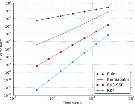
Several explicit and implicit time integration schemes are implemented in BOUTþþ, allowing users to choose at run-time which scheme to use. Methods tested are the Euler, RK4,20a multi-step method derived by Karniadakiset al.21,22

and a third-order Strong Stability Preserving Runge-Kutta method (RK3-SSP).23Results obtained by integrating@f_@t¼f

betweent¼0 andt¼1 are shown in Figure2. Other functions such as @f_@t¼cosðtÞ have also been tested, resulting in the same convergence rate.

The Euler, RK3-SSP, and RK4 methods all reproduce their expected convergence rates (first, third, and fourth order indt, respectively), and so can be considered verified. The Karniadakis scheme is expected to be third order

accurate, but only second order convergence is observed. This is most likely due to the initialisation procedure of the multistep method: At each step, the value of f and its time derivative at two previous timesteps are required, and so to start the simulation these previous steps are constructed using Euler’s method. This results in anOðdt2_Þerror, reduc-ing the overall convergence to second order indt.

Time integration in BOUTþþ simulations is typically

done using implicit adaptive Jacobian-Free Newton Krylov (JFNK) schemes, provided by either the SUite of Nonlinear and Differential/ALgebraic equation Solvers (SUNDIALS24) or the Portable, Extensible Toolkit for Scientific Computation (PETSc25,26). These use adaptive order and adaptive timesteps in order to achieve a user-specified tolerance, and so are diffi-cult to validate using the MMS method. Here, we take as given that the time integration methods in these libraries are implemented correctly and use SUNDIALS for time integra-tion in the remainder of this paper with a relative tolerance of 108and an absolute tolerance of 1012. These small toleran-ces are used so that the spatial discretisation error we are inter-ested in dominates over the time integration error in the results which follow.

B. Advection schemes

A key component of drift-reduced plasma simulations are operators for drifts across magnetic field-lines. These can be written in the form of an advection equation, or as a

Poisson bracket. For example, the EB drift of a scalar

quantityf(e.g., density), due to an electrostatic potential/is

@f

@t ¼

1

Bb~ r/ rf ¼ ½/;f: (11)

Several schemes for calculating the Poisson bracket using both finite difference and finite volume discretizations are

implemented in BOUTþþ. Some of these preserve the

sym-metries of the Poisson bracket (e.g., second order

Arakawa27), whilst others are designed to handle shocks and discontinuities robustly (e.g., WENO (Weighted Essentially

Non-Oscillatory)28,29). As with time integration schemes, users can switch between these methods at run-time. In order to test advection schemes, we simulate a single scalar fieldf

advected by Poisson bracket using an imposed potential/

@f

@t ¼ ½/;f Hdx

4_r4

?f; (12)

whereHis a hyper-diffusion constant,dxis the mesh spacing, and ther4

? operator is calculated using second-order central

differences. The manufactured solutions were chosen to be

f ¼cosð4x2_þ

zÞ þsinðtÞsinð3xþ2zÞ; (13)

/¼sinð6x2zÞ; (14)

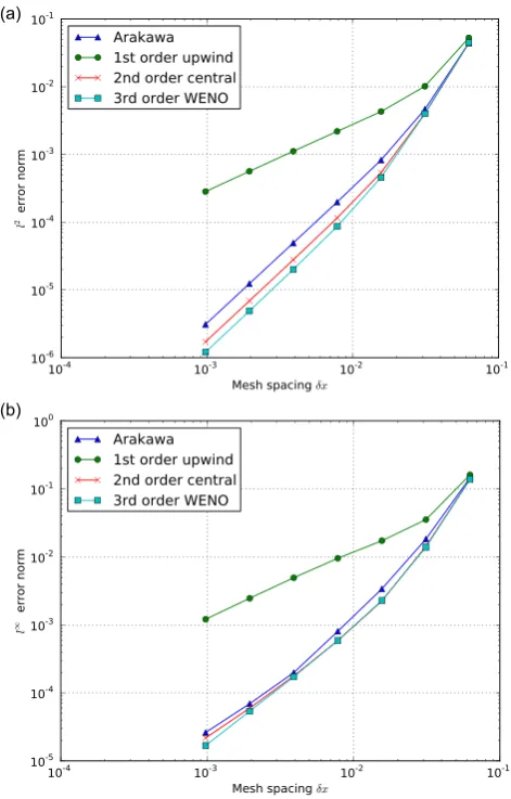
where the coordinates perpendicular to the magnetic field are normalised such that 0x1 and 0z2p. This solu-tion varies smoothly in bothxandz, and in time. Note that the WENO scheme is a limiter scheme, which adapts its stencils depending on the local gradients, and this functional-ity is not properly tested here. Limiter and other adaptive schemes reduce accuracy in steep gradient regions in order to reduce or eliminate overshoot oscillations. This presents a challenge for MMS testing of convergence order, and as far as we are aware there is no accepted means of fully verifying these schemes using the MMS.

Advection schemes require some form of dissipation at the grid scale, in order to avoid numerical oscillations. In the upwind and WENO schemes, this dissipation is provided by upwinding as part of the advection scheme itself, but central differencing schemes such as Arakawa have low dissipation, and require additional dissipation to stabilise the solution, ei-ther physically motivated or numerical. Since ei-there is no other dissipation in this toy problem, a 4th-order hyper-diffu-sion term is added to Equation (12), with a coefficient H

which converges to zero atdx4 _{for grid spacingdx. Without} this dissipation term convergence is typically reduced to first order and becomes dependent on the integration time due to the growth of numerical oscillations. When dissipation with

H¼20 is included, the results are shown in Figure3. Both global error and local error are found to converge at the expected rate in the asymptotic (small dxregime, as measured by the l2

(RMS) error in Figure3(a), and the l1

(maximum) error in Figure 3(b), respectively). Apart from the first order upwind scheme, all schemes converge at sec-ond order in grid spacingdx: The WENO scheme is formally third order accurate in the bulk of the domain, but the advec-tion velocity is calculated from / using 2nd-order central differences, and boundary conditions are only second-order accurate, reducing the overall convergence rate to second order. The WENO scheme implementation cannot therefore be considered fully verified, and as noted above the verifica-tion of limiter schemes using MMS remains an outstanding problem, and so we leave this for further work.

C. Schemes for wave equations

Along the magnetic field methods are implemented which model wave propagation, such as sound and shear

FIG. 2. Error norm for explicit time integration schemes. Measured conver-gence rates based on the two highest resolution cases are: 0.995 (Euler), 2.13 (Karniadakis), 3.00 (RK3-SSP), and 3.99 (RK4). Script:examples/ MMS/time/runtest.

Alfven waves, and diffusion processes such as heat conduc-tivity. Wave propagation operators often appear in the form of coupled first order equations

@f

@t¼

@g

@x

@g

@t ¼

@f

@x: (15)

The manufactured solution was chosen to be

f ¼0:9þ0:9xþ0:2 cosð10tÞsinð5x2Þ;

g¼0:9þ0:7xþ0:2 cosð7tÞsinð2x2Þ;

and the equations are solved using staggered 2nd-order cen-tral differencing: Variablegwas shifted to the cell bounda-ries, whilst f was cell centred. This arrangement requires different handling of boundary conditions to account for this shift. To test boundary conditions and handling of staggered variables, this test was performed inxand then iny (replac-ingxwithy=2pin the above manufactured solutions).

Results of a convergence test are shown in Figure 4,

which shows thel2 (RMS) andl1 _{(maximum) error norms}

for quantity f as a function of the mesh spacing dx. This shows convergence at an order around 1.97, as expected for this scheme. This test has been conducted with combinations of Dirichlet and Neumann boundary conditions, finding essentially the same result in all cases.

D. Second derivative operators

In order to verify the second derivative (diffusive) oper-ators and boundary conditions, a series of tests have been performed: First, we verify the spatial convergence rate towards a steady state (time-independent) manufactured so-lution; and then we verify using a time-dependent manufac-tured solution.

1. Steady-state manufactured solution

In order to verify spatial convergence for time-dependent systems of equations, the approach taken in Ref.5 is to evolve the equations towards a steady-state solution. Here, we use this approach to verify boundary conditions and second-order operators by solving the equation

@f

@t ¼

@2_f

@x2þS: (16)

The manufactured solution is chosen to be

fM¼0:9þ0:9xþ0:2 sinð5x2_Þ;

(17)

in the range 0x1, i.e., boundaries are at x¼0 and

x¼1. The source function is therefore

S¼20x2

sinð5x2_Þ

2 cosð5x2_Þ:

(18)

In contrast to the time-dependent MMS tests presented in this paper, for this steady-state problem, we initialise the simulation att¼0 withf¼0, and not the exact manufactured solution. This is suggested in Ref.5since even though this increases the number of iterations to convergence, using the exact solution can hide coding mistakes. Equation (16)was then integrated in time tot¼10 using an absolute tolerance

FIG. 3. MMS test of advection operators. Equation(12)is solved on a 2D domain with uniform grid spacing. The resolution varies from 1616 to 10241024. Convergence rates for second-order Arakawa (1.998), 1st-order upwind (0.993), 2nd-1st-order central differencing (2.005), and 3rd-1st-order WENO (2.019). All methods are limited to at best second-order in mesh spacingdxdue to the central differencing applied to/and the boundary conditions. Script:examples/MMS/advection/runtest.

of 1015 and a relative tolerance of 107. This is a suffi-ciently long time that f reaches a steady state to within tolerances.

Results are listed in Table I, showing l2and l1 errors and convergence rates. We first perform the test with Dirichlet boundary conditions, then with mixed Dirichlet and Neumann conditions. In all cases, 2nd-order convergence is observed at high resolution.

2. Time-dependent manufactured solution

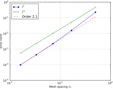
Diffusion equations in all three dimensions, separately and in combination, have been verified, with convergence for one example shown in Figure5. The equation solved is

@f

@t ¼ r

2

f; (19)

which is solved using 2nd-order central differences on a uni-form grid. In 3D the manufactured solution used was

f ¼0:9þ0:9xþ0:2 cosð10tÞsinð5x2

2zÞ þcosðyÞ;

(20)

in the range 0x1; 0y2pand 0z2p. Results

for a uniform 3D grid are shown in Figure5, showing con-vergence at the expected order.

These tests confirm that these simple operators and the Dirichlet and Neumann boundary conditions have been imple-mented correctly for uniform orthogonal grids. More compli-cated geometries are tested in Sec.IV E, but the advantage of these simple tests is that they run in under a minute on a

desk-top and so are now included in the standard BOUTþþ test

suite which is run routinely to check for errors.

E. Coordinate systems

The field-aligned coordinate system used for tokamak simulations has been tested using the analytic input mesh described in SectionIII. The manufactured solution was

f ¼cosð4x4_{þfhÞ þ}

sinðtÞsinð3xþ2fhÞ; (21)

where x¼w=Dw is a normalised radial coordinate with a range between 0 and 1. The safety factor was chosen to be

q¼2þx2

, and inverse aspect ratio¼0:1. Following the procedure outlined in SectionIII, this results in toroidal and poloidal magnetic field components

Bf¼

1

10:1 cosð Þh ; (22a)

Bh¼

0:1

x2_þ2

ð Þ½10:1 cosð Þh2ð1þ0:1 cosð Þh Þ; (22b)

and integrated shear

I¼1125x½hþ0:1 sinðhÞ: (23)

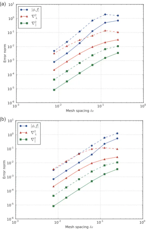
Results are shown in Figure 6for a range of resolutions from 43to 1283, showing convergence of the Arakawa bracket operator ½/;f, a perpendicular diffusion operator r2

?, and

parallel diffusion operatorr2

jj. Tests in both ballooning

coor-dinates (Equation(6), Figure6(a)) and shifted metric (Figure 6(b)) show 2nd order convergence as expected: In addition to verifying these operators in non-orthogonal curvilinear coordi-nates, this test exercises the twist-shift matching used to close field-lines in the core region of tokamak simulations, and the calculation of radial derivatives in the shifted metric scheme. Note that in Figures6(a)and6(b)the parallel diffusion opera-torr2

jjresults are identical, as the use of shifted metrics does

not affect derivatives in the parallel direction (see SectionIII). For this test case, the reference poloidal angle h0 in Equation(10)was set to zero, soI¼0 ath¼0. Ath¼0 the

TABLE I. Error norms and convergence rates for integration of Equation(19)as a function of number of grid pointsN. Shown are cases with Dirichlet bound-ary conditions, then with one Dirichlet and one Neumann boundbound-ary (mixed).

Dirichlet Mixed

N l2

Rate l1 _{Rate l}2

Rate l1 _Rate

8 2.624102 _6.088

102 _3.504

102 _6.317

102

16 4.332103 2.126 1.227102 1.890 5.514103 2.182 1.242102 1.919 32 9.224104 _{2.030 2.720}

103 _{1.978 1.165}

103 _{2.039 2.733}

103 _1.986

64 2.149104 2.007 6.400104 1.993 2.712104 2.009 6.415104 1.997 128 5.199105 _{2.001 1.552}

104 _{1.997 6.554}

105 _{2.003 1.554}

104 _1.999

256 1.271105 2.009 3.822105 1.999 1.607105 2.005 3.825105 2.000 512 3.395106 _{1.894 9.572}

106 _{1.986 4.000}

106 _{1.996 9.488}

106 _2.000

FIG. 5. Error norms for diffusion equation(19)in 3D on a uniform grid as a function of grid spacingdx, showing convergence with an order of 2.06. Script:examples/MMS/diffusion2/runtest.

x–zmesh is therefore orthogonal, and there is no difference between ballooning and shifted metric results in Figure7at this location in h. Moving away fromh¼0 the x–zmesh becomes increasingly deformed, and differences between the ballooning and shifted-metric procedures become apparent. As expected, the error norm is largest close toh¼2pwhere the mesh is most sheared, and the error at this point is reduced significantly by using the shifted metric procedure. The shifted metric method is however not always more accu-rate than the ballooning coordinate method, as shown for the advection operator around h¼p=4 in Figure 7, where the ballooning coordinates are more accurate: In general, the ac-curacy of these methods will depend on the solution. It has been found in simulations of Edge Localised Modes with BOUTþþ30,31

that the use of the shifted metric method improves numerical stability at the twist-shift location where the mesh deformation changes abruptly. This coordinate sys-tem is used in Section V B to verify the 3-field equations used for edge localised modes (ELM) simulations.

F. Flux coordinate independent scheme

To verify the interpolation and central differencing

schemes implemented in BOUTþþfor FCI coordinates, we

simulate a wave (Equation (15)) in a sheared slab. On each

x –zplane perpendicular to the magnetic field a Cartesian mesh is used, and the magnetic field is sheared so that the points to be interpolated (small open circles in Figure 1) span a range of locations between neighbouring grid points.

A sheared slab of size Ly¼10 m along the magnetic

field;Lx¼0:1 m in the radial direction, andLz¼1 m in the

binormal direction was used, with magnetic field

ðBx;By;BzÞ ¼ ð0;1;0:05þ ðx0:05Þ=10Þ. The variation of

the magnetic field-line pitch withxtherefore ensures that the interpolation location varies so as to test the 3rd-order Hermite interpolation scheme. The manufactured solution used was

f ¼sinðyzÞ þcosðtÞsinðy2zÞ; (24a)

g¼cosðyzÞ þcosðtÞsinðy2zÞ; (24b)

whereyandzare normalised to be between 0 and 2pin the domain (as in all manufactured solutions presented here).

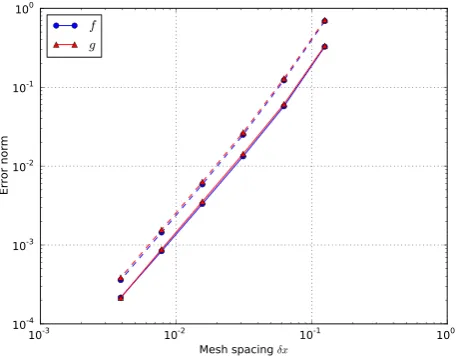
Figure8shows the error norm as the resolution in both parallel and perpendicular directions is varied. This shows second-order convergence, most likely limited by the accu-racy of the second-order central differencing scheme used to calculate parallel derivatives. Note that in order to obtain good convergence, it was necessary to stabilise the collo-cated scheme, by adding a parallel diffusion term of the form

dx2_@2

jj to each equation. This has been previously discussed

in the context of MMS testing of collocated numerical schemes in Ref.5.

V. MODELS

After verification of individual operators, the MMS technique is now applied to the verification of entire models, which combine operators and couple multiple fields. Here, three models of interest are verified: the 2-field

Hasegawa-Wakatani system (Section V A), a 3-field reduced MHD

model which has been used extensively to simulate Edge

Localised Modes (ELMs) with BOUTþ þ (Section V B),

FIG. 6. Verification of operators in toroidal field-aligned coordinates. Coordinate system and input described in SectionIII. Script:examples/ MMS/tokamak/runtest.

and a 5-field cold-ion model for tokamak edge turbulence (SectionV C).

Due to the large number of models which have been

implemented in BOUTþþ, we have introduced a naming

scheme which can be used in future publications to refer to a

specific model. A scheme BOUTþþ/name/year such as

BOUTþþ/HW/2014 is used here.

A. Hasegawa-Wakatani (BOUT11/HW/2014)

The Hasegawa-Wakatani model is a good starting place as it contains many of the elements of more complicated models, such as Poisson brackets, diffusion, and calculation of electrostatic potential from vorticity, whilst being 2D and faster to run than 3D models at high resolutions. As such, it often forms a starting point for the construction of more complex models. The equations solved are for plasma den-sitynand vorticityx¼~b0 r ~vwhere~vis the EB drift velocity in a constant magnetic field, and~b0is the unit vector in the direction of the equilibrium magnetic field

@n

@t ¼ ½/;n þa /ð nÞ j

@/

@zþDnr

2

?n; (25a)

@x

@t ¼ ½/;x þa /ð nÞ þDxr

2

?x; (25b)

r2

?/¼x: (25c)

The manufactured solutions were chosen to be

n¼0:9þ0:9xþ0:2 cosð10tÞsinð5x22zÞ; (26a)

x¼0:9þ0:7xþ0:2 cosð7tÞsinð2x2

3zÞ; (26b)

/¼sinðpxÞ½0:5xcosð7tÞsinð3x23zÞ; (26c)

along with parameters

a¼1 j¼1

2 Dn¼1 Dx¼1: (27)

These parameters were chosen so that the magnitude of each term in Equation(25)was comparable; in a realistic simula-tion the parameters might be different, in particular, the diffu-sion termsDn;xwould generally be smaller than is used here. This does not present a problem for verification, since the cor-rectness of the numerical method implementation does not depend on these parameters. If the code is correct withDn¼1

then it will also be correct with Dn¼105. This does not

guarantee that the method will be stable with arbitrary param-eters, and in general, the required resolutions and stability cri-teria (e.g., maximum timestep) will be problem specific.

Note that the solution for both vorticityxand potential

/are manufactured, despite the two quantities being related through the vorticity equation(25c). This avoids integration of manufactured solutions and is handled by adding an ana-lytic source term to the right hand side of Equation(25c).

Results are shown in Figure9, calculated on a 2D unit domain, showing thel2andl1norms over bothnandx, and a fit showing second order convergence. This shows that the operators in Equation(25)including the inversion of poten-tial/from vorticityxare correctly implemented, at least on orthogonal uniform grids. We now proceed to test these operators in toroidal field-aligned coordinate systems typical of realistic BOUTþþsimulations.

B. 3-field reduced MHD (BOUT11/FLUID3/2014)

The 3-field model used for ELM simulations1,30,31 has been verified in field-aligned toroidal geometry with a radi-ally varying safety factorq, using the shifted metric coordi-nate system described in Section III, and tested in Section IV E. This is in order to verify the methods implemented in

BOUTþþ in coordinate systems with a non-trivial metric

tensor.

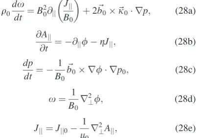
The equations evolved are for vorticityx¼b~0 r ~v, pressurep, and the parallel component of the magnetic vec-tor potentialAjj¼~b0A~, where~b0¼

~ B0

jB~0j;

~

B0is the unit

vec-tor along the equilibrium magnetic fieldB~0, andB0¼ jB~0jis the magnitude of the magnetic field

FIG. 8. Convergence off(1.95) andg(2.04) in Equation(15)solved using the FCI method in a sheared slab. Solid lines showl2

(RMS) error, whilst dashed lines show l1 (maximum) error. Script:examples/fci-slab/ runtest

FIG. 9. Error norm of Hasegawa-Wakatani system (nand/, Equation(25)) on a Cartesian mesh, showing second-order convergence. Mesh resolutions range from 1616 to 512512. Script:examples/MMS/hw/runtest.

q0

dx

dt ¼B

2 0@jj

Jjj B0

þ2b~0~j0 rp; (28a)

@Ajj

@t ¼ @jj/gJjj; (28b)

dp dt ¼

1

B0

~

b0 r/ rp0; (28c)

x¼ 1

B0

r2

?/; (28d)

Jjj¼Jjj0 1

l0

r2

?Ajj; (28e)

where the parallel derivative includes the perturbed magnetic field

@jj¼~b0 r 1

B0

~

b0 rAjj r; (29)

where “0” subscripts denote equilibrium (starting) quanti-ties: q0is the (constant) density; B~0 is the magnetic field; and j0¼ ð~b0 rÞ~bis the field-line curvature. The electro-static potential/is calculated from the vorticity by invert-ing a perpendicular Laplacian (with Dirichlet boundary conditions here), and the parallel currentJjj¼~b0~J is cal-culated from the vector potential. The convective derivative is defined as

d dt¼

@ @tþ

1

B0

~

b0 r/ r: (30)

Background (equilibrium) profiles are chosen to mimic real-istic cases, with a pedestal-like pressure profileP0, and a

par-allel current profile J0 which peaks on the outboard and

inboard midplanes

P0=P¼2þcosðpxÞ J0=J¼1xþsin2ðpxÞcosðhÞ; (31)

where x is the normalised radial coordinate, which lies

between 0 and 1, and h is the poloidal angle, which lies

between 0 and 2p. Normalisation parameters are

ne¼1019m3; Te¼3 eV; L¼1m; B¼1T;

P¼2eneTe¼9:6 Pa; J¼B=ðl0LÞ: (32)

The manufactured solutions used were

/¼ ½sinðzxþtÞ þ103cosðyzÞsinð2pxÞ; (33a)

w¼104cosð4x2þzyÞ; (33b)

U¼2 sinð2tÞcosðxzþ4yÞ; (33c)

P¼1þ1

2cosð Þt cos 3x 2

2z

ð _{Þ þ}5103sinðyzÞsinð Þt :

(33d)

A Lundquist number ofS¼10 was used to set the resis-tivity g. This is so that the resistive term in Ohm’s law

(Equation (28b)) becomes comparable to the other terms,

andSis much smaller (higherg) than would be the case in a realistic tokamak simulation, for which S¼108 would be more typical.

Results are shown in Figure10, with thel2andl1norms shown for each evolving variableðP;w;UÞ. The slow con-vergence at large mesh spacing (small resolution) is due to the solutions being under-resolved: the smallest grids have only 4 grid points in each dimension, insufficient to resolve the manufactured solution. At high resolution, the pressure and electromagnetic potential fields converge at 2nd order as expected, but the vorticityxconverges at a rate between the first and second order. The maximum (l1) error in vorticity converges at close to 1st order at high resolution, indicating that the source of this slow convergence is an order 1 error on a sub-set of the domain, so that when averaged over the domain the RMS (l2

) error converges at a faster rate than the maximum error. The location of the error maximum at high resolution is at the radial boundary, but the reason for this is not yet clear despite extensive investigation. Here, we clude that although the model does converge, it does not con-verge at the expected rate, and further investigation is needed.

C. BOUT11/FLUID5/2014

Finally, the set of equations implemented in the Global

Braginskii Solver (GBS) code32 have been implemented in

BOUTþþ and verified in a simplified form using the

Method of Manufactured Solutions. In this current work, electromagnetic effects and ion viscosity terms were neglected. The equations are for plasma density n, electron temperatureTe, vorticityx, Ohm’s law, and parallel ion

ve-locityVjji

@n

@t ¼ R

qs0 1

B½/;n þ

2n

B C Tð Þ þe T

nC nð Þ Cð Þ/

nð~b rÞVjjeVjjeðb~ rÞnþD nð Þ þS; (34a)

FIG. 10. Error norms for 3-field set of equations. Solid lines show thel2

(RMS) error norms, whilst dashed lines are the l1 _{(maximum) error.}

Convergence orders for pressurepis 1.95; vorticityxis 1.64; and vector potentialAjjis 2.01. Resolutions range from 43to 1283. Sctript:examples/

@Te

@t ¼ R

q_s0 1

B½/;Te Vjjeðb~ rÞTe

þ4

3

Te B

7

2C Tð Þ þe

Te

nC nð Þ Cð Þ/

þ2Te

3

0:71ð~b rÞVjji1:71ðb~ rÞVjje

þ0:71 VjjiVjje

n ð~b rÞn

þDTeð Þ þTe DjjTeð Þ þTe ST; (34b)

@x

@t ¼ R

q_s0 1

B½/;x Vjjiðb~ rÞx

þB2 ð~b rÞVjjiVjjeþ

VjjiVjje

n ð~b rÞn

þ2B C Teð Þ þTe nC nð Þ

þDxð Þx ;

(34c)

@Vjje

@t ¼ R

q_s0 1

B /;Vjje

Vjjeð~b rÞVjje

mi me

VjjeVjjiþ mi me

~

b r ð Þ_/

miTe

nmeð~b rÞn1:71 mi

með~b rÞTeþDVjje Vjje

_;

(34d)

@Vjji

@t ¼ R

qs0 1

B /;Vjji

Vjjið~b rÞVjji

ð~b rÞTeþ Te

nð~b rÞnþDVjji Vjji

_;

(34e)

where

q_s0¼

Cs0 Xci

Cs0 ¼ ffiffiffiffiffiffiffiffi

eTe mi

s

Xci¼ eB

mi

; (35)

with vorticity and the curvature operator defined as

x¼ r2

?/ C Að Þ ¼ B 2 r ~ b B

rA: (36)

Here, the dissipation operators DðÞ were hyper-diffusion terms in the plane perpendicular to the magnetic field of the form

D fð Þ ¼ dx4@ 4_f

@x4dz 4@

4_f

@z4: (37)

In order to test all terms in this set of equations, the pa-rameters of the simulation should be chosen so that the mag-nitude of each term is of a similar order of magmag-nitude. If this is not done, then the error in the result will be dominated by a small number of operators, and mistakes in the implemen-tation of small terms may not become apparent until very high (possibly impractical) resolution is reached. In order to handle the large number of terms in Equations(34a)–(34e), the magnitude of each term was estimated using SymPy by replacing trigonometric functions sinðÞand cosðÞby their

maximum value (1), and the coordinates ðx;h;fÞ by their maximum valuesð1;2p;2pÞ. This allowed parameters to be quickly adjusted to find useful regimes. The resulting manu-factured solutions are

n¼0:9þ0:9xþ0:5 cosðtÞsinð5x2zÞ þ0:01

sinðyzÞ; (38a)

Te¼1þ0:5 cosðtÞcosð3x22zÞ þ0:005 sinðyzÞsinðtÞ;

(38b)

x¼2 sinð2tÞcosðxzþ4yÞ; (38c)

Ve¼cosð1:5tÞ½2 sinððx0:5Þ2þzÞ

þ0:05 cosð3x2þyzÞ; (38d)

Vi¼ 0:01 cosð7tÞcosð3x2þ2y2zÞ; (38e)

/¼ ½sinðzxþtÞ þ0:001 cosðyzÞsinð2pxÞ: (38f)

Parameters used were

Te¼3 eV; ne¼1019m3; B¼0:1T; mi¼0:1mp;

(39)

wherempis the mass of the proton. Light ions were used in

order to reduce the difference in timescales between elec-trons and ion dynamics. Note that the manufactured solutions and parameters are not required to be realistic, provided that they do not violate any constraints such as positivity of den-sity and temperature, as discussed in SectionII.

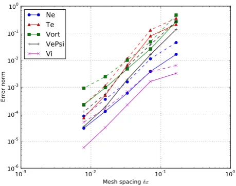
Simulations were performed in a 3D slab geometry, with resulting error norms shown in Figure 11. In this geometry, the curvature polarisation vectorr ~b

B is set to a constant in

thez(binormal) direction. All fields show convergence at the expected rate, approximately 2nd-order in mesh spacing dx. This demonstrates that complex models can be verified using the method of manufactured solutions in BOUTþþ.

FIG. 11. Error norms for 5-field set of equations. Solid lines show thel2

(RMS) error norms, whilst dashed lines are the l1 _{(maximum) error.}

Convergence orders for densityNeis 2.02; electron temperatureTeis 2.70; vorticityxis 2.04; electron parallel velocityVeis 2.36; and ion velocityVi is 2.42. Resolutions range from 83_{to 128}3_{. Script:examples/MMS/GBS/}

runtest-slab3d.

VI. CONCLUSIONS AND DISCUSSION

The Method of Manufactured solutions have been used to rigorously test numerical methods implemented in BOUTþþ, both independently as unit tests, and in combina-tion as simulacombina-tion models. Convergence to the correct solu-tion at an asymptotic 2nd order has been demonstrated for

large sub-sets of the BOUTþþ framework: Though higher

order methods (3rd-order WENO and 4th-order central

dif-ferencing) are implemented in BOUTþþ, the overall

con-vergence rate is limited to 2nd order by the boundary conditions.

Mechanisms have been implemented into BOUTþþ,

which simplify and partly automate the process of verifying the correctness of a numerical implementation, requiring minimal modifications to the code between production simu-lations and verification runs. This will facilitate the routine use of the MMS as an increasing variety of models are

implemented in BOUTþþ. Since code verification is an

ongoing process, particularly for an actively developed

sci-entific code such as BOUTþþ, the methods and tests

detailed here are now used as part of a test suite which is run routinely and automatically (using Travis-CI) to test every

change made to BOUTþþ.

It is important to note the limitations of the present work, which will be the subject of further development. Whilst curvilinear coordinates in tokamak geometry with varying safety factor have been verified, no tests have yet been performed in X-point geometry. The Flux Coordinate Independent (FCI) scheme has been implemented in

BOUTþþ, but only tested in sheared slab geometry.

Investigation of methods for simulations of X-point geome-try, including FCI, and verification with MMS will be the subject of future work.

ACKNOWLEDGMENTS

This work has been carried out within the framework of the EUROfusion Consortium and has received funding from the Euratom research and training programme 2014-2018 under Grant Agreement No. 633053. The views and opinions expressed herein do not necessarily reflect those of the European Commission. The authors gratefully acknowledge the support of the UK Engineering and Physical Sciences Research Council (EPSRC) under Grant No. EP/K006940/1, and Archer computing resources under Plasma HEC consortium Grant No. EP/L000237/1.

1_{B. D. Dudson, M. V. Umansky, X. Q. Xu, P. B. Snyder, and H. R. Wilson,}

Comput. Phys. Commun.180, 1467–1480 (2009).

2_{B. D. Dudson, A. Allen, G. Breyiannis, E. Brugger, J. Buchanan, L. Easy,}

S. Farley, I. Joseph, M. Kim, A. D. McGannn, J. T. Omotani, and M. V. Umansky,J. Plasma Phys.81_{(01), 365810104 (2015).}

3

P. J. Roache,Verification and Validation in Computational Science and Engineering(Hermosa Publishers, Albuquerque, NM, 1998).

4

W. L. Oberkampf and C. J. Roy,Verification and Validation in Scientific Computing(Cambridge University Press, New York, NY, USA, 2010).

5_{K. Salari and P. Knupp, “Code verification by the method of manufactured}

solutions,” Technical Report No. SAND2000-1444, Sandia National Laboratories, 2000.

6_{M. V. Umansky, R. H. Cohen, L. L. LoDestro, and X. Q. Xu,Contrib.}

Plasma Phys.48(1–3), 27–31 (2008).

7

C. J. Roy, C. C. Nelson, T. M. Smith, and C. C. Ober, Int. J. Num. Methods Fluids44_{(6), 599–620 (2004).}

8_{D. Kalupin, V. Basiuk, D. Coster, Ph. Huynh, L. L. Alves, Th. Aniel, J. F.}

Artaud, J. P. S. Bizarro, C. Boulbe, R. Coelho, D. Farina, B. Faugeras, J. Ferreira, A. Figueiredo, L. Figini, K. Gal, L. Garzotti, F. Imbeaux, I. Ivanova-Stanik, T. Jonsson, C. J. Konz, E. Nardon, S. Nowak, G. Pereverzev, O. Sauter, B. Scott, M. Schneider, R. Stankiewicz, P. Strand, I. Voitsekhovitch, ITM-TF Contributors, and JET-EFDA Contributors, in Europhysics Conference Abstracts Proceedings of the 35th EPS Conference on Plasma Physics, Hersonissos, Crete(2008), Vol. 32D, p. P–5.027.

9_{C. S. Chang, S. Ku, P. Diamond, M. Adams, R. Barreto, Y. Chen, J.}

Cummings, E. D’Azevedo, G. Dif-Pradalier, S. Ethier, L. Greengard, T. S. Hahm, F. Hinton, D. Keyes, S. Klasky, Z. Lin, J. Lofstead, G. Park, S. Parker, N. Podhorszki, K. Schwan, A. Shoshani, D. Silver, M. Wolf, P. Worley, H. Weitzner, E. Yoon, and D. Zorin, J. Phys.: Conf. Ser.180, 012057 (2009).

10

F. Riva, P. Ricci, F. D. Halpern, S. Jolliet, J. Loizu, and A. Mosetto,Phys. Plasmas21, 062301 (2014).

11_{C. Michoski, D. Meyerson, T. Isaac, and F. Waelbroeck, “Discontinuous}

galerkin methods for plasma physics in the scrape-off layer of tokamaks,” J. Comput. Phys.274_{, 898–919 (2014).}

12_{SymPy Development Team (2016), SymPy: Python library for symbolic}

mathematics,http://www.sympy.org(seehttps://github.com/sympy/sympy).

13

R. LeVeque, Finite Difference Methods for Ordinary and Partial Differential Equations(SIAM, 2007).

14_{W. D. Haeseler, Flux Coordinates and Magnetic Field Structure}

(Springer, 1991).

15

X. Q. Xu, M. V. Umansky, B. Dudson, and P. B. Snyder, “Boundary plasma turbulence simulations for tokamaks,”Commun. Comput. Phys. 4(5), 949–979 (2008).

16_{A. M. Dimits,Phys. Rev. E48(5), 4070–4079 (1993).} 17

B. Scott,Phys. Plasmas8_{(2), 447 (2001).} 18

F. Hariri and M. Ottaviani,Comput. Phys. Commun.184_{(11), 2419–2429} (2013).

19_{A. Stegmeir, D. Coster, O. Maj, and K. Lackner,Contrib. Plasma Phys.} 54_{, 549–554 (2014).}

20

A. Iserles, A First Course in the Numerical Analysis of Differential Equations(Cambridge University Press, 2009), ISBN: 978-0-521-73490-5.

21

G. E. Karniadakis, M. Israeli, and S. A. Orszag,J. Comput. Phys.97_{, 414} (1991).

22_{B. D. Scott, “Free-energy conservation in local gyrofluid models,”Phys.}

Plasmas12, 102307 (2005).

23

S. Gottlieb, C.-W. Shu, and E. Tadmor,SIAM Rev.43_{(1), 89–112 (2001).} 24

A. C. Hindmarsh, P. N. Brown, K. E. Grant, S. L. Lee, R. Serban, D. E. Shumaker, and C. S. Woodward, “SUNDIALS: Suite of nonlinear and dif-ferential/algebraic equation solvers,”ACM Trans. Math. Software31(3), 363–396 (2005).

25

S. Balay, W. D. Gropp, L. C. McInnes, and B. F. Smith, in Modern Software Tools in Scientific Computing, edited by E. Arge, A. M. Bruaset, and H. P. Langtangen (Birkhauser Press, 1997), pp. 163–202.

26

S. Balay, S. Abhyankar, M. Adams, J. Brown, P. Brune, K. Buschelman, V. Eijkhout, W. Gropp, D. Kaushik, M. Knepley, L. C. McInnes, K. Rupp, B. Smith, and H. Zhang, Technical Report No. ANL-95/11—Revision 3.5, Argonne National Laboratory, 2015.

27

A. Arakawa,J. Comput. Phys.1_{, 119–143 (1966).} 28

G.-S. Jiang and C.-W. Shu,J. Comput. Phys.126_{, 202–228 (1996).} 29_{G.-S. Jiang and D. Peng,SIAM J. Sci. Comput.21(6), 2126–2143 (2000).} 30_{X. Q. Xu, B. Dudson, P. B. Snyder, M. V. Umansky, and H. Wilson,Phys.}

Rev. Lett.105_{, 175005 (2010).} 31

B. D. Dudson, X. Q. Xu, M. V. Umansky, H. R. Wilson, and P. B. Snyder, Plasma Phys. Controlled Fusion53, 054005 (2011).

32_{P. Ricci, F. D. Halpern, S. Jolliet, J. Loizu, A. Mosetto, A. Fasoli, I. Furno,}