Extrapolating demography with climate, proximity and phylogeny: approach with caution

White Rose Research Online URL for this paper: http://eprints.whiterose.ac.uk/106767/

Version: Accepted Version

Article:

Coutts, S.R., Salguero-Gomez, R., Csergo, A.M. et al. (1 more author) (2016)

Extrapolating demography with climate, proximity and phylogeny: approach with caution. Ecology Letters, 19 (12). pp. 1429-1438. ISSN 1461-0248

https://doi.org/10.1111/ele.12691

Reuse

Unless indicated otherwise, fulltext items are protected by copyright with all rights reserved. The copyright exception in section 29 of the Copyright, Designs and Patents Act 1988 allows the making of a single copy solely for the purpose of non-commercial research or private study within the limits of fair dealing. The publisher or other rights-holder may allow further reproduction and re-use of this version - refer to the White Rose Research Online record for this item. Where records identify the publisher as the copyright holder, users can verify any specific terms of use on the publisher’s website.

Takedown

If you consider content in White Rose Research Online to be in breach of UK law, please notify us by

proximity and phylogeny: approach with

caution

Shaun R. Coutts

, Roberto Salguero-Gómez

, Anna M. Csergő

,

Yvonne M. Buckley

October 31, 2016

1. School of Biological Sciences. Centre for Biodiversity and Conservation Science. The University of

Queensland, St Lucia, QLD 4072, Australia.

2. Department of Animal and Plant Sciences, University of Sheffield, Western Bank, Sheffield, UK.

3. School of Natural Sciences, Zoology, Trinity College Dublin, Dublin 2, Ireland.

4. Evolutionary Demography Laboratory. Max Planck Institute for Demographic Research. Rostock,

DE-18057, Germany.

Keywords: COMPADRE Plant Matrix Database, comparative demography, damping ratio, elasticity, matrix population model, phylogenetic analysis, population growth rate (λ), spatially lagged models

Author statement: SRC developed the initial concept, performed the statistical analysis and wrote the

first draft of the manuscript. RSG helped develop the initial concept, provided code for deriving

de-mographic metrics and phylogenetic analysis, and provided the matrix selection criteria. YMB helped

develop the initial concept and advised on analysis. All authors made substantial contributions to editing

ABSTRACT

INTRODUCTION

Global threats to biodiversity such as climate change, invasive species and land conversion for agriculture affect multiple species at regional and global scales (McGeoch et al., 2010; Hartmann et al., 2013). Invasion and extinc-tion are fundamentally demographic processes, regulated by the vital rates of the population (e.g. survival, growth, reproduction). Consequently, we are pressed to understand and predict how demography responds to environmen-tal conditions across multiple taxa worldwide (Sutherland et al., 2013). His-torically, developing such a predictive framework has proven difficult. Even describing demographic patterns across species and regions is challenging due to the lack of both detailed demographic data for multiple species at large geographic scales, and high resolution comparative approaches (but see Blomberg & Garland 2002, Buckleyet al.2010, Salguero-Gómezet al.2016). Another challenge is that we often do not understand the underlying factors that drive population responses to environmental gradients (Ehrlén & Mor-ris, 2015). Further, determining the response of every population of every species is impractical. Consequently, we frequently generalize important as-pects of population ecology, such as life history strategy (Silvertown et al., 1996; Salguero-Gómez et al., 2016) and invasiveness (Ramula et al., 2008), from a handful of well studied species and populations to wider areas and other species.

Even though demographic studies have been carried out on thousands of species, most of those species have only been studied in a few locations. It is common to then assume that those studies adequately capture the demo-graphic performance of a species across an entire region (Burns et al., 2010; Croneet al., 2011; Salguero-Gómezet al., 2016). However, it is currently un-known how close, both geographically and phylogenetically, populations or species must be before demographic performance can be extrapolated among them. Likewise, it remains unknown which aspects of demographic perfor-mance (e.g. population growth rate, recovery from perturbations) are most transferable across populations.

(Salguero-Gómezet al., 2015). Matrix population models are typically constructed from field measurements and summarise life histories ranging from simple to com-plex in a standard format (Caswell, 2001). This allows the direct comparison of ecologically and biologically meaningful demographic metrics across pop-ulations, species and years (Silvertown et al., 1993; Caswell, 2001; Salguero-Gómez & de Kroon, 2010). These metrics include population growth rate (Tuljapurkar & Orzack, 1980; Caswell, 2001), the underlying impacts of de-mographic processes (i.e. vital rates of survival, growth and reproduction) on population performance (de Kroonet al., 1986; Caswell, 2001), or the ability of populations to recover from perturbations (Stott et al., 2010).

We focused on the generalisability of four demographic metrics across species and populations: the asymptotic population growth rate (λ), its variation over time, elasticities of λ to demographic proccesses, and damping ratio (ρ). Previous comparative studies have found that populations of the same species tend to have similar values forλ(Doak & Morris, 2010; Villellaset al., 2015), although other work has shown significant differences among popula-tions of the same species (Silvertownet al., 1996). Comparative studies have found that phylogenetic relationships above the species level do not predict

λ (Buckley et al., 2010; Burns et al., 2010). Environment has been found to explain some variation inλ (Buckleyet al., 2010). However, the effect of any one environmental variable on λ may be reduced as multiple environmental factors can affectλ. In addition, stable populations can be maintained across environmental gradients by increasing some vital rates to offset decreases in others (Doak & Morris, 2010; Villellas et al., 2015). Temporal variation of population growth rates is expected to increase with increasing environmen-tal constraints due to limitations on vienvironmen-tal rates (Gerst et al., 2011). Less evidence exists on how geographic proximity and phylogeny predict elastici-ties and damping ratio. However, plant growth form affects which vital rates are most important for population growth (Enright et al., 1995; Franco & Silvertown, 2004; Salguero-Gómez et al., 2016). Further, we expect that in general species which are closely related are more likely to have the same growth form, although there are exceptions (Mack, 2003; Salguero-Gómez

corre-lated (Fox et al., 2008; Premoli & Kitzberger, 2005), we expect the damping ratio to be predicted by geographically near populations.

Here we examine how transferable these four demographic metrics are across space and phylogeny. We also estimate how far, on average, these demo-graphic measures can be extrapolated. Using the largest dataset of geo-located demographic models currently available, we show that while demo-graphic metrics are predictable to some extent using neighbouring popula-tions and related species, caution must be used in extrapolating demographic data.

MATERIALS AND METHODS

We tested the cross-population, cross-species generalisability of four different aspects of population performance using matrix population models (matrix models, hereafter) from the COMPADRE Plant Matrix Database (COM-PADRE henceforth; Salguero-Gómez et al. 2015). This version of COM-PADRE (obtained 24th October 2014) is included in Appendix 1, Supporting Information. The current version of COMPADRE Plant Matrix database is available at http://www.compadre-db.org/Data/Compadre.

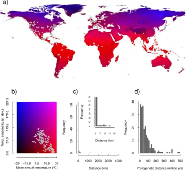
tions. Further details on matrix model selection are described in Appendix 2. These criteria resulted in 550 matrix models for our analysis, covering 210 plant species from 156 genera and 66 families (Table S1, Appendix 2), with populations from tropical regions to the high latitudes (Figure 1a).

a)

Mean annual temperature (°C)

T

emp

. seasonality (st. de

v.)

b)

−29 −13.8 1.5 16.8 32

0.6

57.3

113.9

170.6

227.2

Distance (km)

Frequency

0 1000 2000 3000 4000

0

20

40

60

80

c)

Distance (km)

Frequency

0 5 10 15 20

0

10

20

30

40

50

60

70

Phylogenetic distance (million yrs)

Frequency

0 100 200 300 400 500

0

10

20

30

40

d)

Figure 1. Locations of the 550 populations used in the analysis plotted on, a) world

map coloured with mean annual temperature (◦_{C) and temperature seasonality (standard}

The demographic data are confounded in three different ways. First, some matrix models were built with data from almost the same geographic lo-cation and those populations are likely to experience similar environmental conditions (Figure 1c). Secondly, some species have closer phylogenetic re-lationships to others, thus, any demographic signatures that may be due to phylogenetic constraints must be separated from those that are due to envi-ronmental filtering (Blomberg & Garland, 2002). Further, populations of the same species tended to be at similar geographic locations. Of the 112 species in our dataset that were represented by more than one population, over half (70) had a maximum distance between populations ≤ 2 km, and all but five had a maximum distance between populations≤100 km (Figure 1c). Finally, most (92% of species) of the matrix models for a given species come from a single study. Thus, geographic location, phylogeny and methodological differences between studies are all confounded to some extent, necessitating careful modelling of the data and cautious interpretation of results.

Metrics of demographic performance

We test the transferability of four fundamental metrics of short- and long-term population performance: asymptotic population growth rate, λ, its coefficient of variation through time, CV(λ), the damping ratio, ρ, and a composite axis of matrix element elasticities, the Stasis-Progression Gradient (hereafter SPG).

The damping ratio, ρ, is an index of the rate that a population converges to its stable age or stage distribution after it has been perturbed (Stott et al., 2011), and it has important implications for conservation (Koonset al., 2005; Stott et al., 2011). Values of λ and ρ for each matrix model were calculated with the ’popbio’ R package (Stubben & Milligan, 2007).

Matrix element elasticities of λ are the proportional changes in λ caused by small proportional changes in corresponding matrix elements (Caswell, 2001). Elasticities indicate the relative importance of the demographic transitions of stasis, progression and retrogression, as well as the per capita contributions from sexual reproduction, toλ (de Kroonet al., 1986). After the population growth rate, elasticities are the most commonly used demographic metric in plant population studies (Franco & Silvertown, 2004; Ramula et al., 2008). This is especially true in conservation and invasion biology where stages and demographic processes with the highest elasticities are typically targeted for conservation across wider areas and similar species (Silvertown et al., 1996; Shea & Kelly, 1998; Ramula et al., 2008).

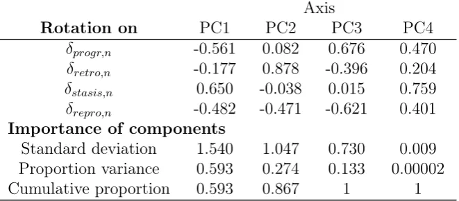
In order to compare matrix element elasticities of λ across populations and species, we classified each matrix element as belonging to the process of reproduction (both asexual and sexual), progression, stasis or retrogression (Silvertownet al., 1993), producing a vector of four elasticities. Because these four elasticities must add up to one (de Kroonet al., 1986), a higher value for one necessitates a lower value for the others. To overcome this limitation, we used Principal Components Analysis (PCA) to reduce the four elasticities to a single axis, PC1, which accounted for 59% of the variance. We term this axis the Stasis-Progression Gradient, SPG. At high SPG scores elasticities of λ to stasis transitions are large (loading 0.65), and elasticities of λ to reproduction and progression transitions are small (loadings -0.48 and -0.56 respectively). The opposite applies to populations with low SPG scores (see Appendix 3, Table S1 for loadings and variance explained by each axis).

Values of λn,ρnand SPGn are derived fromMn, thenth mean matrix model

in our dataset, where each element is the arithmetic mean of the transition rate over the study period. CV(λ)n was calculated from several individual

Predictors of demographic performance

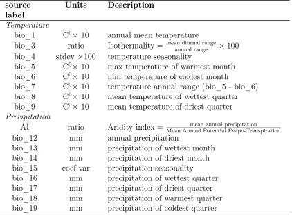
We explained variation in these four demographic metrics of population per-formance using climate, demographic perper-formance at neighbouring locations, and performance in related species, along with matrix model and species level attributes. The location of each matrix model is given by GPS coor-dinates recorded in COMPADRE, which are sourced from publications or through personal communication with the authors (R. Salguero-Gómez, un-publ. data). GPS locations were used to calculate the distance between data collection sites and to extract 16 climatic variables from the BioClim database (bio_1, bio_3 - bio_9, bio_12 - bio_19; www.worldclim.org/bioclim) along with an Aridity index from CGIAR-CSI (http://www.csi.cgiar.org). These variables cover different aspects of the mean and seasonal variability of tem-perature and precipitation, for more details see Table S3, Appendix 4. Cli-mate predictors were extracted from raster files with 30 arc-second resolution. For each location we averaged each climatic variable over a 2km buffer zone to reduce the effect of uncertainty in study location.

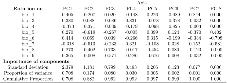
Because the eight temperature variables (Table S3, Appendix 4) were highly correlated with each other we created one composite temperature variable using a Principal Component Analysis (PCA) with the prcomp function of the ’stats’ R library (R Core Team, 2013). The first PC axis, which we refer to as PC_temp, explains 71% of the variance in temperature variables and represents a gradient from cooler seasonably variable temperate climates to hot, non-seasonal tropical climates (see Appendix 3 for more details). The Aridity Index (AI) is positively correlated with all the other precipitation variables in BioClim (Appendix 4, Table S4), except for precipitation sea-sonality (bio_15; Figure S1d, Appendix 3). Thus, we selected Aridity Index and bio_15 to describe precipitation at each location. We log-transformed AI because we expect small absolute differences in water availability have larger effects on population vital rates when water is a limiting factor (i.e. arid areas) (Levine et al., 2008).

We measured phylogenetic relatedness,ti,n, as millions of years since the last

common ancestor of species described by matrix modelsMiandMn. We used

the phylogeny supplied with COMPADRE (Appendix S5; Salguero-Gómez

geographic distance, di,n, as the shortest great arc distance between the

loca-tions of matrix modelsMi and Mn, using the ’Ellipsoidal.Distance’ function

in the ’GEOmap’ R package (Lees, 2015).

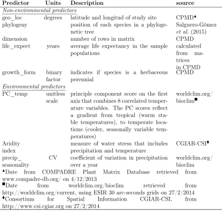
To test if life history traits or matrix model attributes were correlated with demographic performance we used matrix dimension, species’ growth form and mean life expectancy as predictors. Growth form and mean life ex-pectancy have life history trade-off implications that may be reflected in the demographic metrics we test (Silvertown et al., 1993; Enright et al., 1995; Salguero-Gómez & Plotkin, 2010; Stott et al., 2011). Matrix dimension has also been shown to affect the calculation of demographic metrics like ρ and elasticities (Enrightet al., 1995; Salguero-Gómez & Plotkin, 2010; Stottet al., 2010). The ’GrowthType’ variable retrieved from COMPADRE was used to classify species as either herbaceous or non-herbaceous (trees, palms, shrubs, succulents), as non-herbaceous growth forms apart from trees did not have a large enough sample size to fit them individually. At the population level, the fundamental matrix method was used to derive mean life expectancy conditional on having germinated, from each mean matrix (Caswell, 2001, pp. 120). We used the matrix dimension extracted from COMPADRE. See Table S5, Appendix 4 for the list of predictors.

Species

Predictors defined at the species level

●_{Phylogeny is defined at the species level, and thus}

the phylogenetic predictor term, , is defined at the

species level.

●_{Growth type}

Matrix model

Each species is represented by one or more matrix models

Predictors defined at the matrix model level

●Geographic location is defined for each matrix model, and thus the geographic predictor term,

, is defined at the matrix model level.

●Mean life expectancy ●Matrix dimension ●Aridity index ●Precip. seasonality ●Temperature Responses defined

at the matrix model level

●_{Pop. growth rate,} ●_{Coefficient of variation in}

across time, CV() ●_{Damping ratio,} ●_{Stasis progression}

gradient, SPG

Transitions

Each matrix model is based on transition rates from at least 3 years (two observed transitions)

The response variable CV() is based on population

growth rates calculated from each annual transition matrix

Box 1.We use statistical models to explain variation in four demographic metrics (response variables) using environmental and species level predictors, along with neighboring populations and related species. Response and predictor variables in our statistical models are defined at three hierarchical levels:

Statistical analyses

We predicted transformed demographic metrics (ln(λn), ln(CV(λ)n + 1),

ln(ρn), SPGn) using a spatially and phylogenetically lagged, linear model

We define our model as

Yn∼N(µn, σa) (1a)

µn=β0+βX_n+θ_pΦ_n+θ_gΨ_n (1b)

whereYnis the predicted value for one of the transformed demographic

met-rics for matrix model n, drawn from a normal distribution with a standard deviation of σa ∼Gamma(0.0001,0.0001) and a mean of µn. The parameter β0 is the intercept andβis a column vector of slopes. Each slope corresponds

to an effect size of one of the aforementioned predictors or their interactions.

β=



   

β1 β2

...

βK



   

with K being the total number of climatic and species-level predictors in the model. There are six main effect predictors (matrix dimension, growth type, mean life expectancy, PC_temp, Aridity Index, precipitation seasonality), including two-way interactions between the main effects resulted in K = 18. Each slope in β, and the intercept β0, were drawn from wide prior

distribu-tions, βk ∼N(0,0.0001), where N() is a normal distribution. X is a K ×J

matrix of K species-level and climatic predictors, and their interactions, for all J matrix models.

To capture the effect of phylogeny and geographic location, we included a phylogenetic predictor term θpΦn, and a geographic predictor term θgΨn,

respectively (Eq. 2). The terms θpΦn and θgΨn predict the value of Yn as a

weighted average of matrix model n’s relatives or neighbours respectively.

Φn = X

∀i6=n

Yiexp[−φti,n]

X

∀i6=_n

exp[−φti,n]

(2a)

Ψn = X

∀i6=_n

Yiexp[−ψdi,n]

X

∀i6=_n

exp[−ψdi,n]

(2b)

predicting Yn. Similarly ψ ∼Unif(0,1) controls how geographically near vs.

distant neighbours contribute to predictingYn. Whenφorψ are 0, all

popu-lations contribute equally to the prediction ofYnregardless of distance, either

phylogenetic or geographic; asφorψincrease, more closely related species, or geographically closer locations, have a greater contribution to the prediction of Yn. The term ti,n is the phylogenetic distance between species represented

by matrix models i and n. di,n is the geographic distance between the

lo-cations of matrix models i and n. θp ∼ N(0,0.0001) and θg ∼ N(0,0.0001)

are coefficients that scale the phylogenetic and geographic predictions. Any explanatory power from the geographic and phylogenetic predictor terms is a result of spatial auto-correlation in both measured and unmeasured envi-ronmental variables and phylogenetically conserved functional traits, rather than distance per se. If demographic attributes are random with respect to spatially auto-correlated environmental factors, or are not phylogenetically constrained, the phylogenetic and geographic and predictor terms (Φ, and

Ψ respectively) will explain none of the variance in the four demographic metrics tested.

Study, species and location are all to some extent confounded, due to many populations of the same species being from the same study and similar ge-ographic locations. To test the effect this had on the performance of our models, we also tested models where the spatial and phylogenetic predic-tor terms were based on a reduced, but less confounded set of neighbours and relatives. We ran models where Yi in the geographic and phylogenetic

prediction terms (Eq. 2) were only based on matrix models from different locations (that is, where di,n6= 0) or which were based on a different species

(i.e. where ti,n6= 0). We call these ’no_self’ models. In addition, we tested

Table 1. Statistical models used to predict the four demographic metrics, popula-tion growth rate, its temporal varaipopula-tion, damping ratio and the composite elasticites, Statis Progression Gradient (SPG). Because the environmental and species level predic-tors (matrix dimension, growth type, mean life expectancy, first principal component of the temperature variables (PC_temp), Aridity Index, precipitation seasonality) are spa-tially autocorrelated the ’main_int’ and ’main’ models were only fit using geographic and phylogenetic predictor terms based on all 550 matrix models in our dataset.

model name environmental and

species level

pre-dictors

phylogenetic predictor

geographic predictor

main_int All six main effects

and 2-way

inter-actions, giving 18

terms

Based on all populations

main Only the six main

ef-fects

Based on all populations

phygeo-all_pops Not included Based on all populations

phygeo-no_self Not included Based only on

popula-tions that were not of the same species

Based only on popula-tions that were not in the same location

phy-all_pops Not included Based on all

popula-tions

Not included

phy-no_self Not included Based only on

popula-tions that were not of the same species

Not included

geo-all_pops Not included Not included Based on all

popula-tions

geo-no_self Not included Not included Based only on

popula-tions that were not in the same location

geo-graphic location. This raises the general point that these are phenomenolog-ical models which find patterns in the data, patterns which are likely to be caused by multiple related processes acting simultaneously.

RESULTS

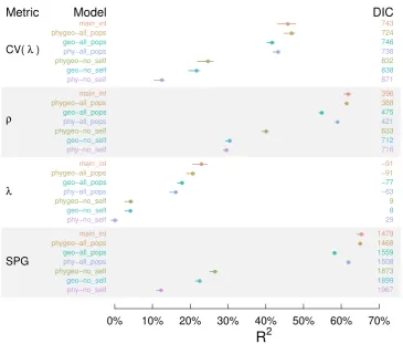
None of the environmental, species- or matrix model level variables had a significant effect on the demographic metrics tested (λ, CV(λ),ρ, and SPG) over and above the effect of the geographic and phylogenetic predictor terms. All of the credible intervals on the coefficients in β, Eq. 1 encompass 0. This is further illustrated by Figure 2, where the full model containing all the predictors did not explain much more variance in any of the demographic metrics than the model that only contained the prediction terms based on geographic and phylogenetic distance (phygeo-allpops). For this reason we do not report results for the ’main’ model as it produced the same results as the ’main_int’ and ’phygeo-all_pops’ models. The ’phygeo’ also had the lowest (or equal lowest) DIC values (Figure 2), suggesting that having both geographic and phylogenetic predictor terms was a good trade-off between parsimony and explanatory power. Overall, models including only predictor terms based on phylogenetic or geographic distance had R2

R

0% 10% 20% 30% 40% 50% 60% 70%

Metric Model DIC

SPG

main_int 1479

phygeo−all_pops 1468

geo−all_pops 1559

phy−all_pops 1508

phygeo−no_self 1873

geo−no_self 1899

phy−no_self 1967

λ

main_int −91

phygeo−all_pops −91

geo−all_pops −77

phy−all_pops −63

phygeo−no_self 9

geo−no_self 8

phy−no_self 29

ρ

main_int 396

phygeo−all_pops 388

geo−all_pops 475

phy−all_pops 421

phygeo−no_self 633

geo−no_self 712

phy−no_self 716

CV( λ )

main_int 743

phygeo−all_pops 724

geo−all_pops 746

phy−all_pops 738

phygeo−no_self 832

geo−no_self 838

phy−no_self 871

Figure 2. We use geographically and phylogenetically lagged statistical models to

explain the variance in four key demographic metrics. We useR2_{to quantify explanatory}

power, higher values indicate more variance explained. MedianR2_{(points) and 95% (solid}

lines) quantiles were taken across 1,500 MCMC samples. Deviance Information Criteria (DIC) is an index of model performance penalized by the number of parameters. Lower DIC numbers indicate more parsimonious models that performed well relative to the other models tested. Note that DIC cannot be compared between metrics, or between ’all_pops’ and ’no_self’ models for the same metric. Colour indicates the model structure. See Table 1 for definitions of ’main_int’, ’phygeo’, ’geo’ and ’phy’ models, and the difference between models with spatial and phylogenetic prediction terms based ’all_pops’ and ’no_self’ predictions.

The best models had R2

pre-dictions were removed several of the ’no_self’ models still explained 20-40% of variation in the metrics of demographic performance (Figure 2).

Our models explained more variation in some metrics of population per-formance than others; with relatively high explanatory power for a matrix model’s position on the SPG continuum and damping ratio (ρ), and lower explanatory power for asymptotic population growth rate (λ) and its tem-poral variation. The best models explained around 65% of the variation in SPG and damping ratio (’main_int’, ’main’ and ’phygeo-all_pops’ density distributions 2) and only 25-45% of variation in CV(λ) and λ. The ’no_self’ models explained between 12-25% of the variation in SPG, 40% of the vari-ation in damping ratio, 5% of the varivari-ation populvari-ation growth rate (λ), and 15-25% of variation in CV(λ) (Figure 2).

For all demographic metrics, exceptρ, the spatial term explained more vari-ation than the phylogenetic term (Figure 2). The ’no_self’ models with only a spatial term explain almost as much variation as models with both a ge-ographic and phylogenetic prediction term (phygeo-no_self in Figure 2). In contrast ’no_self’ models with only a phylogenetic term typically had an R2

about half that of the model including both spatial and phylogenetic terms. Thus, both the spatial and phylogenetic terms are explaining much of the same variance in the response, with the spatial term explaining some variance not explained by phylogenetic term.

To examine the way predictive support drops off with geographic and phy-logenetic distance, we plotted the negative exponential decay models that underpin the geographic and phylogenetic prediction terms (Eq. 2). Here we present decay curves for the ’phygeo-no_self’ model (Table 1), since this model had the lowest DIC of the ’no_self’ models. Results were similar across different models, although uncertainty around the decay curves varies greatly between models (Appendix 5). For models predicting population growth rates (λ) and SPG virtually all predictive support came from loca-tions that were within 15 km of the target location (Figure 3a,c). Predictive support for CV(λ) and damping ratio (ρ) came from locations within 35 km (Figure 3b,d). Predictive support based on phylogeny came from species that diverged <100 mya for SPG, < 20 mya for CV(λ) and < 10 mya for λ and

0 20 40 60 80 100 0.0 0.2 0.4 0.6 0.8 1.0

Geographic dist. (km)

W

eight

a)

0 20 40 60 80 100

0.0 0.2 0.4 0.6 0.8 1.0

Geographic dist. (km)

W

eight

b)

0 20 40 60 80 100

0.0 0.2 0.4 0.6 0.8 1.0

Geographic dist. (km)

W

eight

c)

0 20 40 60 80 100

0.0 0.2 0.4 0.6 0.8 1.0

Geographic dist. (km)

W

eight

d)

0 50 100 150

0.0 0.2 0.4 0.6 0.8 1.0

Phylogenetic dist. (million yrs)

W

eight

e)

0 50 100 150

0.0 0.2 0.4 0.6 0.8 1.0

Phylogenetic dist. (million yrs)

W

eight

f)

0 50 100 150

0.0 0.2 0.4 0.6 0.8 1.0

Phylogenetic dist. (million yrs)

W

eight

g)

0 50 100 150

0.0 0.2 0.4 0.6 0.8 1.0

Phylogenetic dist. (million yrs)

W

eight

h)

Figure 3. Decay curves are the basis of the geographic and phylogenetic predictor terms,

and show how quickly predictive support from neighbouring locations or other species declines with distance (either geographic or phylogenetic). Decay curves for geographic (a-d) and phylogenetic (e-h) predictive terms for each metric, population growth rate (λ), its temporal variation (CV(λ)), Stasis Progression Gradient (SPG) and damping ratio (ρ). The model presented here, phygeo-no_self, has no fixed effects, and predictions were based on geographic locations and species that were different to that being predicted for. Lines show the curve produced by the estimated decay parameter for each of the 1,500 MCMC samples. Grey lines depict the average curve. Average decay curves for other models are generally similar, although the uncertainty around decay curve can vary greatly between different models for the same measure. Decay plots for all other models can be found in Appendix 5.

DISCUSSION

It is common practice in demography, applied ecology and conservation to measure the demography of a species in a few locations and then apply that understanding to the species over a much wider region (Shea & Kelly, 1998; Doak et al., 2005; Crone et al., 2011; Sæther et al., 2005; Salguero-Gómez

et al., 2016). In contrast, we often expect considerable geographic variation in demographic performance of populations within species (e.g., Jongejans & de Kroon 2005, Merow et al. 2014). In our dataset, species and geographic location are too confounded to directly test how transferable demographic information is within species because most populations of the same species were geographically close to each other. However, in our analysis using a dataset of unprecedented size in comparative plant demography, closely re-lated species were much weaker predictors of population performance than geographically close populations. The explanatory power of the geographic predictor term suggests that something about the mid to small-scale envi-ronment is predictive of demography, specifically elasticities of population growth rate, damping ratio and temporal variation in population growth rate. Mid- to small-scale environmental variables will likely include many lo-cal drivers beyond climate, such as soil, anthropogenic impacts (Cole et al., 2014), disturbances and biotic interactions (Silvertown et al., 1996; Thuiller

et al., 2014). It is this mid to small-scale signal that is often lost with global comparisons (Salguero-Gómez et al., 2016).

Borrowing information across closely related species may be more useful for some aspects of demography than others (Blomberg & Garland, 2002). The phylogenetic term unambiguously explained around 10% of the variance in damping ratio over and above the variance explained by the geographic predictor term, much more than the other three demographic metrics. In the case of the damping ratio, only species that diverged < 10 mya provided good support for predicting the damping ratio of another species. In our dataset 38 genera were represented by two or more species; of these eight had at least one species pair that diverged < 15 mya, and three had species that diverged from each other < 10 mya. This suggests that, in our dataset at least, it is uncommon for species in the same genus to have diverged recently enough to help explain variation in each others damping ratio.

(Pausas & Lavorel, 2003; Clarke et al., 2010). In contrast the other three demographic metrics are strongly influenced by multiple environmental and biotic factors (Silvertownet al., 1996), each of which will introduce noise into the prediction. Further, populations at their stable stage distribution can show up to a 16-fold difference in population growth rate compared to those that have been perturbed (Williams et al., 2011). Given this large difference in population performance, it is likely that traits and demographic strate-gies which affect the time taken to return to the stable stage distribution (measured by damping ratio) are under strong selective pressure (Lamont & Downes, 2011), resulting in a high phylogenetic signal (Blomberg & Garland, 2002). In addition, variability in environmental conditions are spatially cor-related (Fox et al., 2008; Premoli & Kitzberger, 2005), and thus we might expect disturbance driven demography to be more spatially predictable.

An important caveat to our analysis is that most species were represented in our dataset by a single location - although we used the most extensive database of plant demography available (Salguero-Gómez et al., 2015). This means that the decay curves are averages across many different species and habitats, and could be different for any given species or location (Diez et al., 2014). Geographic location and phylogeny are confounded to some extent in our dataset and some of the signal in the geographic decay curves may be due to phylogenetic signal. We can however see that the geographic predictor term in our analysis does explain variation in the demographic metrics that cannot be explained by the phylogenetic term. Our analysis did not show which environmental and species level variables are driving the explanatory power of the geographic and phylogenetic predictor terms. Even those variables we included as predictors were highly spatially auto-correlated, and so could have contributed to the explanatory power of the geographic predictor term. The effect of climatic variables that vary at scales smaller than the accuracy of study locations (e.g. soil properties) will be impossible to test using comparative methods. Likewise, we could not say much about the effect of growth type, aside from herbaceous perennials, due to the small sample size of trees, palms and succulents. To get an understanding of the drivers of demography across space and species, and whether the same drivers are common between species and locations, we need to sample multiple species, at multiple locations, at different scales.

in-dividual demographic studies. However, even with the largest geo-located dataset of demographic studies available we can only justify extrapolating important aspects of demography at limited scales, especially compared to the scales that threats such as species invasions and climate change occur at. Thus, the initial assumption should be that any demographic results we obtain are applicable to the population they were measured for and those in the immediate environment. This does not mean that we will never be able to extrapolate demographic results, but more spatially extensive sampling is needed to understand how population performance changes between species and in response to environmental drivers.

ACKNOWLEDGEMENTS

SRC was supported by the ARC Center of Excellence in Environmental De-cisions and Trinity College Dublin. RS-G was supported by a DE140100505 grant of the Australian Research Council and a NERC IRF (R/142195-11-1). YMB was supported in part by a research grant from Science Foundation Ireland (SFI) under Grant Number 15/ERCD/2803 and a Marie-Curie Ca-reer Integration Grant. We thank the Max Planck Institute for Demographic Research for support in the development of and access to the COMPADRE Plant Matrix Database.

SUPPORTING INFORMATION

Appendix 1: Statistical analysis and plotting scripts

Appendix 2: Selection criteria applied to COMPADRE Plant Matrix Database Appendix 3: PCA loadings and variance explained by each axis

References

1.

Blomberg, S.P. & Garland, T. (2002). Tempo and mode in evolution: phylogenetic inertia, adaptation and comparative methods. Journal of Evolutionary Biology, 15, 899–910.

2.

Buckley, Y.M., Ramula, S., Blomberg, S.P., Burns, J.H., Crone, E.E., Ehrlén, J., Knight, T.M., Pichancourt, J.B., Quested, H. & Wardle, G.M. (2010). Causes and consequences of variation in plant population growth rate: a synthesis of matrix population models in a phylogenetic context.

Ecology Letters, 13, 1182–1197.

3.

Burns, J.H., Blomberg, S.P., Crone, E.E., Ehrlen, J., Knight, T.M., Pichancourt, J.B., Ramula, S., Wardle, G.M. & Buckley, Y.M. (2010). Empirical tests of life-history evolution theory using phylogenetic analysis of plant demography. Journal of Ecology, 98, 334–344.

4.

Caswell, H. (2001). Matrix population models: Construction, analysis and interpretation. 2nd edn. Sinauer Associates Inc., Sunderland, MA, USA.

5.

Clarke, P.J., Lawes, M.J. & Midgley, J.J. (2010). Resprouting as a key functional trait in woody plants–challenges to developing new organizing principles. New Phytologist, 188, 651–654.

6.

Cole, E.M., Bustamante, M.R., Almeida-Reinoso, D. & Funk, W.C. (2014). Spatial and temporal variation in population dynamics of andean frogs: Effects of forest disturbance and evidence for declines. Global Ecology and Conservation, 1, 60–70.

7.

Crone, E.E., Menges, E.S., Ellis, M.M., Bell, T., Bierzychudek, P., Ehrlén, J., Kaye, T.N., Knight, T.M., Lesica, P., Morris, W.F.et al. (2011). How do plant ecologists use matrix population models? Ecology Letters, 14, 1–8.

8.

and spatially variable niches inferred from demography. Journal of ecology, 102, 544–554.

9.

Doak, D.F., Gross, K. & Morris, W.F. (2005). Understanding and pre-dicting the effects of sparse data on demographic analyses. Ecology, 86, 1154–1163.

10.

Doak, D.F. & Morris, W.F. (2010). Demographic compensation and tip-ping points in climate-induced range shifts. Nature, 467, 959–962.

11.

Ehrlén, J. & Morris, W.F. (2015). Predicting changes in the distribution and abundance of species under environmental change. Ecology Letters, 18, 303–314.

12.

Enright, N., Franco, M. & Silvertown, J. (1995). Comparing plant life histories using elasticity analysis: the importance of life span and the number of life-cycle stages. Oecologia, 104, 79–84.

13.

Fieberg, J. & Ellner, S.P. (2001). Stochastic matrix models for conservation and management: a comparative review of methods. Ecology Letters, 4, 244–266.

14.

Fox, J.C., Bi, H. & Ades, P.K. (2008). Modelling spatial dependence in an irregular natural forest. Silva Fennica, 42, 35.

15.

Franco, M. & Silvertown, J. (2004). A comparative demography of plants based upon elasticities of vital rates. Ecology, 85, 531–538.

16.

Gerst, K.L., Angert, A.L. & Venable, D.L. (2011). The effect of geographic range position on demographic variability in annual plants. Journal of Ecology, 99, 591–599.

17.

Kaplan, A., Soden, B., Thorne, P., Wild, M. & Zhai, P. (2013). Observa-tions: Atmosphere and surface. In: Climate Change 2013: The Physical Science Basis. Contribution of Working Group I to the Fifth Assessment Report of the Intergovernmental Panel on Climate Change (eds. Stocker, T., Qin, D., Plattner, G., Tignor, M., Allen, S., Boschung, J., Nauels, A., Xia, Y., Bex, V. & Midgley, P.). Cambridge University Press, Cambridge, United Kingdom and New York, USA.

18.

Jongejans, E. & de Kroon, H. (2005). Space versus time variation in the population dynamics of three co-occurring perennial herbs. Journal of Ecology, 93, 681–692.

19.

Koons, D.N., Grand, J.B., Zinner, B. & Rockwell, R.F. (2005). Transient population dynamics: relations to life history and initial population state.

Ecological Modelling, 185, 283–297.

20.

de Kroon, H., Plaisier, A., van Groenendael, J. & Caswell, H. (1986). Elas-ticity: the relative contribution of demographic parameters to population growth rate. Ecology, 67, 1427–1431.

21.

Lamont, B.B. & Downes, K.S. (2011). Fire-stimulated flowering among resprouters and geophytes in australia and south africa. Plant Ecology, 212, 2111–2125.

22.

Lande, R. & Orzack, S.H. (1988). Extinction dynamics of age-structured populations in a fluctuating environment. Proceedings of the National Academy of Sciences of the United States of America, 85, pp. 7418–7421.

23.

Lees, J.M. (2015). GEOmap: Topographic and Geologic Mapping. R pack-age version 2.3-5.

24.

Levine, J.M., McEachern, A.K. & Cowan, C. (2008). Rainfall effects on rare annual plants. Journal of Ecology, 96, 795–806.

25.

preadapted alien plants: a prescription for biological invasions. Inter-national Journal of Plant Sciences, 164, S185–S196.

26.

McGeoch, M.A., Butchart, S.H.M., Spear, D., Marais, E., Kleynhans, E.J., Symes, A., Chanson, J. & Hoffmann, M. (2010). Global indicators of bio-logical invasion: species numbers, biodiversity impact and policy responses.

Diversity and Distributions, 16, 95–108.

27.

Merow, C., Latimer, A.M., Wilson, A.M., McMahon, S.M., Rebelo, A.G. & Silander, J.A. (2014). On using integral projection models to generate demographically driven predictions of species’ distributions: development and validation using sparse data. Ecography, 37, 1167–1183.

28.

Pausas, J.G. & Lavorel, S. (2003). A hierarchical deductive approach for functional types in disturbed ecosystems. Journal of Vegetation Science, 14, 409–416.

29.

Premoli, A.C. & Kitzberger, T. (2005). Regeneration mode affects spatial genetic structure of nothofagus dombeyi forests. Molecular Ecology, 14, 2319–2329.

30.

R Core Team (2013). R: A Language and Environment for Statistical Computing. R Foundation for Statistical Computing, Vienna, Austria.

31.

Ramula, S., Knight, T.M., Burns, J.H. & Buckley, Y.M. (2008). General guidelines for invasive plant management based on comparative demogra-phy of invasive and native plant populations. Journal of Applied Ecology, 45, 1124–1133.

32.

Sæther, B.E., Engen, S., Møller, A.P., Visser, M.E., Matthysen, E., Fiedler, W., Lambrechts, M.M., Becker, P.H., Brommer, J.E., Dickinson, J. et al. (2005). Time to extinction of bird populations. Ecology, 86, 693–700.

33.

C., Gottschalk, F., Hartmann, A., Henning, A., Hoppe, G. et al. (2016). Comadre: a global data base of animal demography. Journal of Animal Ecology.

34.

Salguero-Gómez, R., Jones, O.R., Archer, C.R., Buckley, Y.M., Che-Castaldo, J., Caswell, H., Hodgson, D., Scheuerlein, A., Conde, D.A., Brinks, E. et al. (2015). The COMPADRE plant matrix database: an open online repository for plant demography. Journal of Ecology, 103, 202–218.

35.

Salguero-Gómez, R. & de Kroon, H. (2010). Matrix projection models meet variation in the real world. Journal of Ecology, 98, 250–254.

36.

Salguero-Gómez, R. & Plotkin, J.B. (2010). Matrix dimensions bias demo-graphic inferences: implications for comparative plant demography. The American Naturalist, 176, 710–722.

37.

Salguero-Gómez, R., Jones, O.R., Jongejans, E., Blomberg, S.P., Hodgson, D.J., Mbeau-Ache, C., Zuidema, P.A., de Kroon, H. & Buckley, Y.M. (2016). Fast–slow continuum and reproductive strategies structure plant life-history variation worldwide. Proceedings of the National Academy of Sciences, 113, 230–235.

38.

Shea, K. & Kelly, D. (1998). Estimating biocontrol agent impact with matrix models: Carduus nutans in new zealand. Ecological Applications, 8, 824–832.

39.

Silvertown, J., Franco, M. & Menges, E. (1996). Interpretation of elasticity matrices as an aid to the management of plant populations for conserva-tion. Conservation Biology, 10, 591–597.

40.

41.

Stott, I., Franco, M., Carslake, D., Townley, S. & Hodgson, D. (2010). Boom or bust? a comparative analysis of transient population dynamics in plants. Journal of Ecology, 98, 302–311.

42.

Stott, I., Townley, S. & Hodgson, D.J. (2011). A framework for study-ing transient dynamics of population projection matrix models. Ecology Letters, 14, 959–970.

43.

Stubben, C.J. & Milligan, B.G. (2007). Estimating and analyzing de-mographic models using the popbio package in r. Journal of Statistical Software, 22.

44.

Sutherland, W.J., Freckleton, R.P., Godfray, H.C.J., Beissinger, S.R., Ben-ton, T., Cameron, D.D., Carmel, Y., Coomes, D.A., Coulson, T., Em-merson, M.C., Hails, R.S., Hays, G.C., Hodgson, D.J., Hutchings, M.J., Johnson, D., Jones, J.P.G., Keeling, M.J., Kokko, H., Kunin, W.E., Lam-bin, X., Lewis, O.T., Malhi, Y., Mieszkowska, N., Milner-Gulland, E.J., Norris, K., Phillimore, A.B., Purves, D.W., Reid, J.M., Reuman, D.C., Thompson, K., Travis, J.M.J., Turnbull, L.A., Wardle, D.A. & Wiegand, T. (2013). Identification of 100 fundamental ecological questions. Journal of ecology, 101, 58–67.

45.

Thuiller, W., Münkemüller, T., Schiffers, K.H., Georges, D., Dullinger, S., Eckhart, V.M., Edwards, T.C., Gravel, D., Kunstler, G., Merow, C. et al.

(2014). Does probability of occurrence relate to population dynamics?

Ecography, 37, 1155–1166.

46.

Tuljapurkar, S. & Orzack, S.H. (1980). Population dynamics in variable environments i. long-run growth rates and extinction. Theoretical Popula-tion Biology, 18, 314–342.

47.

48.

Ward, M.D. & Gleditsch, K.S. (2008). Spatial regression models. vol. 155 ofQuantitative Applications in the Social Sciences. Sage, Thousand Oaks, CA.

49.

Appendix 1: Analysis Pipeline

The data extraction, analysis code, model diagnostics and some pre-run model objects can be found at this github repository. This repository tains two folders, this first ’Appendix_1_data_extraction_proccessing’, con-tains code that:

1. Takes data from the COMPADRE Plant Matrix Database (R object downloaded on the 24th of October 2014 included in file) and filters out the populations that do not meet our selection criteria.

2. Calculates the four demographic metrics we focus on, Population growth rate (λ), temporal variation ofλ(CV(λ)), damping ratio (ρ) and a com-posite variable for elasticities of λ (SPG).

3. Extract data from BioClim (http://worldclim.org/current) and Aridity Index (CGIAR-CSI GeoPortal; http://www.csi.cgiar.org) raster layers and perform PCA analysis on the relevant variables

4. Combine all the filtered data from COMPADRE with the demographic metrics and environmental variables and saves the resulting data frame as

’combined_bc_ai_all_responses.Rdata’

The second folder ’Appendix_1_model_code_and_plotting’ contains code that takes the data frame in ’combined_bc_ai_all_responses.Rdata’ and fits statistical models using JAGS 3.4.0-1. The statistical models used in the analysis are defined in the file ’non_elast_predict

_models.R’. These models are called using the ’r2jags’ interface in the file ’pop_metric

_prediction.R’. the resulting model objects are saved and called by ’plot-ting_functions.R’ to produce diagnostic and trace plots for the models, along with the results plots for the paper and Appendices.

Appendix 2: Data extraction

We sourced matrix models from the COMPADRE Plant Matrix Database (Salguero-Gómez et al., 2015), downloaded on the 24th of October 2014, this version is included in Appendix 1. For the most recent version of the COMPADRE Plant Matrix Database see this link). We used a set of con-straining criteria to choose matrix models from the 5,672 contained in this version of COMPADRE to allow fair comparisons and to ensure the same set of predictor variables are available for each matrix model.

Each matrix had to:

1. have all relevant meta-data available, namely GPS coordinates, GrowthType, MatrixTreatment, SurvivalIssue, StudyDuration, MatrixEndYear and MatrixStartYear.

2. be parameterised with at least three years of data to enable assessment across temporal variability.

3. have GPS coordinates in COMPADRE reported to at least arc minute precision so that the location of each population could be matched up with climatic variables.

4. have a dimension of at least 3 × 3 to appropriately account for indi-vidual heterogeneity

5. be based on field data that had not been purposely manipulated so as to examine demographic performance under natural conditions

6. be for a species classified as ’herbaceous perennial’ ’tree’, ’palm’, ’shrub’ and ’succulent’, because sample size of other growth types was too low for our allow analyses. We did not include annuals as their matrix models are based on a shorter temporal reference (i.e. months, seasons) than perennials, where matrix models are built on annual transitions.

7. be denoted as ’Divided’ in the ’MatrixSplit’ COMPADRE variable.

8. be denoted ’Mean’ in the ’MatrixComposite’ COMPADRE variable.

10. have a value ≤1.05 for the ’SurvivalIssue’ COMPADRE variable.

11. we removed populations where the ’MatrixTreatment’ COMPADRE variable indicated they were mowed, burnt or had seeds added.

12. we also removed matrices where the ’Observation’ COMPADRE vari-able indicated there was uncertainty in the GPS coordinates or esti-mates of the vital rates.

13. We remove speciesChamaecrista keyensis as it was unclear where these populations were located.

14. the species had to be in the phylogeny provided in Appendix 5 of Salguero-Gómez et al. (2015).

15. the location of some populations were not represented in the BioClim raster layers (often populations near coast lines), as a result environ-mental predictors could not be extracted for these populations and they had to be excluded from our data.

These filtering criteria are largely implemented in lines 130–155 of the file

’∼/Appendix_1_data_extraction_proccessing/data_extraction_and_clean_up.R’, Appendix 1. These criteria resulted in 550 matrix models for our analysis,

covering 210 plant species from 156 genera, covering both angiosperms and gymnosperms, with populations from tropical regions to the high latitudes. The full list of species in the resulting data set is given in Table S1.

Table S1. List of species used in the analysis

Geuns-Species Family Order Class Phylum

Actaea elata Ranunculaceae Ranunculales Magnoliopsida Magnoliophyta

Actaea spicata Ranunculaceae Ranunculales Magnoliopsida Magnoliophyta

Agrimonia eupatoria Rosaceae Rosales Magnoliopsida Magnoliophyta

Agropyron cristatum Poaceae Poales Liliopsida Magnoliophyta

Alliaria petiolata Brassicaceae Brassicales Magnoliopsida Magnoliophyta

Allium tricoccum Amaryllidaceae Asparagales Liliopsida Magnoliophyta

Anemone patens Ranunculaceae Ranunculales Magnoliopsida Magnoliophyta

Anthyllis vulneraria Leguminosae Fabales Magnoliopsida Magnoliophyta

Aquilegia chrysantha Ranunculaceae Ranunculales Magnoliopsida Magnoliophyta

Boechera fecunda Brassicaceae Brassicales Magnoliopsida Magnoliophyta

Arisaema serratum Araceae Alismatales Liliopsida Magnoliophyta

Aristida bipartita Poaceae Poales Liliopsida Magnoliophyta

Armeria maritima Plumbaginaceae Caryophyllales Magnoliopsida Magnoliophyta

Artemisia genipi Compositae Asterales Magnoliopsida Magnoliophyta

Aster amellus Compositae Asterales Magnoliopsida Magnoliophyta

Astragalus michauxii Leguminosae Fabales Magnoliopsida Magnoliophyta

Astragalus scaphoides Leguminosae Fabales Magnoliopsida Magnoliophyta

Astragalus tyghensis Leguminosae Fabales Magnoliopsida Magnoliophyta

Bouteloua rigidiseta Poaceae Poales Liliopsida Magnoliophyta

Brassica insularis Brassicaceae Brassicales Magnoliopsida Magnoliophyta

Calathea micans Marantaceae Zingiberales Liliopsida Magnoliophyta

Calathea ovandensis Marantaceae Zingiberales Liliopsida Magnoliophyta

Calochortus albus Liliaceae Liliales Liliopsida Magnoliophyta

Calochortus lyallii Liliaceae Liliales Liliopsida Magnoliophyta

Calochortus obispoensis Liliaceae Liliales Liliopsida Magnoliophyta

Calochortus pulchellus Liliaceae Liliales Liliopsida Magnoliophyta

Calochortus tiburonensis Liliaceae Liliales Liliopsida Magnoliophyta

Carduus nutans Compositae Asterales Magnoliopsida Magnoliophyta

Centaurea horrida Compositae Asterales Magnoliopsida Magnoliophyta

Actaea cordifolia Ranunculaceae Ranunculales Magnoliopsida Magnoliophyta

Cirsium acaule Compositae Asterales Magnoliopsida Magnoliophyta

Cirsium dissectum Compositae Asterales Magnoliopsida Magnoliophyta

Cirsium palustre Compositae Asterales Magnoliopsida Magnoliophyta

Cirsium pannonicum Compositae Asterales Magnoliopsida Magnoliophyta

Cirsium pitcheri Compositae Asterales Magnoliopsida Magnoliophyta

Cirsium vulgare Compositae Asterales Magnoliopsida Magnoliophyta

Cryptantha flava Boraginaceae Lamiales Magnoliopsida Magnoliophyta

Cynoglossum officinale Boraginaceae Lamiales Magnoliopsida Magnoliophyta

Cynoglossum virginianum Boraginaceae Lamiales Magnoliopsida Magnoliophyta

Cypripedium calceolus Orchidaceae Asparagales Liliopsida Magnoliophyta

Cypripedium fasciculatum Orchidaceae Asparagales Liliopsida Magnoliophyta

Dactylorhiza lapponica Orchidaceae Asparagales Liliopsida Magnoliophyta

Danthonia sericea Poaceae Poales Liliopsida Magnoliophyta

Daucus carota Apiaceae Apiales Magnoliopsida Magnoliophyta

Dicerandra frutescens Lamiaceae Lamiales Magnoliopsida Magnoliophyta

Digitalis purpurea Plantaginaceae Lamiales Magnoliopsida Magnoliophyta

Disporum sessile Colchicaceae Liliales Liliopsida Magnoliophyta

Echinacea angustifolia Compositae Asterales Magnoliopsida Magnoliophyta

Eryngium alpinum Apiaceae Apiales Magnoliopsida Magnoliophyta

Eryngium cuneifolium Apiaceae Apiales Magnoliopsida Magnoliophyta

Erythronium japonicum Liliaceae Liliales Liliopsida Magnoliophyta

Eupatorium perfoliatum Compositae Asterales Magnoliopsida Magnoliophyta

Eupatorium resinosum Compositae Asterales Magnoliopsida Magnoliophyta

Gentiana pneumonanthe Gentianaceae Gentianales Magnoliopsida Magnoliophyta

Geum reptans Rosaceae Rosales Magnoliopsida Magnoliophyta

Geum rivale Rosaceae Rosales Magnoliopsida Magnoliophyta

Pyrrocoma radiata Compositae Asterales Magnoliopsida Magnoliophyta

Heliconia acuminata Heliconiaceae Zingiberales Liliopsida Magnoliophyta

Himantoglossum hircinum Orchidaceae Asparagales Liliopsida Magnoliophyta

Potentilla congesta Rosaceae Rosales Magnoliopsida Magnoliophyta

Hyparrhenia diplandra Poaceae Poales Liliopsida Magnoliophyta

Hypericum cumulicola Hypericaceae Theales Magnoliopsida Magnoliophyta

Ipomopsis aggregata tenuituba Polemoniaceae Solanales Magnoliopsida Magnoliophyta

Lepanthes eltoroensis Orchidaceae Asparagales Liliopsida Magnoliophyta

Lepanthes rubripetala Orchidaceae Asparagales Liliopsida Magnoliophyta

Lepanthes rupestris Orchidaceae Asparagales Liliopsida Magnoliophyta

Lepidium davisii Brassicaceae Brassicales Magnoliopsida Magnoliophyta

Liatris scariosa Compositae Asterales Magnoliopsida Magnoliophyta

Limonium carolinianum Plumbaginaceae Caryophyllales Magnoliopsida Magnoliophyta

Linum catharticum Linaceae Malpighiales Magnoliopsida Magnoliophyta

Lobularia maritima Brassicaceae Brassicales Magnoliopsida Magnoliophyta

Lomatium bradshawii Apiaceae Apiales Magnoliopsida Magnoliophyta

Lomatium cookii Apiaceae Apiales Magnoliopsida Magnoliophyta

Lupinus tidestromii Leguminosae Fabales Magnoliopsida Magnoliophyta

Minuartia obtusiloba Caryophyllaceae Caryophyllales Magnoliopsida Magnoliophyta

Nardostachys jatamansi Caprifoliaceae Dipsacales Magnoliopsida Magnoliophyta

Neotinea ustulata Orchidaceae Asparagales Liliopsida Magnoliophyta

Anogra deltoidea Onagraceae Myrtales Magnoliopsida Magnoliophyta

Oxalis acetosella Oxalidaceae Oxalidales Magnoliopsida Magnoliophyta

Paronychia pulvinata Caryophyllaceae Caryophyllales Magnoliopsida Magnoliophyta

Pinguicula villosa Lentibulariaceae Lamiales Magnoliopsida Magnoliophyta

Pinguicula vulgaris Lentibulariaceae Lamiales Magnoliopsida Magnoliophyta

Poa alpina Poaceae Poales Liliopsida Magnoliophyta

Potentilla anserina Rosaceae Rosales Magnoliopsida Magnoliophyta

Primula elatior Primulaceae Ericales Magnoliopsida Magnoliophyta

Primula veris Primulaceae Ericales Magnoliopsida Magnoliophyta

Primula vulgaris Primulaceae Ericales Magnoliopsida Magnoliophyta

Pyrrocoma radiata Compositae Ericales Magnoliopsida Magnoliophyta

Ramonda myconi Gesneriaceae Lamiales Magnoliopsida Magnoliophyta

Ranunculus acris Ranunculaceae Ranunculales Magnoliopsida Magnoliophyta

Ranunculus peltatus Ranunculaceae Ranunculales Magnoliopsida Magnoliophyta

Rubus rigidus Rosaceae Rosales Magnoliopsida Magnoliophyta

Rubus vitifolius ursinus Rosaceae Rosales Magnoliopsida Magnoliophyta

Saponaria bellidifolia Caryophyllaceae Caryophyllales Magnoliopsida Magnoliophyta

Sarcocapnos baetica Papaveraceae Ranunculales Magnoliopsida Magnoliophyta

Sarcocapnos pulcherrima Papaveraceae Ranunculales Magnoliopsida Magnoliophyta

Sarracenia purpurea Sarraceniaceae Ericales Magnoliopsida Magnoliophyta

Saussurea medusa Compositae Asterales Magnoliopsida Magnoliophyta

Saxifraga aizoides Saxifragaceae Saxifragales Magnoliopsida Magnoliophyta

Saxifraga cotyledon Saxifragaceae Saxifragales Magnoliopsida Magnoliophyta

Scabiosa columbaria Caprifoliaceae Dipsacales Magnoliopsida Magnoliophyta

Setaria incrassata Poaceae Poales Liliopsida Magnoliophyta

Silene spaldingii Caryophyllaceae Caryophyllales Magnoliopsida Magnoliophyta

Sporobolus heterolepis Poaceae Poales Liliopsida Magnoliophyta

Succisa pratensis Caprifoliaceae Dipsacales Magnoliopsida Magnoliophyta

Themeda triandra Poaceae Poales Liliopsida Magnoliophyta

Tragopogon pratensis Compositae Asterales Magnoliopsida Magnoliophyta

Trillium smallii Melanthiaceae Liliales Liliopsida Magnoliophyta

Trillium camschatcense Melanthiaceae Liliales Liliopsida Magnoliophyta

Trillium grandiflorum Melanthiaceae Liliales Liliopsida Magnoliophyta

Trollius laxus Ranunculaceae Ranunculales Magnoliopsida Magnoliophyta

Viola sagittata ovata Violaceae Malpighiales Magnoliopsida Magnoliophyta

Zea diploperennis Poaceae Poales Liliopsida Magnoliophyta

Astrocaryum mexicanum Arecaceae Arecales Liliopsida Magnoliophyta

Borassus aethiopum Arecaceae Arecales Liliopsida Magnoliophyta

Calamus rhabdocladus Arecaceae Arecales Liliopsida Magnoliophyta

Ceratozamia norstogii Zamiaceae Cycadales Cycadophyta Cycadopsida

Chamaedorea elegans Arecaceae Arecales Liliopsida Magnoliophyta

Chamaedorea radicalis Arecaceae Arecales Liliopsida Magnoliophyta

Dioon merolae Zamiaceae Cycadales Cycadophyta Cycadopsida

Encephalartos cycadifolius Zamiaceae Cycadales Cycadophyta Cycadopsida

Euterpe edulis Arecaceae Arecales Liliopsida Magnoliophyta

Euterpe oleracea Arecaceae Arecales Liliopsida Magnoliophyta

Euterpe precatoria Arecaceae Arecales Liliopsida Magnoliophyta

Geonoma brevispatha Arecaceae Arecales Liliopsida Magnoliophyta

Geonoma deversa Arecaceae Arecales Liliopsida Magnoliophyta

Dypsis decaryi Arecaceae Arecales Liliopsida Magnoliophyta

Pseudophoenix sargentii Arecaceae Arecales Liliopsida Magnoliophyta

Rhopalostylis sapida Arecaceae Arecales Liliopsida Magnoliophyta

Sabal yapa Arecaceae Arecales Liliopsida Magnoliophyta

Adesmia volckmannii Leguminosae Fabales Magnoliopsida Magnoliophyta

Ambrosia deltoidea Compositae Asterales Magnoliopsida Magnoliophyta

Ambrosia dumosa Compositae Asterales Magnoliopsida Magnoliophyta

Dubautia sandwicensis Compositae Asterales Magnoliopsida Magnoliophyta

Atriplex acanthocarpa Amaranthaceae Caryophyllales Magnoliopsida Magnoliophyta

Atriplex canescens Amaranthaceae Caryophyllales Magnoliopsida Magnoliophyta

Atriplex vesicaria Amaranthaceae Caryophyllales Magnoliopsida Magnoliophyta

Banksia ericifolia Proteaceae Proteales Magnoliopsida Magnoliophyta

Calluna vulgaris Ericaceae Ericales Magnoliopsida Magnoliophyta

Eremophila maitlandii Scrophulariaceae Lamiales Magnoliopsida Magnoliophyta

Gardenia actinocarpa Rubiaceae Gentianales Magnoliopsida Magnoliophyta

Helianthemum juliae Cistaceae Malvales Magnoliopsida Magnoliophyta

Lindera umbellata Lauraceae Laurales Magnoliopsida Magnoliophyta

Magnolia salicifolia Magnoliaceae Magnoliales Magnoliopsida Magnoliophyta

Miconia albicans Melastomataceae Myrtales Magnoliopsida Magnoliophyta

Mulinum spinosum Apiaceae Apiales Magnoliopsida Magnoliophyta

Petrophile pulchella Proteaceae Proteales Magnoliopsida Magnoliophyta

Purshia subintegra Rosaceae Rosales Magnoliopsida Magnoliophyta

Schmaltzia copallinum Anacardiaceae Sapindales Magnoliopsida Magnoliophyta

Senecio filaginoides Compositae Asterales Magnoliopsida Magnoliophyta

Viburnum furcatum Adoxaceae Dipsacales Magnoliopsida Magnoliophyta

Echeveria longissima Crassulaceae Saxifragales Magnoliopsida Magnoliophyta

Echinocactus platyacanthus Cactaceae Caryophyllales Magnoliopsida Magnoliophyta

Coespeletia spicata Compositae Asterales Magnoliopsida Magnoliophyta

Coespeletia timotensis Compositae Asterales Magnoliopsida Magnoliophyta

Mammillaria crucigera Cactaceae Caryophyllales Magnoliopsida Magnoliophyta

Mammillaria gaumeri Cactaceae Caryophyllales Magnoliopsida Magnoliophyta

Mammillaria huitzilopochtli Cactaceae Caryophyllales Magnoliopsida Magnoliophyta

Neobuxbaumia macrocephala Cactaceae Caryophyllales Magnoliopsida Magnoliophyta

Neobuxbaumia mezcalaensis Cactaceae Caryophyllales Magnoliopsida Magnoliophyta

Neobuxbaumia tetetzo Cactaceae Caryophyllales Magnoliopsida Magnoliophyta

Opuntia macrocentra Cactaceae Caryophyllales Magnoliopsida Magnoliophyta

Pterocereus gaumeri Cactaceae Caryophyllales Magnoliopsida Magnoliophyta

Abies concolor Pinaceae Pinales Pinopsida Pinophyta

Abies magnifica Pinaceae Pinales Pinopsida Pinophyta

Acer palmatum Sapindaceae Sapindales Magnoliopsida Magnoliophyta

Acer mono Sapindaceae Sapindales Magnoliopsida Magnoliophyta

Acer rufinerve Sapindaceae Sapindales Magnoliopsida Magnoliophyta

Acer saccharum Sapindaceae Sapindales Magnoliopsida Magnoliophyta

Aquilaria crassna Thymelaeaceae Malvales Magnoliopsida Magnoliophyta

Araucaria hunsteinii Araucariaceae Pinales Pinopsida Pinophyta

Araucaria laubenfelsii Araucariaceae Pinales Pinopsida Pinophyta

Avicennia germinans Acanthaceae Lamiales Magnoliopsida Magnoliophyta

Bertholletia excelsa Lecythidaceae Ericales Magnoliopsida Magnoliophyta

Calocedrus decurrens Cupressaceae Pinales Pinopsida Pinophyta

Chlorocardium rodiei Lauraceae Laurales Magnoliopsida Magnoliophyta

Dacrydium elatum Podocarpaceae Pinales Pinopsida Pinophyta

Dicymbe altsonii Leguminosae Fabales Magnoliopsida Magnoliophyta

Duguetia neglecta Annonaceae Magnoliales Magnoliopsida Magnoliophyta

Entandrophragma cylindricum Meliaceae Sapindales Magnoliopsida Magnoliophyta

Fagus grandifolia Fagaceae Fagales Magnoliopsida Magnoliophyta

Khaya senegalensis Meliaceae Sapindales Magnoliopsida Magnoliophyta

Magnolia macrophylla dealbata Magnoliaceae Magnoliales Magnoliopsida Magnoliophyta

Manilkara zapota Sapotaceae Ericales Magnoliopsida Magnoliophyta

Pentaclethra macroloba Leguminosae Fabales Magnoliopsida Magnoliophyta

Phyllanthus emblica Phyllanthaceae Malpighiales Magnoliopsida Magnoliophyta

Phyllanthus indofischeri Phyllanthaceae Malpighiales Magnoliopsida Magnoliophyta

Pinus lambertiana Pinaceae Pinales Pinopsida Pinophyta

Pinus nigra Pinaceae Pinales Pinopsida Pinophyta

Pinus palustris Pinaceae Pinales Pinopsida Pinophyta

Pinus sylvestris Pinaceae Pinales Pinopsida Pinophyta

Platymiscium filipes Leguminosae Fabales Magnoliopsida Magnoliophyta

Prioria copaifera Leguminosae Fabales Magnoliopsida Magnoliophyta

Prosopis glandulosa Leguminosae Fabales Magnoliopsida Magnoliophyta

Prosopis laevigata Leguminosae Fabales Magnoliopsida Magnoliophyta

Prunus africana Rosaceae Rosales Magnoliopsida Magnoliophyta

Prunus serotina Rosaceae Rosales Magnoliopsida Magnoliophyta

Quercus mongolica crispula Fagaceae Fagales Magnoliopsida Magnoliophyta

Quercus rugosa Fagaceae Fagales Magnoliopsida Magnoliophyta

Triadica sebifera Euphorbiaceae Malpighiales Magnoliopsida Magnoliophyta

Scaphium macropodum Malvaceae Malvales Magnoliopsida Magnoliophyta

Stryphnodendron microstachyum Leguminosae Fabales Magnoliopsida Magnoliophyta

Swietenia macrophylla Meliaceae Sapindales Magnoliopsida Magnoliophyta

Tachigali vasquezii Leguminosae Fabales Magnoliopsida Magnoliophyta

Appendix 3: Elasticity and climatic Principal

Component Analysis

Here we provide the loadings and variance explained by each axis in the Principal Component Analysis (PCA) describing the elasticities of the 550 transition matrices used in our analysis (Table S2).

Table S2. Rotations and variance explained for each axis of the Principle

Compo-nent Analysis performed on matrix element elasticies,zn

Axis

Rotation on PC1 PC2 PC3 PC4

δprogr,n -0.561 0.082 0.676 0.470

δretro,n -0.177 0.878 -0.396 0.204

δstasis,n 0.650 -0.038 0.015 0.759

δrepro,n -0.482 -0.471 -0.621 0.401

Importance of components

Standard deviation 1.540 1.047 0.730 0.009 Proportion variance 0.593 0.274 0.133 0.00002 Cumulative proportion 0.593 0.867 1 1

little correlation (Figure S1d). We took the natural log of AI because small differences in water availability have large ecological and biological effects in very arid areas, while that same small difference in water availability would have almost no affect in a high precipitation region.

Table S3. Rotations and variance explained for each axis of the Principle

Com-ponent Analysis performed on the temperature BioClim variables. See Table S4, Appendix 4 for a definition of each BioClim variable.

Axis

Rotation on PC1 PC2 PC3 PC4 PC5 PC6 PC7 PC 8

bio_1 0.405 -0.207 0.020 -0.148 0.226 -0.089 0.844 0.000 bio_3 0.380 0.088 -0.086 0.831 -0.078 -0.378 -0.032 0.000 bio_4 -0.373 -0.371 -0.039 -0.179 -0.098 -0.825 -0.003 0.000 bio_5 0.270 -0.619 -0.267 -0.005 0.399 0.124 -0.370 0.402 bio_6 0.414 0.069 0.039 -0.266 0.315 -0.199 -0.334 -0.708 bio_7 -0.318 -0.513 -0.233 0.321 -0.108 0.328 0.152 -0.581 bio_8 0.273 -0.402 0.733 -0.017 -0.454 0.080 -0.120 -0.000 bio_9 0.365 -0.008 -0.571 -0.286 -0.676 0.008 -0.032 -0.000

Importance of components

Standard deviation 2.379 1.181 0.799 0.493 0.206 0.123 0.077 0.000 Proportion of variance 0.708 0.174 0.080 0.030 0.005 0.002 0.001 0.000 Cumulative Proportion 0.708 0.882 0.962 0.992 0.997 0.999 1.000 1.000