Effect of enhanced dissipation by shear flows on transient relaxation and probability density function in two dimensions

This is a repository copy of

Effect of enhanced dissipation by shear flows on transient

relaxation and probability density function in two dimensions

.

White Rose Research Online URL for this paper:

http://eprints.whiterose.ac.uk/124630/

Version: Published Version

Article:

Kim, E. and Movahedi, I. (2017) Effect of enhanced dissipation by shear flows on transient

relaxation and probability density function in two dimensions. Physics of Plasmas, 24 (11).

112306. ISSN 1070-664X

https://doi.org/10.1063/1.5003014

[email protected] https://eprints.whiterose.ac.uk/ Reuse

Items deposited in White Rose Research Online are protected by copyright, with all rights reserved unless indicated otherwise. They may be downloaded and/or printed for private study, or other acts as permitted by national copyright laws. The publisher or other rights holders may allow further reproduction and re-use of the full text version. This is indicated by the licence information on the White Rose Research Online record for the item.

Takedown

If you consider content in White Rose Research Online to be in breach of UK law, please notify us by

Effect of enhanced dissipation by shear flows on transient relaxation and probability

density function in two dimensions

Eun-jin Kim, and Ismail Movahedi

Citation: Physics of Plasmas 24, 112306 (2017);

View online: https://doi.org/10.1063/1.5003014

View Table of Contents: http://aip.scitation.org/toc/php/24/11

Effect of enhanced dissipation by shear flows on transient relaxation

and probability density function in two dimensions

Eun-jinKimand IsmailMovahedi

School of Mathematics and Statistics, University of Sheffield, Sheffield S3 7RH, United Kingdom

(Received 1 September 2017; accepted 27 October 2017; published online 28 November 2017)

We report a non-perturbative study of the effects of shear flows on turbulence reduction in a decaying turbulence in two dimensions. By considering different initial power spectra and shear flows (zonal flows, streamers and zonal flows, and streamers combined), we demonstrate how shear flows rapidly generate small scales, leading to a fast damping of turbulence amplitude. In particular, a double exponential decrease in the turbulence amplitude is shown to occur due to an exponential increase in wavenumber. The scaling of the effective dissipation time scalese, previ-ously taken to be a hybrid time scalese/s

2=3

X sg, is shown to depend on types of shear flow as

well as the initial power spectrum. Here, s_Xand sgare shearing and molecular diffusion times,

respectively. Furthermore, we present time-dependent Probability Density Functions (PDFs) and discuss the effect of enhanced dissipation on PDFs and a dynamical time scales(t), which repre-sents the time scale over which a system passes through statistically different states.Published by AIP Publishing.https://doi.org/10.1063/1.5003014

I. INTRODUCTION

Large scale shear flows are one of the most ubiquitous structures that naturally occur in a variety of physical systems and play an essential role in determining the overall transport in those systems. For example, stable shear flows can dramati-cally quench turbulent transport by shear-induced-enhanced-dissipation (see, e.g., Refs.1–16). This occurs as a shear flow distorts fluid eddies, accelerates the formation of small scales, and dissipates them when a molecular diffusion becomes effective on small scales. One remarkable consequence of this turbulence quenching is the formation of transport barrier where the transport is dramatically reduced. The transition from low-confinement to high-confinement mode (L-H transi-tion) in laboratory plasmas results from such formation of a transport barrier by shear flows (e.g., see Refs. 1, 2, 5, and 16), which is believed to be crucial for a successful operation of fusion devices. A similar transport barrier is also induced by a shear layer in the oceans18and by an equatorial wind in the atmosphere.17In the solar interior, a prominent large-scale shear flow due to the radial differential rotation was shown to lead to weak anisotropic turbulence and mixing in the tacho-cline7,8—the boundary layer between the stable radiative inte-rior and unstable convective layer. Our theoretical predictions have been confirmed by various numerical simulations (e.g., see Refs.19and20).

The purpose of this paper is to investigate the effect of shear flows on the time-evolution of turbulence. In most of the previous works, the main focus was on the calculation of turbulent transport in a stationary state in a forced turbu-lence. Different models of turbulence such as 2D and 3D hydrodynamics and magnetohydrodynamic turbulence with/ without rotation and stratification as well as different types of shear flows (e.g., linear, oscillatory, and stochastic shear flows)5–9were considered previously. In comparison, much less work was done on the effect of shear flows on the

dynamics/time-evolution of turbulence, more precisely, how the enhanced/accelerated dissipation is manifested in time-evolution. A clear manifestation of shear flow effects on the dynamics seems especially important, given an ongoing con-troversy over the role of a shear flow in transport reduction, e.g., whether it is due to the reduction in cross phase (via an increased memory, as caused by waves) or the reduction in the amplitude of turbulence via enhanced dissipation (e.g., see Refs.16and20and references therein). A decaying tur-bulence provides us with an excellent framework in which this can be investigated in depth. We thus consider a simple decaying two-dimensional hydrodynamic turbulence model and examine the transient relaxation of the vorticity by dif-ferent types of shear flows. We present time-dependent Probability Density Functions (PDFs) and discuss the effects of enhanced dissipation by shear flows on PDFs and effective dissipation time scale se. We also introduce a dynamical time scale s(t), which measures the rate of change in infor-mation associated with time-evolution; 1/s(t) represents the rate at which a system passes through statistically different states at timet(see Sec.III).

The simplicity of our model permits us to perform detailed analysis for different power spectra and shear flows. Nevertheless, our result that the dissipation and dynamical time scale depend on power spectrum and different types of shears is generic. The remainder of this paper is organised as follows: Section IIintroduces our model and highlights the importance of (i) a careful treatment of a diffusion term in a PDF method and (ii) a non-perturbative treatment of shear flows. Section III introduces dynamical time unit s(t). Section IVdiscusses the effect of different shear flows on the evolution of Gaussian PDFs for different power spectra. Section V presents the analysis of one example of non-Gaussian PDFs. Discussion and Conclusions are found in Sec.VI. Appendixes contain some of the detailed mathemat-ical derivations.

1070-664X/2017/24(11)/112306/12/$30.00 24, 112306-1 Published by AIP Publishing.

II. PROBABILITY DENSITY FUNCTION (PDF)

We consider the evolution equation for the fluctuating vorticity x in two dimensions (2D). In the presence of a large-scale shear flow U_{, turbulence becomes weak,}6–9

and we can thus consider the following linear equation for fluctu-ating vorticity x(¼–r2

/ where/is a stream function, or electric potential in plasmas):

@tþU r

½ x¼r2

x: (1)

For simplicity, Eq. (1) is taken to be dimensionless after appropriate rescaling ofU,x,,x, andt. Note that since our main focus is on elucidating the effect of shear flows, scaling relations and relative values are of interest. Despite the fact that Eq. (1)is linear in x, the equation forp(x,x_,t) is not closed due to the dissipation term involving the second deriva-tive. To show this, we expressp(x,x_,t) as the Fourier trans-form of the average of a generating function Z_¼exp ðikx_ðx_{;tÞÞ(e.g., see Refs.21–23) as}

pðx;x_{;tÞ ¼ hdðxð}x_{;tÞ xÞi ¼} 1

2p ð

dkeikðxxðx;tÞÞ

¼ 1 2p

ð

dkeikx_hZ_i; (2)

where the angular brackets denote the average. By differenti-atingZand using Eq.(1), we obtain

@tZ¼ikð@txÞZ¼ik½U rxþr2xZ: (3)

By using@jZ¼ikð@jxÞZand@jjZ¼ikð@jjxÞZk2ð@jxÞ2Z, we recast Eq.(3)

@tZþU rZ¼ @jjZ @jðlnZÞ2

h i

Z

h i

¼ r2

Zþk2ð@jxÞ2Z

h i

: (4)

The second equation in Eq.(4)shows that the diffusion term gives rise to a nonlinear term inZ(½@jðlnZÞ2Z). The Fourier transform of h½@jðlnZÞ

2

Ziwould then induce a convolution of p(x, x_, t). On the other hand, the Fourier transform of hk2_ð@jxÞ

2

Z_iin the last equation in Eq. (4) would require a conditional probability.21 For statistically independent @jx andZ, a linear equation can be written as

@tpþU rp¼r2phð@jxÞ

2

i@xxp: (5)

For a homogeneous turbulence,p(x,x,t) becomes indepen-dent ofx, reducing Eq.(5)to

@tp¼ hð@jxÞ2i@xxp: (6)

In general, the treatment of the diffusion term involving is tricky and has often been done approximately, or the diffu-sion term is simply neglected. Unfortunately, such an approx-imation cannot be justified in the presence of a shear flow as its effect is enhanced due to the accelerated formation of small scales, demanding the exact treatment of this diffusion term. For the same reason, the effect of Ucannot be treated perturbatively.

It is thus pivotal to solve Eq.(1) exactly in the Fourier space by using a time-dependent wave number. For example, let us consider a general type of a shear flow U_¼(Us,

Uy)¼(–yXs, –xXz), where Uz and Us are orthogonal flows, with their shearing ratesXzandXs, respectively. We callUz zonal flows (ZF) and Us streamers in this paper. Uhas the mean vorticity hxTi ¼ r U¼ ðXzþXsÞ^z. In order to capture the effect of shear non-perturbatively, we use the fol-lowing time-dependent wavenumber (e.g., see Refs.6–9)

xðx;tÞ ¼x~ðk;tÞexpfiðkxðtÞxþkyðtÞyÞg; (7)

wherekx(t) andky(t) satisfy

dkxðtÞ

dt ¼Xzky

dkyðtÞ

dt ¼Xzkx: (8)

Equations (7) and (8) give us a linear equation for the Fourier component x~ðk_;tÞ as @x~_@tðk;tÞ¼ ½kxðtÞ

2

þkyðtÞ

2

~

xðk;tÞwith the solution

~

x_ðk_{;tÞ ¼}x~_ðk_{ð0Þ;t¼0Þexp}

ðt

0

dt1 kxðt1Þ2þkyðt1Þ2

h i

:

(9)

Equation (9) would then permit us to compute Z¼exp ðikxðx;tÞÞand thusp(x,x,t) in Eq.(2). Once we havep(x,

x,t), we can then find the equation forp(x,x,t).

III. DYNAMICAL TIME UNITs₍t)

Having introduced a time-dependent PDF in Sec.II, we now present how to utilize it to extract useful information diagnostics. A key characteristic of non-equilibrium pro-cesses is the variability in time (or in space), time-varying PDFs manifesting the change in information content in the system. We quantify the change in information by the rate at which a system passes through statistically different states.24–29Mathematically, for a time-dependent PDFp(x,t) for a stochastic variablex, we define the characteristic time-scales(t) over which p(x,t) temporally changeson average

at timetas follows:

E 1

sðtÞ ½ 2¼

ð

dx 1 pðx;tÞ

@pðx;tÞ

@t

2

: (10)

As defined in Eq.(10),s(t) is a dynamical time unit, measur-ing the correlation time ofp(x,t). Alternatively, 1/s quanti-fies the (average) rate of change of information in time. A special case ofs(t)¼constant is a geodesic where the infor-mation change is independent of time. Note that s(t) in Eq. (10)is related to the second derivative of the relative entropy (or Kullback-Leibler divergence) (seeAppendix Aand Ref. 26) and that E is the mean-square fluctuating energy for a Gaussian PDF (see Ref.27).

The total change in information between the initial and final times, 0 and t, respectively, is then computed by the total elapsed time in units ofs(t) as LðtÞ ¼Ðt

0

dt1

PDF p(x,t_¼0) at timet_¼0 to the final state with the PDF

p(x,t) at timet. For instance, in equilibrium, s(t1) is infinite

so that measuringdt1in units of this infinite s(t1) at anyt1

givesdt1/s(t1)¼0 and thusLðtÞ ¼0, manifesting no flow of

time in equilibrium. SeeAppendix Afor the interpretation of L from the perspective of the infinitesimal relative entropy. We note that‘[and thuss(t)] is based on Fisher information (cf. Ref.30) and is a generalisation of statistical distance31–33 to time-dependent problems.

As an example, let us consider the Gaussian PDF of the total vorticityxT ¼ hxTi þxgiven by

pðxT;x;tÞ ¼ ffiffiffi b p r

exp bðxT hxTiÞ2

h i

: (11)

Here, the angular brackets denote the average (hxi ¼0). b

¼ 1

2hx2_iis the inverse temperature andb! 1for a very nar-row PDF. By using the property of the Gaussian distribution (e.g.,hx4_{i ¼3hx}2_i2

) (e.g., see Refs.21and23), we can show thatEin Eq.(10)is (see Refs.26and28)

Eðt_{Þ ¼} 1

sðtÞ2¼ 1 2

ð@tbÞ

2

b2 þ2bð@thxTiÞ

2

: (12)

The first term in Eq. (12)is due to the temporal change in PDF width (/b1=2), while the second is due to the change in the mean value measured in units of PDF width.

IV. GAUSSIAN PDFs

To gain a key insight, we start with the case where

~

x_ðk_ðt_¼0_ÞÞsatisfies the Gaussian statistics. Using Eq. (9), we compute the average of the generating functionZ¼exp ðikxðx;tÞÞas follows:

hZ_{i ¼ h}expðikx_ðx;t_{ÞÞi ¼}exp 1 2k

2

hx2

ðx_;t_Þi

; (13)

where

hx2ðx_{;tÞi ¼}

ð

dk_ðtÞdk0_ðtÞeiðk_ðtÞþk0_Þðt0_Þx

hx~ðk_ðtÞÞx~ðk0_ðtÞÞi:

(14)

Using Eq.(13)in Eq.(2)gives

pðx;x;tÞ ¼ ffiffiffi b p r

exp bx2: (15)

Here,b_¼ 1

2_hx2_ðx;tÞiis again the inverse temperature.

On the other hand, taking the time derivative Eq. (13) and Fourier transform gives

@tpðx;x;tÞ ¼ 1 2

@2

@x2 @thx 2

ðx_;tÞi

pðx;x_;tÞ

; (16)

consistent with Eq.(15).

In comparing the RHS of Eqs.(6)and(16), we have

1 2@thx

2

ðx_;t_{Þi ¼} hð@jxÞ2i ¼hxr2xi: (17)

We will shortly show that Eq. (17) indeed holds for the Gaussianx(x_{,t) in a homogeneous turbulence. In the}

follow-ing, we analyse the zonal case in Sec.IV Aand the combined shear flow casesXz>0 andXs>0 in Sec.IV B, andXz>0 andXs<0 in Sec.IV C.

A. ZF case:X_z>0 andX_s50

For the case of zonal flow only (ZF),U_¼(0,xXz), the mean vorticity hxTi ¼ Xz, and the time dependent wave-number follows from Eq.(8)as

kxðtÞ ¼kxð0Þ þkyXzt; kyðtÞ ¼kyð0Þ; (18)

Q1ðtÞ

ðt

0

dt1jkðt1Þj2

¼1 3ðkyXzÞ

2

t3þkykxð0ÞXzt2þ ðkxð0Þ2þk2yÞt: (19)

With Eq.(19), Eq.(9)is rewritten as

~

x_ðkxðtÞ;kyÞ ¼eQ1ðtÞx~ðkxð0Þ;kyÞ: (20)

To compute the mean square of x(x, t) from Eq. (20), we assume a homogeneous turbulence att¼0 so that the transla-tional invariance in space constrains the correlation function in the Fourier space ashx~ðk_ð0ÞÞx~ðk0_ð0ÞÞi ¼dðk_ð0Þ þk0_ð0ÞÞ

w_ðk_{ð0ÞÞ, where}w(k_{(0)) is the initial power spectrum. Eq.(9)}

then gives us

hx~_ðk_ðt_ÞÞx~_ðk0_ðt_{ÞÞi ¼}d_ðk_{ð0Þ þ}k0_ð0ÞÞw_ðk_ðt_ÞÞ; (21)

wðk_ðtÞÞ ¼e2Q1ðtÞwðk_ð0ÞÞ: (22)

Using Eqs.(21)and(22)in(14), we then obtain

hx2_ðx_;t_{Þi ¼}

ð

dkw_ðk_ðt_ÞÞ: (23)

We now confirm that Eq. (17)holds for Eqs. (22)and(23) since

@thx2i ¼ 2 ð

dk_jk_ðtÞj2wðk_ðtÞÞ;

hx_r2x_{i ¼} ð

dk_jk_ðt_Þj2w_ðk_ðt_ÞÞ: (24)

In Secs. IV A 1–IV A 3, we discuss PDFs and characteristic dissipation times scales by using differentw(k(0)).

1.d-function power spectrum

The simplest case to consider is a d-function power spectrum given by

w_ðk_{ð0ÞÞ ¼}d_ðkxð0Þ aÞdðkybÞ/; (25)

where/is a constant. The power spectrumw(k₍t))) contin-ues to have a d-function with the peak at kxðtÞ ¼aþbXzt andky(t)¼bgiven by Eq.(18)withkx(0)¼aandky(0)¼b

w_ðk_ðt_{ÞÞ ¼}e2Q1ðtÞd_ðkxðtÞ abXztÞdðkyðtÞ bÞ/: (26)

Using(23)and(26), we have

hx2ðx_{;tÞi ¼exp}

2

3 ððkyXzÞ

2

t3þ3kyXzt2kxð0ÞÞ

2ðkxð0Þ

2

þk_y2Þt

/; (27)

providingb¼ 1

2_hx2_ðx;tÞiin Eq.(15).

For a strong shearXzk2y, the term23ðkyXzÞ 2

t3_{in Eq.}

(27) causes the enhancement of dissipation over a usual exponential viscous damping expð2ðkxð0Þ2þky2ÞtÞ. The effective dissipation time scalesefor such enhanced damp-ing is found from2

3 ðkyXzÞ 2

s3

e1 as

se ky2X

2

z 1₃

sgs2_Xz 13

; (28)

where sg¼k12

y and sXz ¼

1

Xz are the viscous and shearing

time scales, respectively. We now comparesewith the char-acteristic time scales_ðt_{Þ ¼ E}1=2 in Eq.(12)over which the information changes. FromEin Eq.(12), we have

ffiffiffiffiffiffiffiffiffiffiffi 2EðtÞ p

¼jk_ðtÞj2

¼ k2_yX2zt

2

þkykxð0ÞXztþkxð0Þ2þky2

: (29)

The time scale s_ðt_{Þ ¼ E}1=2_/t1 _ast

! 1 represents a very short dissipation time scale and enhanced dissipation due to the accelerated formation of small scales and their disruption. Clearly, unlikese,s(t) captures the dynamics of the systems, i.e., the dependence of the rate of dissipation on time. When Xz¼0;sðtÞ ¼ðkxð0Þ

2

þk2

yÞ in Eq. (29) becomes constant, which is the case of a geodesic (see Sec. III). The value of this constants(t) however depends on the initial wave number k_{(0), meaning that} s(t) is not scale invariant. This is to be contrasted to the case considered in Sec. IV B 2. Scalings of se and s(t) are summarized in TableI.

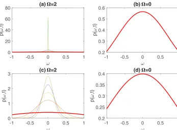
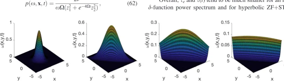
Figures 1(a) and 1(b) compare the time evolution of

p(x,t) forXz¼2 in (a) and forXz¼0 in (b) by usingky¼1,

kx(0)¼0, /¼1, and ¼0.1. The initial PDF is shown in the bottom red curve and the time increases from the bot-tom to the top curve as t_¼0.6n, where n_¼0;1;2;3;

…;10. The narrowing of PDF width in time in Fig.1(a)is in sharp contrast to a much smaller change in Fig. 1(b) between t¼0 and t¼6. A much faster narrowing in Fig. 1(a)manifests the enhanced dissipation of the mean square vorticity byXz.

2. Constant power spectrum

se/Xz2=3 in Eq. (28)is specific to the case of the d -function power spectrum where there is unique wavenumber at t¼0 that evolves according to Eq.(18). To understand howseis affected in the presence of differentk(0) modes, we consider a constant spectrum by taking

w_¼constant_¼/. Then, the power spectrum evolves in time as follows:

w_ðk_ðt_Þ;t_{Þ ¼}e2Q1ðtÞ/; (30)

whereQ1(t) is given in Eq.(19). From Eqs.(23)and(30), we

obtain

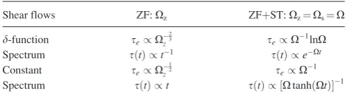
TABLE I. Scalings of se and s(t) for the initial d-function and constant power spectra in the case of ZF with the shearing rateXzand hyperbolic ZFþST with the shearing rateXz¼Xs¼X. Gaussian power spectrum has the scaling betweend-function and constant power spectra.

Shear flows ZF:Xz ZFþST:Xz¼Xs¼X

d-function se_/X23

z se/X1lnX

Spectrum sðtÞ /t1 _{sðtÞ /e}Xt Constant se_/X12

z se/X1

Spectrum s_ðtÞ /t s_ðtÞ / ½XtanhðXtÞ1

FIG. 1. Time evolution of p(x, t) in panels (a) and (b) for the d-function power spectrum in(25)and in panels (c) and (d) for the Gaussian power spectrum in Eq. (A1); t¼0.6n

hx2

ðx;tÞi ¼ p 2t

ffiffiffiffiffiffiffiffiffiffiffiffiffiffiffiffiffiffiffiffiffi 4þ1

3X

2

zt

2

r / (31)

after performing the Gaussian integrals over ky and kx(0). Equation(31)shows thatXzchanges the scaling ofhx2ðx;tÞi fromt1tot2by the enhanced dissipation. In this case,seis found fromXzs2e1 as

se/ ðXzÞ 1

2: ₍₃₂₎

Thus, the dependence of se/Xz1=2 on Xz is weaker than

se/Xz2=3 for a d-function spectrum as the effect of shear-ing is reduced in the case of multiple modes. This is basically because the distortion of an eddy by shearing follows a wave number specific time evolution [e.g., Eq.(18)]; the effect of a shear on multiple modes is not coherent as eddies with dif-ferent wave numbers evolve difdif-ferently and is thus less effective.

This reduced shearing effect can also be inferred fromE in Eq.(12), which becomes

EðtÞ ¼

4þ2 3Xzt

2

2

2t2 _4þ1

3Xzt

2

2: (33)

Thus, Eq. (33) gives the time scale sðtÞ ¼ E1=2

/t for

Xzt1. This should be compared withsðtÞ /t1in the case of a d-function power spectrum above (see Table I). The increase ofs(t) withtmeans a longer time scale of dissipa-tion and thus it manifests that the dissipadissipa-tion becomes less effective for large time. Similar results are shown for the case of an anisotropic power spectrum with kx(0)¼0 in Appendix B. We note that the mean square vorticity in Eq. (31)apparently diverges at t¼0 due to the unlimited range

of the k integral for an initial constant power spectrum. Mathematically, this problem is readily ratified by using a localised spectrum in Sec.IV A 3.

3. Gaussian power spectrum

The initial Gaussian power spectrum w_ð0_{Þ ¼} 1

ap

e1aðkxð0Þ2þk2yÞ_/gives

wðk_ðtÞÞ ¼ 1

ape

1

aðkxð0Þ2þk2yÞ2Q1ðtÞ_/; ₍₃₄₎

where Q1(t) is given in Eq. (19); arepresents the width of

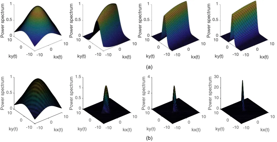
the initial power spectrum;a!0 anda! 1recover thed -function and constant power spectrum, respectively. To understand the effect of Xz on the evolution of w(k(t)) in (34), we usekxð0Þ ¼kxðtÞ Xzkytand presentw(k(t)) in Fig. 2. Without diffusion (¼0), w(k_{(t)) in Fig.2(a) shows the}

generation of large kx wave number due to ZF shearing. When a diffusion (¼0.1) is included in Fig.2(b), largekx (andky) modes quickly damp due to molecular dissipation,

w(k_{(t)) forming a sharp peak aroundkx¼ky¼0.}

On the other hand, using Eqs.(34)and(19)in(23), we find

hx2ðx;tÞi ¼1

a ffiffiffi 1

A

r

/; (35)

where A¼ ð2tþa1_Þ2

þ1

3ðtÞðXztÞ 2

½tþ2a1_{. We note}

that in the limit oft_!0 andt_{! 1}, Eq.(A1)is reduced to

hx2

ðx;tÞit!0 !/; hx 2

ðx;tÞit!1! ffiffiffi 3 p

aXzt2

/; (36)

respectively. The second equation in Eq. (36) recovers the limit of a d-function power spectrum in Eq.(31) (up to an unimportant small numerical factor). Eq. (35) very

FIG. 2. (a) Time evolution of power spectrum (t_¼0, 1, 2, 3 increasing from left to right) forXz¼2,Xs¼0,a¼100,/¼1, and¼0. (b) The same as (a) but for¼0.1.

conveniently shows the transition of the scaling of se from /Xz2=3 in Eq. (28) to /X

1=2

z in Eq. (32) as a increases (see also above).

Figures1(c) and1(d)show the evolution of p(x,t) for this Gaussian power spectrum forXz¼2 andXz¼0, respec-tively. Here, parameter values are the same as those in Figs. 1(a)and1(b)apart from a_¼100. Comparing Fig.1(c)with Fig.1(a), we see much slower narrowing of the PDFs as the shearing effect is less effective in the presence of multiplek

modes. As observed in Figs. 1(a)and1(b), the PDF in Fig. 1(d) for Xz¼0 narrows slower than that in Fig. 1(c). However, comparing Figs. 1(b) and 1(d), the presence of multiple k_{modes tends to promote dissipation (due to high}

wave number modes).

B. Hyperbolic ZF1ST case:X_z>0 andX_s>0

Compared with the case of zonal flows, the combined effect of Zonal Flows and STreamers (ZFþST) has been stud-ied much less. We show below that the action of ZFþST can lead to an exponentially fast formation of small scale struc-ture. For U_{¼ ðyXs;xXzÞ with Xs>0 and Xz>0,} U_has

the mean vorticity r U_{¼ ðXzþXsÞ}^z, which becomes zero forXz¼Xs. The solution to Eq.(18)can be found as

kyðtÞ ¼kX

Xz

coshðXtþh_Þ; kxðtÞ ¼ksinhðXtþhÞ; (37)

where

X¼ ffiffiffiffiffiffiffiffiffiffiXzXs p

; _{k k}

yð0Þ

2

þkxð0Þ

2X2

X2z

" #1₂

; (38)

sinhðhÞ ¼kxð0Þ

k ; coshh¼

Xzkyð0Þ

Xk : (39)

We focus on the case ofXz¼Xs¼Xwith zero mean vortic-ity, in which casek2

xþky2¼k

2

cosh½2ðXtþhÞfollows from Eq.(37). Thus, with the help of Eqs.(38)and(39), we obtain

Q2ðtÞ ¼

Ðt

0dt1jkðt1Þj 2

as

Q2ðtÞ ¼

1

4X½ðkxð0Þ þkyð0ÞÞ

2

ðe2Xt1Þ

þ ðkxð0Þ kyð0ÞÞ2ð1e2XtÞ: (40)

Since k₍t) starting with k_{(0) changes in time according to}

Eq.(37), in order to see how the power spectrum evolves in time, we need to expressQ2(t) in Eq.(40)in terms of k(t).

To this end, we solve Eq. (37) for kx(0) and ky(0) to find

kyð0Þ ¼ kyðtÞcoshðXtÞ kxðtÞsinhðXtÞ and kxð0Þ ¼ kxðtÞ coshðXt_Þ kyðtÞsinhðXtÞ, and thus

kxð0Þ þkyð0Þ ¼ kxðtÞ þkyðtÞeXt;

kxð0Þ kyð0Þ ¼ kxðtÞ kyðtÞeXt:

(41)

By using Eq.(41)in Eq.(40), we have

Q2ðtÞ ¼

1

4X½ kxðtÞ þkyðtÞ 2

ð1e2Xt_Þ

þ kxðtÞ kyðtÞ 2

ðe2Xt1Þ: (42)

Interestingly, Eq.(42)shows that the dissipationQ2(t) takes

its minimum value whenkx(t)¼ky(t). Furthermore, from Eq. (41), we also find

kxð0Þ2þkyð0Þ2¼ 1

2½ðkxðtÞ kyðtÞÞ

2

e2Xt

þ ðkxðtÞ þkyðtÞÞ2e2Xt; (43)

which also takes its minimum alongkx(t)¼ky(t). The minimum of Eqs.(42)and(43)alongkx(t)¼ky(t) is later shown to give a peak in the power spectrumw(k(t)) in Sec.V(see Fig.3). We refer tokx(t)¼ky(t) as the principle direction in the following.

1.d-function power spectrum

For ad-function power spectrum given by Eq.(25), the power spectrumw(k₍t)) continues to have a d-function with the peak at kx(t) and ky(t) given by Eq.(37) with kx(0)¼a andky(0)¼b. This leads to

hx2ðx_{;tÞi ¼exp}

2X½ðkxð0Þ þkyð0ÞÞ

2

ðe2Xt1Þ

ðkxð0Þ kyð0ÞÞ2ðe2Xt1Þ

/: (44)

From Eq.(44), we find the effective diffusion timese

se 1 2Xln

2X jk_0j2

!

: (45)

sein Eq.(45)is smaller than Eq.(28)for a sufficiently large

X, with a stronger dependenceX1lnXonX, in comparison withXz2=3 in ZF case. Furthermore, due to the double expo-nential decrease in_hx2

i;s_ðt_Þin Eq.(12)is reduced exponen-tially fast as

sðtÞ /eXt: (46)

The exponentially decreasings(t) in Eq.(46)reflects a very efficient dissipation by ZFþST. The evolution of PDF is shown in Fig. 3for X¼2 in (a) and X¼0 in (b). The time

t_¼0.2n, wheren_¼0, 1, 2, 3, 4, and 5 increases from the bottom to the top curves. The bottom red curve is for the ini-tial PDF. Comparing Fig.3(a)with Fig.1(a), we see a much faster narrowing of the PDFs in the hyperbolic ZFþST case due to a much faster dissipation. (Note that the total time span

t¼[0, 1] in Fig.3is much smaller thant¼[0, 6] in Fig.1.) The change in Fig.3(b)withX¼0 is too small to be seen.

2. Constant power spectrum

For an initial constant power spectrum w(0)¼/, the power spectrum again evolves as wðk_ðtÞ;tÞ ¼e2Q2ðtÞ_/, whereQ2is given in Eq.(40). Therefore, by using Eqs.(23)

and(40), we find

hx2ðx;tÞi ¼1 2 ð

dpdqexp

2X p

2

ðe2Xt1Þ þq2ð1e2XtÞ

/

¼ X/

Here, we performed the integrals overpkx(0)þky(0) and

qkx(0) –ky(0).

Compared with the d-function power spectrum, the effect of shear flow is reduced from double exponential to exponential. For Xt1;hx2

ðx;t_Þi X

2peXt/, giving an effective diffusion time

seX1: (48)

Interestingly,s(t) in this case has a similar dependence onX

since

sðtÞ ¼ 1

XtanhðXt_Þ; (49)

approaching a constant valueX1(!) fort X1. This is another example of a geodesic, which is more interesting than the case of Xz¼0 in Eq. (29) because Eq. (49) is induced by non-zero X in the presence of different k(t) modes which evolve from an initial constant power spec-trum. In fact,s(t)X1explicitly shows thatXis the very cause of information change. On the other hand, in compari-son with the exponentially decreasing s(t) in Eq. (46), Eq. (49) again illustrates the reduced shearing effect due to the presence of multiple k _{modes. Finally, we note that the}

divergence att¼0 is due to the unbounded power spectrum as in the case of Eq.(31). Scalings ofseands(t) are summa-rized in TableI.

3. Gaussian power spectrum

Forw_ð0Þ ¼ 1

ape

1

aðkxð0Þ2þkyð0Þ2Þ_{/, we have}

wðk_ðtÞÞ ¼ 1

ape

1

aðkxð0Þ2þkyð0Þ2Þ2Q2ðtÞ_{/; (50)}

whereQ2is given by Eq.(40). By using Eqs.(42)and(43)

in Eq.(50), we present the evolution of the power spectrum

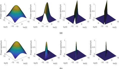
w(k(t)) in Fig.4forX¼2, where time increases from left to right as t_¼0, 0.6, 1.2, and 1.8. Without diffusion (¼0),

w(k_{(t)) in Fig.4(a) shows a fast reduction in} w(k_{(t)) along}

kx(t)þky(t)¼0, with the peak forming along the principle direction kx(t)¼ky(t). When diffusion (¼0.1) is included in Fig. 4(b), modes of large wavenumber also damp along the principle direction in time due to the molecular dissipa-tion although the damping is weaker compared to that along

kx(t)þky(t)¼0. This is because the dissipation Q2(t) in Eq.

(42) and kx(0)2þky(0)2 in Eq. (43) are minimized along

kx(t)¼ky(t), as noted previously.

Now, Eq.(50)leads to the mean square vorticity

hx2ðx;tÞi ¼ 2

ap ð

dpdqexp

2X

p2ðe2Xt1Þ

þq2ð1e2XtÞ 1

aðp

2

þq2Þ

/

¼ 2

a ffiffiffiffiffiffi

AB

p ; (51)

where

A¼ 2Xðe

2Xt_{1Þ þ}1

a; B¼

2Xð1e

2Xt_{Þ þ}1

a: (52)

se/X1is thus similar to Eq.(48)fort X1. However, in contrast to Eq. (49),s(t) becomes constant fort X1

only for a sufficiently largea, that is, in the limit of a con-stant power spectrum. Figure 3(c) shows the evolution of

p(x, t) for this case using the same parameter values

Xz¼Xs¼X¼2 as in Fig. 3(a) apart from a¼100. Comparing Fig.3(c)with Fig.3(a), we see much slower nar-rowing of the PDFs as the shearing effect is less effective in the presence of multiplek_{modes, as observed in Fig.1. The}

evolution of p(x,t) for X¼0 is shown in Fig. 3(d), which hardly changes.

FIG. 3. Time evolution ofp(x,t) for thed-function power spectrum in Eq. (44)in panels (a) and (b) and for the Gaussian power spectrum in Eq.(51) in panels (b)–(d); t_¼0.2n, where

n_¼0, 1, 2, 3, 4, 5 increases from the bottom to the top curves. The bottom red curve is for the initial PDF. a_¼100,¼0.1, and/_¼1.

C. Elliptic ZF1ST case

For the hyperbolic ZFþST case in Sec.IV B, the sign of zonal flow and streamer shear is the same. When they have different signs, ZFþST leads to a rotating wave number. To see this, we consider U_{¼ ð}yXs;xXzÞ with Xs>0 and

Xz>0 which has the nonzero mean vorticity r U ¼ ðXzþXsÞ^z. For this ZFþST, we find the solution to Eq. (18) as kyðtÞ ¼k_XX_zcosðXtþhÞ and kxðtÞ ¼ksinðXtþhÞ,

where X¼ ffiffiffiffiffiffiffiffiffiffi XzXs p

;k_{¼ ½}kxð0Þ

2

þkyð0Þ

2X2

z X2

1

2_{, and sinðhÞ}

¼kxð0Þ

k ; cosh¼

Xzkyð0Þ

Xk . WhenXz¼Xs¼X;k

2

xþk

2

y¼kxð0Þ2 þkyð0Þ

2

is a constant in time, with no enhancement of dissi-pation. However, for Xz6¼Xs, kx2þk2y¼k

2

½sin2ðXtþhÞ þXs

Xzcos

2_ð

XtþhÞ. Although the overall dissipation may not be significantly enhanced by this shear flow, there is an inter-esting effect on the dynamics due to oscillatory dissipation,

kxorky, which provides a periodic background (or potential). This is discussed in our accompanying paper.34

V. NON-GAUSSIAN PDFs

In Sec.IV, we investigated the effect of shear flows on the evolution of the Gaussian PDFs and power spectra. The main effect was the shift of power to larger wavenumber, accelerating dissipation, and narrowing PDF width. We now extend our study to a non-Gaussian case to examine the effect of shear flows on the form of PDF. Although there are many possible causes for non-Gaussian PDFs, we consider one example of an inhomogeneous turbulence. That is, we drop the assumption of homogeneous turbulence and instead prescribe the profile of the initial vorticity fluctuation as

~

x_ðk_{ð0Þ;t¼0Þ ¼} 1

ape

1

aðkxð0Þ2þkyð0Þ2Þ_;

xðx;t¼0Þ ¼ea4ðx 2_þy2_Þ

;

(53)

whereais a positive random variable. Note that whena_¼0, Eq.(53)gives a constantx(x_{, 0) while the nonzero constanta}

(>0) gives the typical length scalelof the profile of the initial vorticity fluctuation asla1=2

. A random positiveamakes the profile of the initial vorticity fluctuation on different length scales. By considering the hyperbolic shear flow considered in Sec.IV B, we have

~

x_ðk_ðt_Þ;t_{Þ ¼} 1

ape

1

aðkxð0Þ2þkyð0Þ2ÞQ2ðtÞ_{; (54)}

whereQ2(t) is given in Eq.(40). In order to take the inverse

Fourier transform of Eq. (54) to findx(x, t), we first write Eq. (37) in terms ofp¼kx(0)þky(0) andq¼–kx(0)þky(0) as kyðtÞ ¼12½peX

t_þqeXt _{and k}

xðtÞ ¼12½peX

t_qeXt _so that

k_ðtÞ x_¼1

2 pe

Xt_z

1þqeXtz2

; (55)

where

z1¼xþy; z2¼yx: (56)

Then, by using Eqs. (40), (54), and (55), we obtainx_ðx_;t_Þ

¼Ð

dk_ðtÞeik_ðtÞx ~

x_ðk_ðtÞ;tÞas

x_ðx_;t_{Þ ¼} 1

2a ffiffiffiffiffiffiffi

CD

p exp e

2Xt_z2 1

8C e2Xt_z2

2

8D

: (57)

Here

C¼ 4Xðe

2Xt_{1Þ þ} 1

2a; D¼

4Xð1e

2Xt_{Þ þ} 1 2a: (58)

Ast!0;C! 1 2a; D!

1

2a, and Eq.(57)recovers Eq.(53).

Fort6¼0,CandDdepend on the relative magnitude of 4/X

and 1/2a.

Before proceeding to randoma, we note that for a con-stant value of a, Eq. (57) shows the anisotropic distortion and decay of the profile of vorticity fluctuation by shear flows. The time evolution ofx(x_{,t) for constanta¼100 is}

shown in Fig. 5, where time t¼0, 5, 1, and 1.5 increases from left to right. Of notable is the flattening and elongation of x(x, y, t) along z1¼xþy¼0, with the formation of a

sheet like structure. This is quite similar to what is seen in Fig. 4, recalling that a narrow k profile corresponds to a broadx_profile.

Whena(>0) is random, the statistics ofx(x_{,t) depends}

onaas

pðx;x;tÞ ¼

da

dx

pðaÞ: (59)

In particular, att¼0, Eq. (53)givesa¼ 4ln ðxðt¼0ÞÞ=

r2_{, wherer}2

¼x2þy2, leading to

p_ðx;x_{;0Þ ¼} 4

xr2pðaÞ: (60)

For our purpose, it suffices to assume thatais uniformly distributed within a certain range. Two cases of our interest are the limit of weak inhomogeneity, where (i) a_{¼ ½}0;2X

e

2Xt

and of a strong inhomogeneity and (ii) a_{¼ ½}2X

;ac with

ac>2X. In case (i), the shearing does not have much influence on the scale of inhomogeneity, while in case (ii), it does have a significant effect. Starting our analysis in case (i), we approxi-mateCD 1

2a, and consequently

xðx_{;tÞ exp} a

4 e

2Xt_z2 1þe

2Xt_z2 2

¼exp a 4G1

;

(61)

where G1 ¼e2Xtz21þe2Xtz22. Eqs. (59) and (61) will then

give us

pðx;x_{;tÞ ¼} 2

xXðz2

1þe4Xtz 2 2Þ

; (62)

for a<2X

e

2Xt_{. In Eq. (62), we used pðaÞ ¼}e2Xt

2X for a¼ ½0;2X

e

2Xt_{. A rapid decrease of p(x,x,t) in Eq. (62)} for largez2

1is similar to the elongation of the vorticity profile

alongz2, observed in Fig.5. We note here that the condition

on a<2X

e

2Xt _{is translated into xðx;tÞ>exp½}XG1

2 e

2Xt

exp½X 2ðz

2

1þe4Xtz22Þ:

The case (ii) where a¼ ½2X

;ac, we have xðx;tÞ 2X

aeXtG2, whereG2¼₂Xðz21þe 2Xt_z2

2Þ. Thus,

pðx;x_{;tÞ /} 2X

ax2e

XtG2_{; (63)}

forx_{¼ ½}2X

ace

XtG2_;eXtG2_{, becoming very small for large}

z2

1. Compared with Eq.(60)or(62),p(x,x,t)/x

2

in Eq. (63)drops more rapidly for largex. Interestingly, this is sim-ilar to the narrowing of Gaussian PDFs by shear flows shown in Sec.IV. Finally, going back to our discussion on the PDF method in Sec. II, we can compute the first three terms in Eq. (5) using our p(x, x, t) above to realize that a correct form of the last term in Eq.(5)is quite complicated and non-linear inp(x,x,t), as noted in Sec.II. The diffusion term in Eq. (1) cannot be simply neglected and needs to be treated very carefully.

VI. DISCUSSION AND CONCLUSIONS

We have presented the first analytical study of the effects of shear flows on enhanced dissipation in a decaying turbulence in 2D by incorporating the effects of shear flows non-perturbatively. We considered different initial power spectra and shear flows (ZF, ZFþST) and clearly demon-strated how shear flows induce the rapid formation of small scales (large wave number modes), significantly enhancing the dissipation of turbulence. We presented time-dependent PDFs and discussed the effects of enhanced dissipation by shear flows on PDFs and effective dissipation time scalese. While previous works advocated a hybrid time scale se /X2=3sg(e.g., Ref.16), wheresgis the time scale due to a

molecular diffusion, we showed that the dependence ofseon

X (Xz) varies with initial power spectra and also types of shear flows. In addition, we demonstrated the utility of a dynamical time scale s(t) in understanding the effect of shears, which quantifies the rate of the change in information (the rate at which a system passes through statistically differ-ent states).

Overall,seands(t) tend to be much smaller for an initial

d-function power spectrum and for hyperbolic ZFþST. ZF

FIG. 5. Time evolution ofx(x,y,t) forXz¼Xs¼X¼2,t¼0, 0.5, 1, 1.5 increasing from left to right;a¼2,¼0.1, and/¼1.

can dramatically reduces(t) for an initiald-function power spectrum but not for a constant power spectrum. This was however obtained in the case where the mean vorticityhxTi is independent of time.35 A time-varying hxTi ¼ Xz, which is more likely in real situations (e.g., time-varying zonal flows), would however make s(t) very small (see Appendix C), with interesting consequences to be investi-gated. Finally, hyperbolic ZFþST was shown to cause an exponential increase in wavenumber, with a double exponen-tial decrease inhx2_i.

The preferential dissipation by shear flows in a certain direction can lead to a strongly anisotropic turbulence, as also shown in Refs.7–9(with a possibility of the reduction in dimension), in analogy to the maintenance of a 2D flow in a forced 3D rotating turbulence.36In 3D, the vortex stretch-ing (which is absent in 2D) could somewhat compensate the severe quenching of vorticity amplitude. However, for a lin-ear shlin-ear flow U_{¼ xX}y^, Eq. (D14) in Appendix D (see also Ref.8) shows that the Fourier components of the veloc-ity damp in time as~v_x/t2eQðt;0Þ;~v_z/eQðt;0Þ, and~v_y/

eQðt;0_Þ

to leading order for t>kxð0Þ

kyX. Here, Qðt;0Þ

¼1 3ðkyXÞ

2

t3

þkykxð0ÞXt2þ ½kxð0Þ

2

þk2

yþk

2

zt. Therefore, in addition to the enhanced dissipation e–Q(t,0)through the time-dependent wave number, v_x undergoes the additional algebraic (/t2) quenching. The vorticity fluctuationx~_would

then be at most/te–Q(t,0)inyandzdirections. Investigation of the effect of different shear flows on 3D turbulence, the extension to different models such as interchange turbu-lence,34magnetic dissipation, and dynamos, and implications for extreme events37are left for future work.

APPENDIX A: RELATION BETWEENL_{AND RELATIVE} ENTROPY

We first show the relation between s(t) in Eq.(10)and the second derivative of the relative entropy (or Kullback-Leibler divergence) Dðp1;p2Þ ¼Ðdx p2lnðp2=p1Þ, where

p1¼p(x,t1) andp2¼p(x,t2) as follows:

@ @t1

D_ðp1;p2Þ ¼

ð

dxp2

@t1p1

p1

; (A1)

@2

@t2 1

Dðp1;p2Þ ¼

ð

dxp2 ð

@t1p1Þ2

p2 1

@

2

t1p1

p1

" #

; (A2)

@ @t2

D_ðp1;p2Þ ¼

ð

dx @t2p2þ@t2p2ðlnp2lnp1Þ

; (A3)

@2

@t2 2

Dðp1;p2Þ ¼

ð

dx @2

t2p2þð

@t2p2Þ2

p2 þ

@2

t2p2ðlnp2lnp1Þ

" #

:

(A4)

By taking the limit wheret2!t1¼t(p2!p1¼p) and by

using the total probability conservation (e.g., Ð

dx@tp¼0), Eqs.(D3)and(D5)lead to

lim t2!t1¼t

@ @t1

Dðp1;p2Þ ¼ lim

t2!t1¼t

@ @t2

Dðp1;p2Þ ¼

ð

dx@tp¼0;

while Eqs.(D4)and(D6)give

lim t2!t1¼t

@2

@t2 1

Dðp1;p2Þ ¼ lim

t2!t1¼t

@2

@t2 2

Dðp1;p2Þ ¼

ð

dxð@tpÞ

2

p :

To link this to information length L, we then express

D(p1,p2) for smalldt¼t2–t1as

Dðp1;p2Þ ¼

ð

dxð@t1pðx;t1ÞÞ

2

p

" #

ðdtÞ2þOððdtÞ3Þ; (A5)

where O((dt)3) is a higher order term in dt. We define the infinitesimal distance (information length) dl(t1) betweent1

andt1þdtby

dlðt1Þ ¼

ffiffiffiffiffiffiffiffiffiffiffiffiffiffiffiffiffiffi

Dðp1;p2Þ

p

¼

ffiffiffiffiffiffiffiffiffiffiffiffiffiffiffiffiffiffiffiffiffi ð

dxð@tpÞ

2

p

s

dtþOððdtÞ3=2Þ: (A6)

The total change in information between time 0 andtis then obtained by summing overdt(t1) and then taking the limit of

dt!0 as

Lðt_{Þ ¼} lim

dt!0½dlð0Þ þdlðdtÞ þdlð2dtÞ þdlð3dtÞ þ dlðtdtÞ

¼ lim dt!0

ffiffiffiffiffiffiffiffiffiffiffiffiffiffiffiffiffiffiffiffiffiffiffiffiffiffiffiffiffiffiffiffiffiffiffiffiffi

D_ðp_ðx;0_Þ;p_ðx;dt_ÞÞ

p

þpDffiffiffiffiffiffiffiffiffiffiffiffiffiffiffiffiffiffiffiffiffiffiffiffiffiffiffiffiffiffiffiffiffiffiffiffiffiffiffiffi_ðp_ðx;dt_Þ;p_ðx;2dt_ÞÞ

þ ffiffiffiffiffiffiffiffiffiffiffiffiffiffiffiffiffiffiffiffiffiffiffiffiffiffiffiffiffiffiffiffiffiffiffiffiffiffiffiffiffiffiffi

Dðpðx;tdtÞ;pðx;tÞÞ p / ðt 0 dt1 ffiffiffiffiffiffiffiffiffiffiffiffiffiffiffiffiffiffiffiffiffiffi ð

dxð@t1pÞ

2

p

s

: (A7)

APPENDIX B: ANISOTROPIC CONSTANT POWER SPECTRUM

To demonstrate an incoherent shearing effect in the presence of multiple modes, it is interesting to consider an isotropic power spectrum by keeping a constant spectrum in

kybut takingkx(0)0. The mean square vorticity is obtained from Eq.(31)by takingkx(0)!0, with the result

hx2_ðx;t_{Þi ¼}

ffiffiffiffiffiffiffiffiffiffiffiffiffiffiffiffiffiffiffiffiffiffiffiffiffiffiffiffiffiffiffiffiffiffi p

2t 1þ1 3X 2 zt 2 v u u u t

/: (B1)

Thus, hx2

ðx;t_{Þi /}t3=2

, decreasing less rapidly than hx2

ðx;t_{Þi /}t2

in Eq.(31). On the other hand, the effective dissipation timeseis similar to Eq.(32).

APPENDIX C: SLOWLY TIME-VARYING ZF

We assumeXz¼Xz0et=s0andkx00. Then, we have

kxðtÞ ¼ ðt

0

dt1kyXzðt1Þ ¼kyXz0s0ð1et=s0Þ; (C1)

Q1ðtÞ ¼ ðkyXz0s0Þ2

s0

3 1e t=s0 ½ 3_þk2_yt

1 3ðkyXz0Þ

2

@tXz 1

s0X

z0; (C3)

fort s0. Thus, Eqs.(12),(31), and(33)with the help of Eqs.(C2)and(C3)give us

E ¼ 1

sðtÞ2¼ 1 2

ð@tbÞ2

b2 þ2bð@tXzÞ

2

4þ2 3Xzt

2

2

2t2 _4þ1

3Xzt

2

2þ

2t

ffiffiffiffiffiffiffiffiffiffiffiffiffiffiffiffiffiffiffiffiffiffi 4þ1

3Xz0t

2

r

p/s2 0

X2z0: (C4)

The second term is due to the change ofXzmeasured in the unit of the very small PDF width /b12/ hx2i

1

2_{. As time} increases, the second term obviously makes a significant contribution.

APPENDIX D: 3D HYDRODYNAMIC TURBULENCE

In 3 D, the main governing equations for the total veloc-ityu_¼v_þU_are8

@tuþu ru¼ rpþr2uþf; (D1)

r u_{¼0; (D2)}

where f _{is a small scale forcing in general. By using}

U_{¼ xX}^y,

@t^v_x¼ ik_xp^þf^

x; (D3)

@t^v_yX^v_x¼ ik_yp^þf^

y; (D4)

@t^v_z¼ ik_zp^þf^

z; (D5)

0¼kx^v_xþk_y^v_yþk_z^v_z; (D6)

where the second term in Eq. (D4) is due to the vortex stretching. Here,w^andw~forw¼vi,p, andfare defined as

w_ðx_;t_{Þ ¼}w~_ðk_;t_Þexpfi_ðkxðtÞxþkyyþkzzÞg; (D7)

^

ww~expfðk3_x=3kyXþkH2tÞg; (D8)

where k2

H¼k2yþk2z;kxðtÞ ¼kxð0Þ þXkyt. Now, to solve coupled equations(D3)–(D6), we introduce a new time vari-ables¼kx/kyþXtand rewrite them as

X@s^v_x¼ isk_yp^þf^

x; (D9)

X@s^v_yX^v_x¼ ik_yp^þf^

y; (D10)

X@s^v_z¼ ik_zp^þf^

z; (D11)

0¼s^v_xþk_y^v_yþkz

ky

^v_z: (D12)

A straightforward, but rather long, algebra then gives us the solutions in the following form:

^

v_xðsÞ ¼ 1

cþs2

ðs

ds1h1ðs1Þ;

^v_zðsÞ ¼ ðs

ds1

~ b s1 ^ v_x ~ b s1 ^

f_xþf^_z

" #

;

¼ ~bs

c ^vxþ ðs

ds1

1

c

h2ðs1Þ

~ b c1=2 tan

1 s

ffiffiffi c

p tan1 s1_ffiffiffi

c

p

h1ðs1Þ

" #

;

^

v_yðsÞ ¼ s^v_xðsÞ b~u^v_zðsÞ;

^

p_¼X kyð

@s^v_xþf^

xÞ; (D13)

where ~b_¼kz=ky;c¼1þb~

2

;h1¼ ð1þb~ 2

Þf^_xsf^_ysb~f^_z, andh2¼ ~bf^yþf^z. Finally, going back to the original vari-ablekx¼kys, we obtain

~

v_xðkðtÞ;tÞ ¼ ð

dt1d3k1

k2

y

k2g^ðk;t;k1;t1Þe

Qðt;t1Þ_h~_1ðk₁;x;t1Þ;

~v_zðkðtÞ;tÞ ¼ kxkz

k2

H

~v_xðkðtÞ;tÞ þ ð

dt1d3k1g^ðk;t;k1;t1Þ

eQðt;t1Þh~2ðk1;x;t1Þ

k 2 y k2 H ~

h2ðk1;x;t1Þ

kzk2y jk3

Hj "

tan1 kx jkHj

tan1 k1x jk1Hj

~

h1ðk1;x;t1Þ

;

~

v_yðkðtÞ;tÞ ¼ kx

ky

~

v_xðkðtÞ;tÞ kz

ky

~

v_zðkðtÞ;tÞ: (D14)

Here, Q_ðt;t1Þ ¼

Ðt t1dt0½k

2

xðt0Þ þk

2

H ¼ ½k

3

xk

3

1x=3kyXþkH2 ðtt1Þ; k_H2 ¼k_y2þk2_z;k2¼ k_H2 þk2_x; ^gðk;t;k1;t1Þ ¼dðky k1yÞdðkzk1zÞd½kxk1xk1yðtt1ÞX;h~1¼ ð1þk2_z=k_y2Þf~x kxf~y=kykxkzf~z=k2y; ~h2¼ kzf~y=kyþf~z. By taking f~iðt1Þ

¼~v_iðt₁Þdðt₁Þ, we obtain the homogeneous solution without the forcing.

1_{K. H. Burrell,Phys. Plasmas4, 1499 (1997).}

2_{T. S. Hahm, Plasma Phys. Controlled Fusion44, A87 (2002);1,2940}

(1994);2_,1648(1995).

3_{M. Dam, M. Brons, J. J. Rasmussen, V. Naulin, and J. S. Hesthaven,Phys.} Plasmas24_{, 022310 (2017).}

4

C. S. Chang, S. Ku, G. R. Tynan, R. Hager, R. M. Churchill, I. Cziegler, M. Greenwald, A. E. Hubbard, and J. W. Hughes,Phys. Rev. Lett.118, 175001 (2017).

5

E. Kim and P. H. Diamond,Phys. Rev. Lett.91_{, 075001 (2003); E. Kim,} Mod. Phys. Lett. B18, 551 (2004).

6

E. Kim,Phys. Rev. Lett.96_{, 084504 (2006); E. Kim and B. Dubrulle,} Phys. Plasmas8, 813 (2001).

7_{E. Kim,Astron. Astrophys.441, 663 (2005).}

8_{E. Kim and N. Leprovost, Astron. Astrophys. 456, 617 (2006); N.}

Leprovost and E. Kim,Astron. Astrophys. Lett.463_{, L9 (2007); E. Kim} and N. Leprovost,Astron. Astrophys.465, 633 (2007); N. Leprovost and E. Kim,Astron. Astrophys.468_{, 1025 (2007).}

9

E. Kim,Phys. Plasmas 12, 090902 (2005); E. Kim,Phys. Plasmas13, 022308 (2006); E. Kim and P. H. Diamond,Phys. Plasmas11, L77 (2004).

10

J. Li and Y. Kishimoto,Phys. Plasmas11_{, 1493 (2004).}

11

Y. Idomura, S. Tokuda, and Y. Kishimoto,Nucl. Fusion45_{, 1571 (2005).}

12_{X. U. Guosheng and W. U. Xingquan,Plasma Sci. Technol.19, 033001}

(2017).

13_{E. J. Synakowski, S. H. Batha, M. A. Beer, M. G. Bell et al., Phys.} Plasmas4_{, 1736 (1997).}

14_{X. Garbet,Plasma Phys. Controlled Fusion43, A251 (2001).}

15_{G. Rewoldt, M. A. Beer, M. S. Chance, T. S. Hahmet al.,Phys. Plasmas}

5_{, 1815 (1998).}

16_{P. H. Diamond, S.-I. Itoh, K. Itoh, and T. S. Hahm, Plasmas Phys.} Controlled Fusion47_{, R35 (2005); P. H. Diamond, A. Hasegawa, and K.} Mima,ibid.53, 124001 (2011).

17_{M. E. McIntyre,J. Atmos. Terr. Phys.51, 29 (1989).} 18

J. C. R. Hunt and P. A. Durbin,Fluid Dyn. Res.24_{, 375 (1999).}

19

A. Sood, E. Kim, and R. Hollerbach,J. Phys. A: Math. Theor.49_{, 425501} (2016).

20_{A. P. Newton and E. Kim,Phys. Plasmas18, 052305 (2011).} 21

S. B. Pope,Turbulent Flows(Cambridge University Press, 2000).

22

J. Zinn-Justin,Quantum Field Theory and Critical Phenomena(Clarendon Press, 2002).

23

H. Risken, The Fokker-Planck Equation: Methods of Solution and

Applications(Springer, Berlin, 1996).

24_{S. B. Nicholson and E. Kim,Phys. Lett. A379, 83–88 (2015).} 25

S. B. Nicholson and E. Kim,Entropy18_{, 258 (2016).}

26_{J. Heseltine and E. Kim, J. Phys. A: Math. Theor. 49, 175002}

(2016).

27

E. Kim, U. Lee, J. Heseltine, and R. Hollerbach,Phys. Rev. E93_{, 062127} (2016).

28

E. Kim and R. Hollerbach,Phys. Rev. E95, 022137 (2017).

29_{R. Hollerbach and E. Kim,Entropy19(6), 268 (2017).}

30_{B. R. Frieden, Physics from Fisher Information(Cambridge University}

Press, Cambridge, 2000).

31_{W. K. Wootters,Phys. Rev. D23, 357 (1981).} 32

G. Ruppeiner,Phys. Rev. A20_{, 1608 (1979).}

33

F. Schl€ogl, Z. Phys. B - Cond. Matt.59_{, 449 (1985).}

34

I. Movahedi and E. Kim, “Effects of shear flows on the evolution of fluctu-ations in interchange turbulence,” Phys. Plasmas (to be published); arXiv:1711.04897.

35

In such a case,s(t)essentially measures the rate of change in the differen-tial entropy/ Ð

dxplnp¼1 2½1lnð

b

pÞfor a Gaussian PDF in Eq.(11). 36_{B. Gallet,J. Fluid Mech.783, 412 (2015).}

37