JHEP04(2016)023
Published for SISSA by SpringerReceived: October 14, 2015 Revised: February 5, 2016 Accepted: March 2, 2016 Published: April 5, 2016
Search for anomalous couplings in the
W tb
vertex
from the measurement of double differential angular
decay rates of single top quarks produced in the
t
-channel with the ATLAS detector
The ATLAS collaboration
E-mail: atlas.publications@cern.ch
Abstract: The electroweak production and subsequent decay of single top quarks is
de-termined by the properties of theWtb vertex. This vertex can be described by the complex
parameters of an effective Lagrangian. An analysis of angular distributions of the decay
products of single top quarks produced in the t-channel constrains these parameters
si-multaneously. The analysis described in this paper uses 4.6 fb−1 of proton-proton collision
data at √s= 7 TeV collected with the ATLAS detector at the LHC. Two parameters are
measured simultaneously in this analysis. The fractionf1of decays containing transversely
polarised W bosons is measured to be 0.37±0.07 (stat.⊕syst.). The phase δ− between
amplitudes for transversely and longitudinally polarised W bosons recoiling against
left-handedb-quarks is measured to be −0.014π±0.036π (stat.⊕syst.). The correlation in the
measurement of these parameters is 0.15. These values result in two-dimensional limits
at the 95% confidence level on the ratio of the complex coupling parameters gR and VL,
yielding Re[gR/VL]∈[−0.36,0.10] and Im[gR/VL]∈[−0.17,0.23] with a correlation of 0.11.
The results are in good agreement with the predictions of the Standard Model.
JHEP04(2016)023
Contents1 Introduction 1
2 Measurement definition 3
3 The ATLAS detector 6
4 Data and simulated samples 7
5 Object definitions and event selection 8
6 Background estimation and event yields 10
7 Analysis method 11
8 Sources of systematic uncertainty 17
8.1 Object modelling 17
8.2 MC generators and PDFs 17
8.3 Signal and background normalisation 18
8.4 Detector correction and background parameterisation 18
8.5 Uncertainty combination 18
9 Results 18
10 Conclusion 21
A Parameter dependence of the folding and background models 23
The ATLAS collaboration 29
1 Introduction
The top quark is the heaviest known fundamental particle, making the measurement of its production and decay kinematics a unique probe of physical processes beyond the Standard
Model (SM). The top quark was first observed in 1995 at the Tevatron [1, 2] through its
dominant production channel, top-quark pair (t¯t) production via the flavour-conserving
strong interaction. An alternative process produces single top quarks through the weak
interaction, first observed at the Tevatron in 2009 [3,4].
The t-channel exchange of a virtual W boson is the dominant process contributing to
JHEP04(2016)023
q′
W+
b
t
ℓ+
ν
W+
b q
(a)
q′
W+
b t
ℓ+
ν W+
b ¯
b g
q
[image:3.595.130.465.91.238.2](b)
Figure 1. Representative Feynman diagrams fort-channel single top-quark production and decay. Hereqrepresents auor ¯dquark, andq0 represents ador ¯uquark, respectively. The initialb-quark
arises from (a) a sea b-quark in the 2 → 2 process, or (b) a gluon splitting into a b¯b pair in the 2→3 process.
proton-proton (pp) collisions at√s= 7 TeV using a next-to-leading-order (NLO) QCD
pre-diction with resummed next-to-next-to-leading logarithmic (NNLL) accuracy, referred to as approximate next-to-next-to-leading order (NNLO). With a top-quark mass of 172.5 GeV and MSTW2008NNLO[5] parton distribution function (PDF) sets, the cross-section for
the t-channel process is calculated to be 64.6+2−1..67 pb [6]. The uncertainties correspond
to the sum in quadrature of the error obtained from the MSTW PDF set at the 90% confidence level (C.L.) and the factorisation and renormalisation scale uncertainties.
New physics resulting in corrections to the Wtb vertex would affect t-channel single
top-quark production and decay, and can be probed through processes which affect vari-ables sensitive to the angular distributions of the final-state particles from the top-quark decay. Within the effective field theory framework, the Lagrangian can be expressed in full
generality as [7,8]:
LWtb =− g
√
2bγ
µ(V
LPL+VRPR)tWµ−− g
√
2b
iσµνq ν
mW
(gLPL+gRPR)tWµ−+ h.c., (1.1)
wheregis the weak coupling constant, andmW andqν are the mass and the four-momentum
of theW boson, respectively. PL,R ≡(1∓γ5)/2 are the left- and right-handed projection
operators and σµν = i[γµ, γν]/2. V
L,R and gL,R are the complex left- and right-handed
vector and tensor couplings, respectively. The couplings could also be expressed using the
Wilson coefficients [9] of the relevant dimension-six operators,1 described in refs. [7, 10].
In the SM at tree level,VL=Vtb, which is an element in the Cabibbo-Kobayashi-Maskawa
(CKM) matrix, while the anomalous couplings VR = gL,R = 0. Deviations from these
values would provide hints of physics beyond the SM, and complex values could imply that
top-quark decay has a CP-violating component [11].
1In general the couplings can depend on the momentum transferq2. Since this analysis is mainly sensitive
to top-quark decays to an on-shellW boson, whereq2=m2
JHEP04(2016)023
Indirect constraints on VR,gL, and gR were obtained [12,13] from precision
measure-ments of B-meson decays. These result in very tight constraints on VR and gL, but much
looser constraints on gR. Calculations of the anomalous couplings in specific models
pre-dict a much larger contribution to gR than to VR orgL [14]. However, within the models
studied so far for tensor couplings, the magnitude of gR is expected to be <0.01 [14,15].
Measurements of the W boson polarisation fractions [16–19] are sensitive to the
magni-tude of combinations of anomalous couplings. In order to obtain constraints on Re [gR] in
those measurements, the anomalous couplings are taken to be purely real, VR = gL = 0
is assumed and VL is fixed to 1. In this analysis, the anomalous couplings VL and gR are
allowed to be complex, and the ratios Re [gR/VL] and Im [gR/VL] are measured.
This paper is organised as follows. Section 2 describes the coordinate system and
pa-rameterisation used in the measurement. Section3gives a short description of the ATLAS
detector, then section 4 describes the simulated samples used to predict properties of the
t-channel signal and the background processes, and the data samples used. Section 5
describes the definitions of the objects used to identify t-channel events, and the set of
criteria applied to reduce the number of background events. The procedures for modelling
background processes are described in section 6, along with comparisons between the
pre-dictions and data. Section 7 describes the efficiency, resolution, and background models
used to translate the distribution of truet-channel signal events to the distribution of
recon-structed signal and background events, and how the parameters of the model are estimated.
Section 8 quantifies the sources of uncertainty important in this measurement, section 9
presents the resulting central value and covariance matrix for the model parameters and
the ratios Re [gR/VL] and Im [gR/VL], and the conclusions are given in section 10.
2 Measurement definition
An event-specific coordinate system is defined for analysing the decay of the top quark
in its rest frame using the directions of the jets, lepton, and W boson in the final state,
depicted in figure 2. The ˆz-axis is chosen along the direction of the W boson boosted into
the top-quark rest frame, ˆz ≡ qˆ= ~q/|~q|. The angle θ* between ˆq and the momentum of
the lepton in theW boson rest frame,~p`, is the same angle used to measure the W boson
helicity fractions in top-quark decays [17–19]. The spin of single top quarks produced in
the t-channel,~st, is predicted to be polarised along the direction of the light quark (q0 in
figure1) in the top-quark rest frame [20], called the spectator-quark direction, ˆps. If this jet
defines the spin analysing direction, the degree of polarisation is shown in refs. [21,22] to
beP ≡pˆs·~st/|~st| ≈0.9 at√s= 7 TeV for SM couplings. A three-dimensional coordinate
system is defined from the ˆq–ˆps plane and the perpendicular direction, with ˆy= ˆps×qˆand
ˆ
x = ˆy×qˆ. In this coordinate system, the direction of the lepton (`) in the W boson rest
frame ˆp` is specified byθ* and the complementary azimuthal angle φ*.
These angles arise as a natural choice for measuring a normalised double differential
distribution, in the helicity basis (top-quark rest frame), of the leptonic decay of the W
boson arising from the top quark. In this basis, thet→W btransition is determined by four
JHEP04(2016)023
ˆ z ˆ ps ~ p` ˆ y ˆ x φ∗ θ∗Figure 2. Definition of the coordinate system with ˆx, ˆy, and ˆzdefined as shown from the momen-tum directions of theW boson, ˆq≡zˆ, and the spectator jet, ˆps, in the top-quark rest frame. The anglesθ* andφ* indicate the lepton direction ˆp
` in this coordinate system.
left-handed, or the W boson is longitudinal and the b-quark is either left- or right-handed.
The resulting angular distribution of final-state leptons in θ* and φ* is expressed [23] as a
series in spherical harmonics,Ym
l (θ*, φ*), parameterised byα~ = f1, f1+, f
+
0 , δ+, δ−andP:
ρ(θ*, φ*;α, P~ )≡ 1 N
dN
dΩ∗ =
2 X
l=0 l X
m=−l
al,m(~α, P)Ylm(θ*, φ*), with
a0,0 =
1
√
4π, a1,0=
√
3
√
4πf1
f1+−1
2
, a2,0 =
1
√
20π
3
2f1−1
,
a1,1 =−a∗1,−1 =P √
3π
16
p
f1(1−f1) q
f1+f0+eiδ+ +
q
(1−f1+)(1−f0+)e−iδ−
,
a2,1 =−a∗2,−1 =P √
3π
16√5
p
f1(1−f1) q
f1+f0+eiδ+−
q
(1−f1+)(1−f0+)e−iδ−
,
a2,2 =a2,−2 = 0. (2.1)
The restriction tol≤2 in Equation (2.1) is caused by the limited spin states of the initial
and final state fermions and the vector boson at the weak vertex.
The parameters ~α describing this distribution can be expressed at tree level in terms
of four linear combinations of the anomalous couplings. The fractions, f1, f1+, and f
+ 0 ,
depend on the magnitude of these four combinations, whileδ+andδ−depend on the phases
between pairs of combinations. In addition there is a small correction due to the finite mass
of the b-quark, mb. Defining xW = mW/mt and xb =mb/mt, wheremt is the top-quark
mass, the parameters are given by:
• f1, the fraction of decays containing transversely polarised W bosons,
f1=
2 |xWVL−gR|2+|xWVR−gL|2
+O(xb)
2 (|xWVL−gR|2+|xWVR−gL|2) +|VL−xWgR|2+|VR−xWgL|2+O(xb)
JHEP04(2016)023
• f+
1 , the fraction of transversely polarised W boson decays that are right-handed,
f1+= |xWVR−gL|
2+O(x b)
|xWVL−gR|2+|xWVR−gL|2+O(xb)
(2.3)
• f0+, in events with longitudinally polarised W bosons, the fraction of b-quarks that
are right-handed,
f0+= |VR−xWgL|
2+O(x b)
|VR−xWgL|2+|VL−xWgR|2+O(xb)
(2.4)
• δ+, the phase between amplitudes for longitudinally polarised and transversely
po-larised W bosons recoiling against right-handed b-quarks,
δ+= arg ((xWVR−gL)(VR−xWgL)∗+O(xb)) (2.5)
• δ−, the phase between amplitudes for longitudinally polarised and transversely
po-larised W bosons recoiling against left-handedb-quarks,
δ−= arg ((xWVL−gR)(VL−xWgR)∗+O(xb)) (2.6)
• P, which is considered separately fromα~ because it depends on the production of the
top quark, rather than the decay. There is no analytical expression for P in terms
of anomalous couplings, but a parameterisation is determined in ref. [24] by fitting
simulated samples produced with the leading-order (LO) Protos [25] generator2
with different values for the various couplings.
Through these expressions, measurements of the parameterisation variables, (~α, P), can be
used to set limits on the values of the couplings VL,R and gL,R.
The parameters to which this analysis is most sensitive are the fraction f1 ∈ [0,1]
and the phase δ− ∈ [−π, π]. The parameter f1 can be related to the W boson helicity
fractions via f1 =FR+FL, where FR =f1f1+ andFL=f1(1−f1+). Sincef1+ and f0+ are
small near the SM point, the term in Equation (2.1) that is proportional to eiδ+ is nearly
zero. Thus δ+ cannot be constrained and f0+ cannot be separated from P. Constraints
on f1+ are currently better determined from limits on FR [17, 18]. The variations that
the parameters f1 and δ− induce in the model are demonstrated in figure 3 fort-channel
signal events generated with Protos. For regions of the parameter space (f1, δ−) close
to the SM, only these parameters can be significantly constrained. The dependence of
δ− on VR and gL is suppressed by xb, while both f1 and δ− are dependent on VL and gR
directly or through xW. Thus, to simplify the analysis, only variations in VL and gR are
considered, while VR and gL are assumed to be zero. With this assumption, the values of
f1+ and f0+ are very small. The value of P is also determined from the values of VL and
2
Protos(PROgram for TOp Simulations) is a generator for studying new physics processes involving
the top quark. It has generators for single top-quark and top-quark pair production with anomalous
JHEP04(2016)023
π */ φ
0.5 1 1.5
Fraction of Events / 0.2
0 0.02 0.04 0.06 0.08 Protos SM =0.0 (SM) − δ =0.3, 1 f π =0.1 − δ =0.3, 1 f =0.0 − δ =0.1, 1 f Simulation ATLAS 0.5] − 1.0, − [ ∈ *) θ cos( π */ φ
0.5 1 1.5
0.5,0.0] − [ ∈ *) θ cos( π */ φ
[image:7.595.89.509.82.385.2]0.5 1 1.5
[0.0,0.5] ∈ *) θ cos( π */ φ
0.5 1 1.5
[0.5,1.0] ∈ *) θ cos( (a) *) θ cos( 1
− −0.8 −0.6 −0.4 −0.2 0 0.2 0.4 0.6 0.8 1
Fraction of Events / 0.05
0 0.01 0.02 0.03 0.04 Protos SM =0.0 (SM) − δ =0.3, 1 f π =0.1 − δ =0.3, 1 f =0.0 − δ =0.1, 1 f Simulation ATLAS (b) π */ φ
0 0.2 0.4 0.6 0.8 1 1.2 1.4 1.6 1.8 2
Fraction of Events / 0.05
0 0.01 0.02 0.03 0.04 Protos SM =0.0 (SM) − δ =0.3, 1 f π =0.1 − δ =0.3, 1 f =0.0 − δ =0.1, 1 f Simulation ATLAS (c)
Figure 3. Projections into (a) φ* in bins of cosθ*, (b) cosθ*, and (c) φ* in Equation (2.1), for different values of f1 and δ−. The black points represent the Protos t-channel signal generated with SM parameters, and the curves shown represent the signal model. For the three curves shown, the parameters f1 and δ− are set to their values in the SM, f1 = 0.3, δ− = 0 (solid red), and
to two sets of beyond-the-SM values, f1 = 0.1, δ− = 0 (dashed blue) and f1 = 0.3, δ− = 0.1π
(dotted green).
gR. The highest-order dependence of f1 and δ− on the couplingsVL and gR appear as the
ratio gR
VL, where the real and imaginary parts of this ratio are measured separately. This
motivates quoting the results in both the parameter space (f1, δ−) and the coupling space
(Re [gR/VL],Im [gR/VL]).
3 The ATLAS detector
The ATLAS detector [26] consists of a set of sub-detector systems, cylindrical in the central
region and planar in the two end-cap regions, that cover almost the full solid angle around
the interaction point.3 ATLAS is composed of an inner tracking detector (ID) close to
the interaction point, surrounded by a superconducting solenoid providing a 2 T axial magnetic field, electromagnetic and hadronic calorimeters, and a muon spectrometer (MS).
3ATLAS uses a right-handed coordinate system with its origin at the nominal interaction point (IP) in
JHEP04(2016)023
The ID consists of a silicon pixel detector, a silicon microstrip detector (SCT), providing
tracking information within pseudorapidity|η|<2.5, and a straw-tube transition radiation
tracker (TRT) that covers |η| < 2.0. The central electromagnetic calorimeter is a lead
and liquid-argon (LAr) sampling calorimeter with high granularity, and is divided into
a barrel region that covers |η| < 1.475 and end-cap regions that cover 1.375 < |η| <
3.2. An iron/scintillator tile calorimeter provides hadronic energy measurements in the
central pseudorapidity range. The forward regions are instrumented with LAr calorimeters
covering 3.1<|η|<4.9 for both the electromagnetic and hadronic energy measurements.
The MS covers |η|<2.7 and consists of three large superconducting toroid magnets with
eight coils each, a system of trigger chambers, and precision tracking chambers. The
ATLAS detector has a three-level trigger system [27], used to select events to be recorded for
offline analysis. The first-level trigger is hardware-based and uses a subset of the detector information to reduce the physical event rate from 40 MHz to at most 75 kHz. The second and third levels are software-based and together reduce the event rate to about 300 Hz.
4 Data and simulated samples
This analysis is performed using pp collision data delivered by the LHC [28] in 2011 at
√
s= 7 TeV and recorded by the ATLAS experiment. Stringent detector and data quality
requirements are applied, resulting in a data sample corresponding to a total integrated
luminosity of 4.59 ± 0.08 fb−1 [29]. The events are selected by un-prescaled single-lepton
triggers [27,30] that require a minimum transverse energy, ET, of 20 GeV or 22 GeV for
electrons and a minimum transverse momentum, pT, of 18 GeV for muons, depending on
the data-taking conditions.
Samples of events generated using Monte Carlo (MC) simulations are produced for t
-channel signal and the background processes, and are used to evaluate models of efficiency and resolution, and to estimate systematic uncertainties.
Samples of simulated t-channel single top-quark events are produced with the
Ac-erMC multi-leg LO generator [31] (version 3.8) using the LO CTEQ6L1 [32] PDF sets.
AcerMC incorporates both the 2→2 and 2→3 processes (see figure 1) and features an
automated procedure to remove the overlap in phase space between them [33]. The
factori-sation and renormalifactori-sation scales are set to µF=µR = 172.5 GeV. Additional t-channel
samples with different anomalous couplings are produced with Protos [25] (version 2.2)
using the CTEQ6L1 PDF sets. Events are generated using Protoswith the four-flavour
scheme,4 incorporating only the 2 → 3 process, and anomalous couplings are enabled in
both the production and the decay vertices, varying Re [VL] and Im [gR] simultaneously to
keep the top-quark width invariant. The factorisation scale is set to µ2
F = −p2W for the
light quark andµ2
F =p2¯b+m2b for the gluon. These samples are used to evaluatet-channel
generator modelling uncertainties as described in section 8.2. They are also used to
de-rive folding models with non-SM values of the couplings, used for performing validation
tests in MC simulation and measurements in real data, as described in section 7. The
JHEP04(2016)023
parton showering (PS), hadronisation and underlying-event (UE) modelling in these
sam-ples are simulated with Pythia[34] (version 6.426) using the Perugia 2011C set of tuned
parameters (P2011C tune) [35] with the CTEQ6L1 [32] PDF sets.
Samples of tt¯events, s-channel single top-quark events, and associated production of
a W boson and top quark (W t) are produced using the Powheg-box NLO generator
(version 1.0) coupled with the NLO CT10 [36] set of PDFs and interfaced withPythiafor
showering and hadronisation using the P2011C tune with CTEQ6L1 PDF sets. Additional
t¯tsamples are produced with Protos(version 2.2) using the CTEQ6L1 PDF sets. These
samples are used to evaluate the background model with non-SM values of the couplings.
The PS, hadronisation and UE in these samples are simulated withPythia(version 6.426)
using the AUET2B tune [37] with the MRST LO** [38] PDF sets. All processes involving
top quarks are produced assuming mt= 172.5 GeV.
Vector-boson production in association with jets (V+jets) is simulated using the
multi-leg LO Alpgen generator [39] (version 2.13) using CTEQ6L1 PDF sets and interfaced
to Herwig [40] (version 6.5.20) together with the Jimmy UE model [41] (version 4.31).
The contributions ofW+light-jets andW+heavy-jets (W+bb, W+cc, W+c) are simulated
separately. To remove overlaps between thenandn+1 parton samples the MLM matching
scheme [39] is used. Double counting between the inclusive W +n parton samples and
samples with associated heavy-quark pair production is removed using an overlap-removal
algorithm based on parton-jet ∆Rmatching [42]. Diboson processes (W W,W Z and ZZ)
are produced using the Herwiggenerator with the MRST LO** PDF sets.
After the event-generation step, the samples are passed through the full simulation of
the ATLAS detector [43] based on Geant4 [44]. AdditionalProtos samples are passed
through the ATLFAST2 simulation [43,45] of the ATLAS detector, which uses a fast
sim-ulation for the calorimeters and their response. They are then reconstructed using the
same procedure as for data. The simulation includes the effect of multiple ppcollisions per
bunch crossing (pile-up). The events are weighted such that the distribution of the average number of collisions per bunch crossing is the same as in data.
5 Object definitions and event selection
The definitions of objects used in the analysis, including electrons, muons, jets andb-tagged
jets, and missing transverse momentum, as well as the basic event selection are chosen
to be identical to those used for the t-channel cross-section measurements in ref. [46].
This analysis requires exactly one isolated charged light lepton (electron or muon) with
transverse momentum pT > 25 GeV and pseudorapidity |η| < 2.5. Exactly one b-tagged
jet with |η| < 2.5 and exactly one untagged jet with |η| < 4.5 are required, both with
pT > 30 GeV. The second b-quark coming from gluon splitting as shown in figure 1(b)
can result in an additional b-tagged jet. This second b-tagged jet generally has a softer
pT spectrum and a broader η distribution compared to the b-tagged jet produced in the
top-quark decay. It is often not detected in the experiment and is thus not required in the
event selection. To reject jets from pile-up collisions, the jet-vertex fractionJVF, defined as
the ratio of theP
JHEP04(2016)023
of all tracks associated with the jet, is required to satisfy JVF > 0.75. The magnitude
of the missing transverse momentum must be Emiss
T > 30 GeV. Two additional multijet
background rejection criteria are applied. The transverse mass of the lepton–Emiss
T system,
mT(`, ETmiss) = q
2pT(`)·ETmiss
1−cos ∆φ(`, Emiss
T )
,
is required to be larger than 30 GeV. Also, a more stringent cut on the leptonpT is applied
to events in which the lepton and leading jet, j1, are back-to-back,
pT(`)>max
25,40
1−π− |∆φ(j1, `)|
π−1
GeV,
where ∆φ(j1, `) is the difference in azimuthal angle between the lepton momentum and the
leading jet.
The W boson coming from the decay of the top quark can be reconstructed from the
momenta of the lepton and the neutrino by using four-momentum conservation. The
miss-ing transverse momentum vector, with magnitudeEmiss
T , is used to represent the transverse
component of the neutrino momentum and the longitudinal component pz
ν is chosen such
that the resulting W boson is on its mass shell. A quadratic expression is found for pz
ν.
If there are two possible real values, the value closer to zero is taken. If the solutions
are complex, the assumption that the neutrino is the only contributor to the Emiss
T is not
valid. Therefore, the Emiss
T is rescaled, preserving its direction, in order to have physical
(real) solutions forpz
ν. If two solutions forETmiss are found, the one resulting in the smaller
value of |pz
ν|is taken. The top-quark momentum is then reconstructed from thisW boson
momentum and the momentum of theb-tagged jet. Finally, the momenta of theW boson
and spectator jet are boosted into the top-quark rest frame to obtain ~q and ~ps, used to
generate the coordinate system in figure 2, and the lepton is boosted into the W boson
rest frame to obtain ~p`.
In addition to this basic event selection, further discrimination betweent-channel single
top-quark events and background events is achieved by applying additional criteria:
• The pseudorapidity of the untagged jet must satisfy |η|>2, since the spectator jet
tends to be forward in thet-channel signature.
• The sum of the pT of all final-state objects, HT, must be larger than 210 GeV, since
theHT distributions of the backgrounds have their peaks just below this value.
• The mass of the top quark reconstructed from its decay products is required to be
within 150–190 GeV, to reject background events from processes not involving top quarks.
• The distance inη between the untagged jet and the b-tagged jet must be larger than
1, to further reducet¯tcontributions.
These criteria and the basic event selection together define the signal region of the analysis. Two control regions are defined, enhanced in each of the two dominant backgrounds,
JHEP04(2016)023
control region where the t¯t background is enriched, events with exactly four jets, exactly
one of which isb-tagged, passing the basic event selection together with the top-quark mass
and HT requirements are selected. In the control region where W+jets backgrounds are
enriched, events with exactly two jets passing the basic event selection and an inversion of the top-quark mass criterion are required.
6 Background estimation and event yields
The largest background contributions to single top-quarkt-channel production in the signal
region arise from tt¯production and from W boson production in association with jets
(W+jets). Events containing t¯t production are difficult to distinguish from single
top-quark events, as they also have real top top-quarks in the final state. Also, the production of
a W boson with two jets, where one is identified as containing a b-hadron, can mimic the
t-channel final state. Multijet production via the strong interaction can enter the signal
region as well, and data-driven techniques are required to accurately model it, as explained
at the end of this section. Other backgrounds originate fromWt production ands-channel
single top-quark, diboson (W W, W Z, and ZZ) and Z+jets production. Most of these
background models are derived directly from MC simulation, but specialised procedures
are implemented forW+jets and multijet production.
The tt¯cross-section is calculated at NNLO in QCD including resummation of NNLL
soft-gluon terms with Top++ 2.0 [47–53] and is found to be 177+10−11 pb. The uncertainties
due to the PDFs at 68% C.L. and αS are calculated following the PDF4LHC [54]
pre-scription for the MSTW2008NNLO, CT10, and NNPDF2.3 [55] error PDF sets, and
are added in quadrature to the scale uncertainty to yield a total uncertainty of 6%. Single
top-quark production cross-sections forWt ands-channel production are calculated at
ap-proximate NNLO and are found to be 15.7±1.2 pb [56] and 4.63+0−0..2018pb [57], respectively.
The uncertainties correspond to the sum in quadrature of the uncertainty derived from the
MSTW2008NNLO error PDF sets at 90% C.L. and the scale uncertainties, yielding a
final uncertainty of about 8% for Wt production and about 4% fors-channel production.
TheZ+jets inclusive production cross-section is estimated with NNLO precision using the
FEWZ program [58]. Diboson events (W W, W Z, and ZZ) are normalised to the NLO
cross-section prediction calculated with MCFM [59]. The uncertainty on the combined
Z+jets and diboson background is estimated to be 60% as in ref. [46].
For the production of a W boson in association with jets, the shapes of the relevant
kinematic distributions are predicted from the Alpgen sample. They are initially
nor-malised to make the inclusive W cross-section correspond to the NNLO prediction using
the FEWZ program [58], with the same scaling factor being applied to the Alpgen
pre-diction for theW+b¯b,W+c¯c, andW+light-jets samples. The Alpgen prediction for the
W+cprocess is scaled by a factor that is obtained from a study based on NLO calculations
using MCFM [59]. Data-driven techniques are then used to estimate the flavour
compo-sition and the overall normalisation as described in ref. [60], and an uncertainty of 18%
JHEP04(2016)023
Multijet background events pass the signal region selection if a jet is mis-identified as an isolated lepton or if the event has a non-prompt lepton from the decay of a hadron that appears to be isolated. Since it is neither possible to simulate a sufficient number of those events nor to calculate the rate precisely, dedicated techniques are used to model multijet events and to estimate their production rate, employing both collision data and simulated events. In the electron channel, mis-identified jets are the main source of multijet
background events. This is modelled by the jet-lepton method [46], in which an electron-like
jet is selected in Pythia di-jet MC with special requirements and redefined as a lepton.
In the muon channel, a data-driven matrix method [46, 61] based on the muon impact
parameter significance is used. An uncertainty of 50% is assigned to the estimated yield
based on comparisons of the rates obtained by using alternative methods [46], i.e. the
matrix method in the electron channel and the jet-lepton method in the muon channel,
and using an alternative variable, i.e. mT(`, ETmiss) instead of ETmiss.
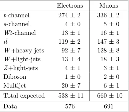
Table 1 provides the event yields for the electron and muon channels after the event
selection. The predictions are normalised to 4.6 fb−1 and their uncertainties are derived
taking into account the statistical uncertainties of the simulated samples. For the multijet background, the uncertainties on the prediction are the statistical uncertainties of the data
and simulated samples of the muon and electron channel, respectively. Figure 4shows the
angular distributions cosθ*andφ* after the event selection for the electron and muon
chan-nels in data, compared to predictions using SM couplings. The uncertainties are derived taking into account the statistical uncertainties of the data samples for data and simulated samples on the prediction and the 50% systematic uncertainty on the normalisation of the
multijet background. Since the number of events in W+light-jets and multijet samples
are low, statistical fluctuations and events with large generator weights affect the sample
shapes. Therefore, shape templates from events selected without theb-tagging requirement
are used for these two backgrounds to smooth the simulated models. In these events, the
hardest jet in the event is chosen to take the place of theb-tagged-like jet for the purposes
of the event selection and reconstruction. Overall, good agreement between the observed and expected distributions is found.
7 Analysis method
The model describing thet-channel signal in section2is connected to the angles measured
in reconstructed events via an analytic folding procedure. Models of the selection efficiency
and detector resolution are derived from simulated t-channel signal events, and a model
of the reconstructed background is derived from the sum of the combined background
processes described in section 4. Since the values of the parameters f1 and δ− depend on
top-quark couplings, both thet-channel signal and thet¯tbackground are sensitive to their
values. Only the angular distributions for the leptonic decay of theW boson are measured,
but the efficiency and resolution may also depend on other unmeasured distributions, such
as those associated with theη distribution of the top or spectator quark in the laboratory
frame. The efficiency, resolution, and background models are constructed such that they
JHEP04(2016)023
Events / 0.1
0 10 20 30 40 50 60 70 Data -channel t -channel s , Wt , t t +jets W +jets, Diboson Z Multijet MC stat. + multijet unc.
ATLAS
-1 = 7 TeV, 4.6 fb s
Electron signal region
*) θ cos(
-1 -0.8 -0.6 -0.4 -0.2 0 0.2 0.4 0.6 0.8 1
0.5 1 1.5
Data/Pred.
(a)
Events / 0.1
0 10 20 30 40 50 60 70 80 90 Data -channel t -channel s , Wt , t t +jets W +jets, Diboson Z Multijet MC stat. + multijet unc. ATLAS
-1 = 7 TeV, 4.6 fb s
Muon signal region
*)
θ
cos(
-1 -0.8 -0.6 -0.4 -0.2 0 0.2 0.4 0.6 0.8 1
0.5 1 1.5
Data/Pred.
(b)
Events / 0.1
0 10 20 30 40 50 60 70 80 90 Data -channel t -channel s , Wt , t t +jets W +jets, Diboson Z Multijet MC stat. + multijet unc.
ATLAS
-1
= 7 TeV, 4.6 fb s
Electron signal region
π */ φ
0 0.2 0.4 0.6 0.8 1 1.2 1.4 1.6 1.8 2
0.5 1 1.5
Data/Pred.
(c)
Events / 0.1
0 20 40 60 80
100 Datat-channel
-channel s , Wt , t t +jets W +jets, Diboson Z Multijet MC stat. + multijet unc.
ATLAS
-1
= 7 TeV, 4.6 fb s
Muon signal region
π
*/
φ
0 0.2 0.4 0.6 0.8 1 1.2 1.4 1.6 1.8 2
0.5 1 1.5
Data/Pred.
[image:13.595.90.512.141.558.2](d)
JHEP04(2016)023
Electrons Muons
t-channel 274±2 336±2
s-channel 4 ±0 5 ±0
Wt-channel 13 ±1 16 ±1
tt¯ 119±2 147±3
W+heavy-jets 92 ±7 128±8
W+light-jets 13 ±4 18 ±3
Z+light-jets 4 ±1 3 ±1
Diboson 1 ±0 2 ±0
Multijet 20 ±7 6 ±1
Total expected 538±11 660±10
[image:14.595.189.408.84.274.2]Data 576 691
Table 1. Event yields for the electron and muon channels in the signal region. Individual predic-tions are rounded to integers while “Total expected” corresponds to the rounding of the sum of full precision individual predictions. The uncertainties shown are statistical only. Uncertainties of less than 0.5 events appear as zero.
dependent on the values of these parameters (see appendix A). A probability density is
derived for all events in the signal region, as a function of the reconstructed angles cosθ*
and φ*, and conditional on the parameters. This density is then used to construct a
likelihood, from which f1 and δ− are measured in data.
The signal model described by Equation (2.1) is a series in spherical harmonics, only
containing terms up to a maximum value ofl,lmaxsig = 2. Describing the efficiency and
reso-lution models similarly allows the use of the orthogonality properties of spherical harmonics
to construct analytically-folded distributions [23]. An efficiency function, given by
(θ*
T, φ*T; ~α, P) = leff
max
X
l0,m0
el0,m0(α, P~ )Ym 0
l0 (θ*T, φ*T), (7.1)
describes the probability that a t-channel signal event with the given true angles θ*
T and
φ*
T will be reconstructed in the signal region. The series contains all allowed values of l
0
and m0 up to a maximum spherical harmonic degree, leff
max. The selected signal density,ρs,
is then defined as the product of the efficiency function and the signal model,ρ, normalised
to the overall rate,
ρs(θ*T, φ*T; α, P~ ) =
(θ*
T, φ*T; α, P~ )ρ(θ*T, φ*T; α, P~ ) R
(θ*
T, φ*T; ~α, P)ρ(θT*, φ*T; ~α, P)dΩ
∗
T
=X
L,M
cL,M(α, P~ )YLM(θ*T, φ*T),
for cL,M(α, P~ ) =
P
l,l0,m,m0
el0,m0(~α, P)al,m(α, P~ )Gm,m 0,M
l,l0,L
P
l,m
(−1)mel,−m(~α, P)al,m(α, P~ )
. (7.2)
The Gaunt coefficients G are defined in terms of Clebsch-Gordan coefficients Cm1m2M
JHEP04(2016)023
given by,
Gm,ml,l0,L0,M = s
(2l+ 1)(2l0+ 1)
4π(2L+ 1) C
0,0,0 l,l0,LCm,m
0,M
l,l0,L .
The efficiency function is determined from a likelihood fit to simulated t-channel events.
A value is chosen for leff
max by comparing the associated values of the corrected Akaike
Information Criteria, AICc [62,63], a likelihood-ratio test with an additional penalty term
which increases with the number of parameters. From this test, leff
max = 6 is chosen. The
deviation in the results from the selection of efficiency models with leff
max varied by±2 are
included as systematic uncertainties. Other criteria, such as the Schwarz Criteria [64],
select values of leff
max within the range chosen for this uncertainty.
When reconstructing events in the signal region, the finite resolution of the detector
results in a migration from the true angles to measured angles θ* and φ*. This migration
is modelled by the resolution function,
R(θ*, φ*|θT*, φ*T; ~α, P) =
lreco max
X
λ,µ ltrue
max
X
L0,M0
rλ,µ,L0,M0(~α, P)Yµ λ(θ
*, φ*)YM0
L0 (θ*T, φ*T). (7.3)
This series contains all terms with allowed values ofλ,µ,L0, and M0 up to the maximum
degree parametersltrue
max, associated with the dependence onθ*Tandφ*T, andlrecomax, associated
with the dependence on θ* and φ*. The reconstructed signal density, ρ
r, is defined as the
convolution of this function with the selected signal density,
ρr(θ*, φ*; ~α, P) = Z
R(θ*, φ*|θT*, φ*T; ~α, P)ρs(θ*T, φ*T; ~α, P)dΩ∗T
=X
λ,µ
dλ,µ(~α, P)Yλµ(θ∗, φ∗),
for dλ,µ(~α, P) =
X
L,M
(−1)McL,M(~α, P)rλ,µ,L,−M(~α, P). (7.4)
The resolution function is determined using a spherical Fourier technique [65]. In principle,
describing a very narrow resolution function could require large values of ltrue
max and lrecomax.
In practice, the mathematics of angular-momentum addition guarantee that there are no
terms in Equation (7.2) with L > lsigmax+leffmax. Thus, ltruemax= l
sig
max+leffmax. The parameter
lreco
max is determined using the mean integrated squared error, MISE =
R
(ρ(x)−ρˆ(x))2dx,
whereρ(x) is the true probability density and ˆρ(x) is a distribution estimating that density.
Calculating the MISE with ρr yields a broad minimum forlmaxreco >4, and for this analysis
lreco
max = 6 is chosen. The deviation in the results from the selection of resolution models
withlreco
max varied by±2 are included as systematic uncertainties.
This density of reconstructedt-channel signal events is a series in spherical harmonics,
with coefficients which are functions of the physics parameters describing the production
(P) and decay (~α) of the top quark. A background model,
β(θ*, φ*; ~α, P) =
lbkgmax
X
λ,µ
JHEP04(2016)023
is derived which is also a series in spherical harmonics, and is added to the reconstructed
signal density via the signal fraction, fs. This background function is determined from a
likelihood fit to all simulated background events in the signal region, and contains all terms
with allowed values ofλandµup to the maximum degree parameterlbkgmax. This parameter
is determined like the equivalent parameter in the efficiency function, using the AICc. The
variations in the results from the selection of background models withlbkgmax±2 are included
as systematic uncertainties.
The probability density of all events in the signal region, ρt, is the sum of the
recon-structed signal and background densities with signal fraction fs,
ρt(θ*, φ*; ~α, P, fs) = max
lreco max,l
bkg max
X
λ,µ
Aλ,µ(α, P~ )Yλµ(θ*, φ*) for
Aλ,µ(~α, P, fs) =fsdλ,µ(~α, P) + (1−fs)bλ,µ (7.6)
=fs
P
l,l0,L,m,m0,M
(−1)Me
l0,m0al,m(~α, P)Gm,m 0,M
l,l0,L rλ,µ,L,−M
P
l,m
(−1)me
l,−mal,m(α, P~ )
+ (1−fs)bλ,µ.
Figure 5 shows the data summed over the electron and muon channels for the signal
region. Three representative models are also shown: one for the SM expectations, one that
is near the expected 95% C.L. sensitivity in f1, and one near the expected sensitivity in
δ−. These values for f1 and δ− are the same as those used in figure 3, but the curves
now include the effects of efficiency, resolution and background. The main differences between the two figures are due to the isolation requirements placed on the leptons. For
cosθ*=−1, the lepton overlaps theb-tagged jet, while forφ* =π, the lepton may overlap
the spectator jet. The region where the efficiency is less than 0.05% (cosθ* <−0.95, and
−0.95<cosθ* <−0.85 forπ−0.1< φ*< π+ 0.1), is excluded from further analysis. For
other regions, the efficiency varies, as a function of φ* and cosθ*, from 0.1% up to 1.7%
for larger cosθ* and away from the plane containing the spectator jet. As the features of
the angular distributions are broad, the effects of resolution are small. The main effect is to smooth out some of the effects of the acceptance and to increase the number of events
at large cosθ* where the SM contribution is small. As seen in figure 4, the background is
also somewhat larger for large cosθ*.
An unbinned likelihood function is constructed from the probability density in
Equa-tion (7.6) and from a set of events D=
θ*
i, φ*i, wi ,i= 1,2, . . . N, L(~α) =
N Y
i=1
exp (wiρt(θi∗, φ
∗
i|~α, P, fs)), (7.7)
whereθ*
i andφ*i can be taken either from data or MC simulation, and the event weightswi
are 1 for measured data. The likelihood is evaluated on a grid with spacing 0.01 in f1 and
0.01π inδ−. The efficiency and resolution models at each point are derived fromProtos
JHEP04(2016)023
π
*/
φ
0.5 1 1.5
Events / 0.2
0 20 40 60 80 ATLAS -1
= 7 TeV, 4.6 fb s 0.5] − 1.0, − [ ∈ *) θ cos( π */ φ
0.5 1 1.5
0.5,0.0] − [ ∈ *) θ cos( π */ φ
[image:17.595.90.512.84.387.2]0.5 1 1.5
[0.0,0.5] ∈ *) θ cos( π */ φ
0.5 1 1.5
[0.5,1.0] ∈ *) θ cos( Data =0.0 (SM) − δ =0.3, 1 f π =0.1 − δ =0.3, 1 f =0.0 − δ =0.1, 1 f (a) *) θ cos( -1 -0.8 -0.6 -0.4 -0.2 0 0.2 0.4 0.6 0.8 1
Events / 0.1
0 20 40 60 80 100 Data =0.0 (SM) − δ =0.3, 1 f π =0.1 − δ =0.3, 1 f =0.0 − δ =0.1, 1 f ATLAS -1 = 7 TeV, 4.6 fb s
(b)
π
*/
φ
0 0.2 0.4 0.6 0.8 1 1.2 1.4 1.6 1.8 2
Events / 0.1
0 20 40 60 80 100 120 140 Data =0.0 (SM) − δ =0.3, 1 f π =0.1 − δ =0.3, 1 f =0.0 − δ =0.1, 1 f ATLAS -1 = 7 TeV, 4.6 fb s
(c)
Figure 5. Projections into (a)φ* in bins of cosθ*, (b) cosθ*, and (c)φ*of the function described in Equation (7.6), for different values of f1 and δ−. The black points shown are for the selected
data events with statistical uncertainties. The curves shown represent the model at the SM point f1= 0.3,δ−= 0 (solid red), and two sets of beyond-the-SM values,f1= 0.1,δ−= 0 (dashed blue)
andf1= 0.3,δ−= 0.1π(dotted green).
Interpreting these parameters as varying the coupling ratio gR/VL, the polarisation P is
varied simultaneously according to the parameterisation in ref. [24].
A central value is measured at the maximum value of L on this grid, determined from
a Gaussian fit to the points at which L is evaluated. The 68% and 95% confidence limits
are defined by the region where the likelihood ratio, L/Lmax, is larger than the value that
would yield the same likelihood for a two-dimensional Gaussian distribution. They are refined to increase the accessible precision by interpolating between points on either side of the contours determined from these evaluated points. The statistical uncertainty is estimated from the symmetrised 68% C.L. interval of each parameter.
This model is checked for closure both with MC samples, and by defining toy-MC
samples based on Equation (7.6) with the same number of events as in data. These samples
were generated at various points in (f1, δ−) space. In all cases they are found to reproduce
the expected values of f1 and δ−. These toy-MC samples were also used to derive pull
JHEP04(2016)023
8 Sources of systematic uncertaintySystematic uncertainties are evaluated in the full (f1, δ−) parameter space. Efficiency,
resolution, and background models are determined from MC samples with a parameter varied by its uncertainty, or a subset where appropriate. A likelihood is constructed from the resulting model, using events generated with nominal values of the varied parameters. The difference between the central values estimated at the nominal value of a parameter and at the value varied by its uncertainty, or half the difference between central values estimated with the parameter varied up and down by its uncertainty, is used to construct a covariance matrix for each source of systematic uncertainty. The total covariance matrix for the systematic uncertainties and its correlation matrix are found from the sum of the covariance matrices determined for individual uncertainties.
8.1 Object modelling
The uncertainties in the reconstruction of jets, leptons, and Emiss
T are propagated to the
analysis, following the same procedures as described in ref. [46]. The main source of
uncertainty from these physics objects is the jet energy scale (JES) [66], which is the
largest systematic uncertainty on the measurement of f1. To estimate the impact of the
JES uncertainty on the result, the jet energy is scaled up and down by its uncertainty [66],
which ranges from 2.5% in the central region with high-pT jets to 14% in the far forward
region with low-pT jets. Uncertainties are also estimated for jet energy resolution and
reconstruction efficiency; the impact of varying the jet-vertex fraction requirement; Emiss
T
reconstruction and the effect of pile-up collisions on the Emiss
T ; b-tagging efficiency and
mistagging rate; lepton trigger, identification, and reconstruction efficiencies; and lepton momentum, energy scale, and resolution.
8.2 MC generators and PDFs
Multiple MC event generators are used to model the t-channel and t¯t processes in this
analysis, and the differences between these generators are included as systematic
uncertain-ties. Comparing theAcerMC generator used fort-channel events and the Powheg-box
generator used for t¯t events to the Protos generator used for both the t-channel single
top-quark events and t¯t events yields the largest uncertainty in δ−. Additional t-channel
comparisons are performed between the AcerMC and Powheg-box generators and
be-tween AcerMC events with showering by Pythia and Herwig. The renormalisation
and factorisation scales in the Powheg-box t-channel sample are also varied
indepen-dently by factors of 0.5 and 2.0. Additional t¯t comparisons are performed between the
Powheg-box generator and the MC@NLO [67] generator with showering by Herwig,
and betweenPowheg-boxevents with showering byPythiaandHerwig. The variations
JHEP04(2016)023
8.3 Signal and background normalisationCross-sections for background processes given in section6are varied up and down by their
uncertainties. The multijet normalisation is varied by 50% as discussed in section 6, and
the remaining backgrounds are varied simultaneously to produce a conservative estimate.
The impact of object modelling and other uncertainties on the W+jets background
nor-malisation are considered in parallel with the variations made in t-channel andt¯tsamples.
A separate shape uncertainty is assigned to the W+jets samples by varying the matching
and factorisation scales in the Alpgen generator. The integrated luminosity is varied up
and down by its uncertainty, ±1.8%, derived as detailed in ref. [29].
8.4 Detector correction and background parameterisation
An uncertainty due to the limited size of the MC samples used to estimate the efficiency and resolution models is estimated from the statistical uncertainties derived from a
mea-surement off1andδ−in thet-channel signal MC sample alone. The background statistical
uncertainty is estimated by varying the background model according to the eigenvectors of its covariance matrix. The background statistical uncertainty dominates the total “MC
statistics” uncertainty listed in table 2. Its significance reflects the small size of some
background samples in the signal region, and the resulting disparate values of the sample
weights. The effect of varying the cutoff degree lmax in the determination of these models
is also estimated, and is found to be small compared to MC statistical uncertainty.
8.5 Uncertainty combination
Table 2 shows the contribution of each source of uncertainty to the measurement of the
parametersf1 andδ−and their correlation,ρ(f1, δ−). The total systematic uncertainty and
correlation is obtained from the sum of the covariance matrices determined for each source. It is combined with the covariance matrix of the statistical uncertainty via the following
method. At each point ~αi in the (f1, δ−) space, a multivariate normal distribution Ni is
constructed with the covariance matrix representing the systematic uncertainties, Σsyst,
and the mean, ~αi. The resulting distribution is evaluated at a point α~j and multiplied by
the likelihood at this point,Lstat
j . The maximum modified likelihood value, over all possible
pointsα~j, is kept, and the resulting broadened likelihood distribution Lstat+systi is used to
represent the measurement with both statistical and systematic variation incorporated:
Lstat+systi = maxj
Ni(α~j;α~i,Σsyst)· Lstatj . (8.1)
The resulting confidence limits are taken as the full uncertainty in the measurement.
9 Results
The result for (f1, δ−) and the coupling ratios (Re [gR/VL],Im [gR/VL]) is shown in figure6.
The 68% contour represents the total uncertainty on the measurement.
The parameters f1 and δ− and their uncertainties are measured to be
f1 = 0.37±0.05 (stat.)±0.05 (syst.),
δ− =−0.014π±0.023π (stat.)±0.028π (syst.).
JHEP04(2016)023
Source σ(f1) σ(δ−)/π ρ(f1, δ−)
Data statistics 0.05 0.023 0.01
Jets 0.03 0.015 0.39
b-tagging <0.01 <0.001 −0.70
Leptons 0.02 0.007 0.39
Emiss
T 0.01 0.004 −0.27
Generator 0.02 0.017 0.40
Parton shower 0.02 0.001 0.98
PDF variations 0.01 0.009 0.23
Cross-sections <0.01 <0.001 1.00
W+jets shape <0.01 0.001 −0.59
Multijet normalisation <0.01 0.002 −1.00
Luminosity <0.01 <0.001 −1.00
Modellmax variation 0.01 0.001 −0.70
MC statistics 0.02 0.011 0.14
Combined systematic 0.05 0.028 0.27
[image:20.595.163.430.83.364.2]Total 0.07 0.036 0.15
Table 2. Sources of systematic uncertainty on the measurement off1 andδ− using AcerMC t -channel single top-quark simulated events and backgrounds estimated from both MC simulation and data, including Powheg-box t¯t simulation. Individual sources are evaluated separately for shifts up and down, and symmetrised uncertainties σ(f1), σ(δ−) and correlation coefficients ρ(f1, δ−)
are given.
The correlation in the measurement of these parameters is ρ(f1, δ−) = 0.15. The results
are compatible with the SM expectations at LO, derived from expressions in refs. [11,68]
withmt= 172.5 GeV, mW = 80.399 GeV, and mb = 4.95 GeV: f1= 0.304 and δ−= 0.
The dependence of the parameters f1 andδ− on the top-quark mass is evaluated using
t-channel and t¯t simulation samples with a range of different top-quark masses. A linear
dependence is found, resulting from changes in acceptance at different masses, with a slope
of −0.019 GeV−1 for f
1 and a negligible slope for δ−. The uncertainty due to the
top-quark mass dependence is not included in the total systematic uncertainty since it has no significant impact on the results.
The propagation of the uncertainties to the (Re [gR/VL],Im [gR/VL]) space gives
Re
gR VL
=−0.13 ±0.07 (stat.)±0.10 (syst.),
Im
gR VL
= 0.03 ±0.06 (stat.)±0.07 (syst.).
(9.2)
The correlation in the measurement of these coupling ratios is
JHEP04(2016)023
1 f
0.1 0.2 0.3 0.4 0.5 0.6
Likelihood (Arb. Units)
0 0.2 0.4 0.6 0.8 1 1.2 1.4 ATLAS -1 = 7 TeV, 4.6 fb s Likelihood Best Fit SM Gaussian fit σ 1 σ 2 (a) − δ
-0.15 -0.1 -0.05 0 0.05 0.1 0.15
Likelihood (Arb. Units)
0 0.2 0.4 0.6 0.8 1 1.2 1.4 ATLAS -1
= 7 TeV, 4.6 fb s Likelihood Best Fit SM Gaussian fit σ 1 σ 2 (b) − δ
-0.15 -0.1 -0.05 0 0.05 0.1 0.15
1 f 0.1 0.2 0.3 0.4 0.5
0.6 ATLAS -1 = 7TeV, 4.6 fb s Best Fit SM 68% CL 95% CL (c) ] L /V R Im[g -0.4 -0.3 -0.2 -0.1 0 0.1 0.2 0.3 0.4
]L /V R Re[g -0.6 -0.4 -0.2 0 0.2 0.4 ATLAS -1
[image:21.595.93.508.96.432.2]= 7TeV, 4.6 fb s Best Fit SM 68% CL 95% CL (d)
Figure 6. Projections of the likelihood function constructed from the signal region probability density Equation (7.6) and data events into (a) f1, (b) δ−, (c) f1 vs. δ−, and (d) Re [gR/VL] vs. Im [gR/VL], with systematic uncertainties incorporated. The black points indicate the largest evaluated likelihood in each bin of the projected variable. Gaussian fits to the one-dimensional projections were performed, displayed as the red curve. Regions shown in green and yellow represent the 68% and 95% confidence level regions, respectively. A black line or cross indicates the observed value, and the grey line or point indicates the SM expectation.
uncertainty in the top-quark, W boson and b-quark masses [69] is < 0.01 in Re [gR/VL],
and <0.0001 in Im [gR/VL].
Limits are placed simultaneously on the possible complex values of the ratio of the
anomalous couplings gR and VL at 95% C.L.,
Re
gR VL
∈[−0.36,0.10] and Im
gR VL
∈[−0.17,0.23]. (9.3)
The best constraints on Re [gR] come from W boson helicity fractions in top-quark
decays, with Re [gR] of [−0.08,0.04] and [−0.08,0.07], both at 95% C.L., from ATLAS [17]
and from CMS [18], respectively. However, these limits use the measured single top-quark
production cross-section [46,70] along with the assumption that VL = 1 and Im [gR] = 0.
JHEP04(2016)023
excluded. The limits presented in this paper remove these assumptions and extend the
knowledge of gR to the whole complex plane by simultaneously measuring information
about Re [gR/VL] and Im [gR/VL]; the latter is previously unmeasured.
10 Conclusion
The analysis described in this publication is a two-dimensional measurement of anomalous
couplings in the Wtb vertex in t-channel single top-quarks events, performed on 4.6 fb−1
of pp collisions at a centre-of-mass energy of 7 TeV collected by the ATLAS detector at
the LHC. An analytic folding model and likelihood maximisation techniques are used to
extract values of the parameters f1 and δ− in a parameterisation of the decay of the
top quark, which translate to limits on the couplings Re [gR/VL] and Im [gR/VL] with
VR = gL = 0. The coupling parameterisation in terms of the spherical angles θ* and
φ* defines the angular distribution of the t-channel signal process. Efficiency and
resolu-tion funcresolu-tions are fit in this space, which are then folded into the signal model describing the underlying physics analytically. A background function is fit and added to the signal model. The full model is used to construct a likelihood and its characterisation provides
es-timators of the best-fit central value, uncertainties, and correlations betweenf1 and δ−, or
Re [gR/VL] and Im [gR/VL]. The result is combined with estimated sources of systematic
un-certainty to give the measurement of the parameters, f1= 0.37±0.05 (stat.)±0.05 (syst.),
δ− = −0.014π±0.023π (stat.)±0.028π (syst.), and ρ(f1, δ−) = 0.15, or Re [gR/VL] =
−0.13 ±0.07 (stat.)±0.10 (syst.), Im [gR/VL] = 0.03 ±0.06 (stat.)±0.07 (syst.), and
ρ(Re [gR/VL],Im [gR/VL]) = 0.11 in terms of the couplings. The measurement sets limits
at the 95% confidence level on Re [gR/VL]∈ [−0.36,0.10] and Im [gR/VL]∈ [−0.17,0.23].
The limits on Re [gR/VL] are complementary to limits from B-meson decay and W
helic-ity measurements, and contain previously unmeasured information about Im [gR/VL]. The
measured values are in agreement with SM expectations.
Acknowledgments
We thank CERN for the very successful operation of the LHC, as well as the support staff from our institutions without whom ATLAS could not be operated efficiently.
We acknowledge the support of ANPCyT, Argentina; YerPhI, Armenia; ARC, Aus-tralia; BMWFW and FWF, Austria; ANAS, Azerbaijan; SSTC, Belarus; CNPq and FAPESP, Brazil; NSERC, NRC and CFI, Canada; CERN; CONICYT, Chile; CAS, MOST and NSFC, China; COLCIENCIAS, Colombia; MSMT CR, MPO CR and VSC CR, Czech Republic; DNRF, DNSRC and Lundbeck Foundation, Denmark; IN2P3-CNRS, CEA-DSM/IRFU, France; GNSF, Georgia; BMBF, HGF, and MPG, Germany; GSRT, Greece; RGC, Hong Kong SAR, China; ISF, I-CORE and Benoziyo Center, Israel; INFN, Italy; MEXT and JSPS, Japan; CNRST, Morocco; FOM and NWO, Netherlands; RCN, Nor-way; MNiSW and NCN, Poland; FCT, Portugal; MNE/IFA, Romania; MES of Russia and
NRC KI, Russian Federation; JINR; MESTD, Serbia; MSSR, Slovakia; ARRS and MIZˇS,
JHEP04(2016)023
JHEP04(2016)023
A Parameter dependence of the folding and background modelsThe derivation of the efficiency, resolution, and background models, described in
Equa-tions (7.1)–(7.6), is based on the form of these distributions in MC simulation. For the
background model, constructed from the sum of all predicted backgrounds with an ap-preciable effect on the distribution, this includes events containing top quarks, primarily
fromt¯tproduction, the distribution of which is affected by changing the values of the
cou-plings VL and gR. The efficiency and resolution models are averages over all unmeasured
distributions in the signal. Variations in the values of VL and gR alter those unmeasured
distributions, which could lead to a dependence on these couplings for the efficiency and
resolution models. For instance,t-channel single top-quark production depends on
anoma-lous coupling in both the top-quark production and decay vertices, so varying the couplings
alters production-side distributions, such as the pT andη distributions of the top or
spec-tator quark.
To test how these potential sources of dependence affect the models, closure tests are
performed with input MC events generated at different values of the parameters f1 and
δ− using efficiency, resolution, and background models derived from MC events generated
with SM parameter values. The t-channel signal and t¯t background events are generated
with Protos for both the input MC events and the events used to derive the models.
The results of these closure tests can then be compared to the values with which the input events were generated; any trend connecting them other than a line with a slope of one and an intercept of zero indicates a dependence which could bias the measurement. The
results of these tests, shown in figure 7, indicate biases in the extracted parameters.
If the biases shown are due to the mismatch between the values of f1 and δ− in the
efficiency, resolution, and background models, they can be removed by varying these pa-rameters in the functions describing these models to match their values in the signal model.
This is achieved by deriving these models from t-channel signal MC events representing
each point in (f1, δ−) independently, and calculating the likelihood using the same f1 and
δ− in the signal model and in the t-channel signal MC events. The results of these tests,
shown in figure 8, indicate that this procedure eliminates the biases shown in figure 7.
JHEP04(2016)023
(gen)
1
f
0.1 0.2 0.3 0.4 0.5
(fit)1 f 0.05 0.1 0.15 0.2 0.25 0.3 0.35 0.4 0.45 Simulation ATLAS -1
= 7 TeV, 4.6 fb s 1 Extracted f Quadratic fit (a) (gen) − δ 0.15
− −0.1 −0.05 0 0.05 0.1 0.15 0.2
(fit)− δ 0.2 − 0.1 − 0 0.1 0.2 0.3 Simulation ATLAS -1
[image:25.595.93.504.111.280.2]= 7 TeV, 4.6 fb s − δ Extracted Linear fit (b)
Figure 7. Biases in the estimation of the values of the parameters (a) f1 and (b) δ− which arise when the efficiency, resolution, and background models are determined from SM simulated events, wheref1= 0.3 andδ− = 0. The points represent the central values obtained from the likelihood fit,
with the expected statistical uncertainty in 4.6 fb−1of data at√s= 7 TeV shown by the error bars. The dashed line with a slope of one and intercept of zero, representing no bias in the measurement, is added to guide the eye. A non-negligible bias is evident, and is represented at the lowest reasonable order with a polynomial fit. For δ− a linear fit is sufficient, while for f1 a quadratic fit gives a better description.
(gen)
1
f
0.1 0.2 0.3 0.4 0.5
(fit)1 f 0.1 0.2 0.3 0.4
0.5 ATLASs = 7 TeV, 4.6 fb Simulation-1
1 Extracted f Linear fit (a) (gen) − δ 0.15
− −0.1 −0.05 0 0.05 0.1 0.15 0.2
(fit)− δ 0.2 − 0.15 − 0.1 − 0.05 − 0 0.05 0.1 0.15 0.2 Simulation ATLAS -1 = 7 TeV, 4.6 fb s − δ Extracted Linear fit (b)
Figure 8. Comparison of the estimation of the values of the parameters (a)f1and (b)δ−derived by
[image:25.595.95.507.439.608.2]JHEP04(2016)023
Open Access. This article is distributed under the terms of the Creative CommonsAttribution License (CC-BY 4.0), which permits any use, distribution and reproduction in
any medium, provided the original author(s) and source are credited.
References
[1] CDFcollaboration, F. Abe et al., Observation of top quark production inpp¯ collisions,Phys. Rev. Lett.74 (1995) 2626[hep-ex/9503002] [INSPIRE].
[2] D0collaboration, S. Abachi et al.,Observation of the top quark,Phys. Rev. Lett.74(1995) 2632[hep-ex/9503003] [INSPIRE].
[3] CDFcollaboration, T. Aaltonen et al.,First Observation of Electroweak Single Top Quark
Production,Phys. Rev. Lett.103(2009) 092002[arXiv:0903.0885] [INSPIRE].
[4] D0collaboration, V.M. Abazov et al., Observation of Single Top Quark Production,Phys. Rev. Lett.103(2009) 092001 [arXiv:0903.0850] [INSPIRE].
[5] A.D. Martin, W.J. Stirling, R.S. Thorne and G. Watt,Parton distributions for the LHC, Eur. Phys. J.C 63(2009) 189[arXiv:0901.0002] [INSPIRE].
[6] N. Kidonakis,Next-to-next-to-leading-order collinear and soft gluon corrections for t-channel single top quark production, Phys. Rev.D 83(2011) 091503[arXiv:1103.2792] [INSPIRE].
[7] J.A. Aguilar-Saavedra,A minimal set of top anomalous couplings, Nucl. Phys.B 812(2009) 181[arXiv:0811.3842] [INSPIRE].
[8] J.A. Aguilar-Saavedra,A minimal set of top-Higgs anomalous couplings, Nucl. Phys.B 821
(2009) 215[arXiv:0904.2387] [INSPIRE].
[9] K.G. Wilson,Nonlagrangian models of current algebra,Phys. Rev.179(1969) 1499
[INSPIRE].
[10] W. Buchm¨uller and D. Wyler,Effective Lagrangian Analysis of New Interactions and Flavor Conservation,Nucl. Phys.B 268(1986) 621[INSPIRE].
[11] J.A. Aguilar-Saavedra and J. Bernabeu, W polarisation beyond helicity fractions in top quark decays,Nucl. Phys.B 840(2010) 349[arXiv:1005.5382] [INSPIRE].
[12] B. Grzadkowski and M. Misiak, Anomalous Wtb coupling effects in the weak radiative B-meson decay,Phys. Rev. D 78(2008) 077501[Erratum ibid. D 84(2011) 059903] [arXiv:0802.1413] [INSPIRE].
[13] Q.-H. Cao, B. Yan, J.-H. Yu and C. Zhang,A general analysis of W tbanomalous couplings,
arXiv:1504.03785[INSPIRE].
[14] W. Bernreuther, P. Gonzalez and M. Wiebusch,The Top Quark Decay Vertex in Standard Model Extensions,Eur. Phys. J.C 60(2009) 197[arXiv:0812.1643] [INSPIRE].
[15] L. Duarte, G.A. Gonz´alez-Sprinberg and J. Vidal,Top quark anomalous tensor couplings in the two-Higgs-doublet models,JHEP 11(2013) 114[arXiv:1308.3652] [INSPIRE].
[16] CDFandD0collaborations, T. Aaltonen et al.,Combination of CDF and D0 measurements
of theW boson helicity in top quark decays,Phys. Rev.D 85(2012) 071106
[arXiv:1202.5272] [INSPIRE].
JHEP04(2016)023
[18] CMScollaboration, Measurement of the W-boson helicity in top-quark decays fromt¯t
production in lepton+jets events in pp collisions at√s= 7TeV,JHEP 10(2013) 167
[arXiv:1308.3879] [INSPIRE].
[19] CMScollaboration, Measurement of the W boson helicity in events with a single
reconstructed top quark in pp collisions at√s= 8TeV,JHEP 01(2015) 053
[arXiv:1410.1154] [INSPIRE].
[20] G. Mahlon and S.J. Parke, Improved spin basis for angular correlation studies in single top quark production at the Tevatron,Phys. Rev. D 55(1997) 7249[hep-ph/9611367] [INSPIRE].
[21] G. Mahlon and S.J. Parke, Single top quark production at the LHC: Understanding spin, Phys. Lett.B 476(2000) 323[hep-ph/9912458] [INSPIRE].
[22] R. Schwienhorst, C.P. Yuan, C. Mueller and Q.-H. Cao,Single top quark production and decay in thet-channel at next-to-leading order at the LHC,Phys. Rev.D 83(2011) 034019
[arXiv:1012.5132] [INSPIRE].
[23] J. Boudreau, C. Escobar, J. Mueller, K. Sapp and J. Su,Single top quark differential decay rate formulae including detector effects,arXiv:1304.5639[INSPIRE].
[24] J.A. Aguilar-Saavedra and S.A. dos Santos,New directions for top quark polarization in the t-channel process,Phys. Rev.D 89(2014) 114009 [arXiv:1404.1585] [INSPIRE].
[25] J.A. Aguilar-Saavedra,Single top quark production at LHC with anomalous Wtb couplings, Nucl. Phys.B 804(2008) 160[arXiv:0803.3810] [INSPIRE].
[26] ATLAScollaboration,The ATLAS Experiment at the CERN Large Hadron Collider,2008 JINST 3S08003[INSPIRE].
[27] ATLAScollaboration,Performance of the ATLAS Trigger System in 2010, Eur. Phys. J.C
72(2012) 1849[arXiv:1110.1530] [INSPIRE].
[28] L. Evans and P. Bryant,LHC Machine,2008JINST 3S08001[INSPIRE].
[29] ATLAScollaboration,Improved luminosity determination in pp collisions at √s= 7TeV using the ATLAS detector at the LHC,Eur. Phys. J.C 73 (2013) 2518[arXiv:1302.4393] [INSPIRE].
[30] ATLAScollaboration,Performance of the ATLAS muon trigger in pp collisions at √s= 8TeV,Eur. Phys. J.C 75(2015) 120[
arXiv:1408.3179] [INSPIRE].
[31] B.P. Kersevan and E. Richter-Was,The Monte Carlo event generator AcerMC versions 2.0
to 3.8 with interfaces to PYTHIA 6.4, HERWIG 6.5 and ARIADNE 4.1,Comput. Phys.
Commun.184(2013) 919[hep-ph/0405247] [INSPIRE].
[32] J. Pumplin, D.R. Stump, J. Huston, H.L. Lai, P.M. Nadolsky and W.K. Tung, New generation of parton distributions with uncertainties from global QCD analysis,JHEP 07
(2002) 012[hep-ph/0201195] [INSPIRE].
[33] B.P. Kersevan and I. Hinchliffe,A consistent prescription for the production involving massive quarks in hadron collisions,JHEP 09(2006) 033[hep-ph/0603068] [INSPIRE].
[34] T. Sj¨ostrand, S. Mrenna and P.Z. Skands,PYTHIA 6.4 Physics and Manual,JHEP 05
(2006) 026[hep-ph/0603175] [INSPIRE].


![Figure 6.Projections of the likelihood function constructed from the signal region probabilitydensity Equation (7.6) and data events into (a) f1, (b) δ−, (c) f1 vs.δ−, and (d) Re [gR/VL]vs](https://thumb-us.123doks.com/thumbv2/123dok_us/7803207.170794/21.595.93.508.96.432/figure-projections-likelihood-function-constructed-signal-probabilitydensity-equation.webp)

