DEVELOPMENT OF STATISTICAL AND
GEOSPATIAL-BASED FRAMEWORK FOR
DROUGHT-RISK ASSESSMENT
A Thesis submitted by
Kavina Shaanu Dayal
BSc (Meteorology)
MSc (Meteorology)
For the award of
Doctor of Philosophy
Drought is an insidious, complex and one of the least understood natural phenomena resulting from a deficiency of water resources. While droughts cannot be prevented, its impacts, however, can be mitigated through proper design of water storage infrastructure and management strategies. A comprehensive drought management plan necessitates the development of a framework that can help reduce the drought-related risk. In Australia, there are limited drought vulnerability and risk assessment models that must (1) include the drought monitoring index that measures the supply-demand balance of water resources, (2) incorporate large-scale climate drivers influencin g amplitude of drought events in the statistical prediction models, and (3) objectively quantify the drought-risk on both temporal and spatial scales. The goal of this study is to apply statistical and geospatial tools in developing a framework for assessing drought-related risks in light of improving the drought mitigation strategies.
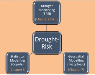
A new, temporal and spatial-explicit analytical framework for drought-risk assessment is developed based on three objectives focussed in the drought-prone southeast Queensland (SEQ) region. (1) Evaluating and affirming the suitability of the Standardised Precipitation-Evapotranspiration Index (SPEI) for the characterisation of drought events. (2) Developing a copula-based statistical, probabilistic model for predicting the SPEI and the jointly distributed drought properties (i.e., durations, severities and intensities) conditional on the large-scale climate mode indices. (3) Developing a spatially descriptive drought-risk index by combining the drought hazard, exposure and vulnerability factors using a fuzzy logic algorithm.
Southern Oscillation indicators). The vine copula algorithm is employed to derive the bivariate and trivariate joint-distributions of drought variables for conditiona l probability-based predictions. The results yield marginal differences between the observed and the predicted drought properties, elucidating the effectiveness of copula functions in drought-risk modelling. The results have implications for drought and aridity management in agricultural regions where complex relationships between climate drivers and drought properties are likely to exacerbate the risk of a future event. The third objective develops a methodology using vulnerability, exposure and hazard indicators to provide a spatio-temporal framework for drought-risk assessment. The conditional joint probability of each drought indicator is estimated using the Bayes theorem. Various fuzzy membership functions are then applied to standardise and aggregate the indicators to derive drought vulnerability, exposure and hazard indices . The resulting indices are integrated with fuzzy GAMMA overlay operation to generate optimal drought-risk maps. The maps reveal varying levels of drought risk in different austral seasons and annually that is well represented by the drought hazard index, i.e.,
This thesis is entirely the work of Kavina Shaanu Dayal except where otherwise acknowledged. The work is original and has not previously been submitted for any other award, except where acknowledged.
Principal Supervisor: Dr Ravinesh C. Deo
Associate Supervisor: Professor Armando A. Apan
Refereed Journal Articles
1. Dayal Kavina S., R. C. Deo and A. A. Apan, (2018) “Investigating drought duration-severity-intensity characteristics using Standardised Precipitation-Evapotranspiration Index: a case study in drought-prone, southeast Queensland”, ASCE Journal of Hydrologic Engineering, 23(1), 1-16. (Impact Factor = 1.600, Quartile 1 in Civil & Structural Engineering).
2. Dayal Kavina S., R. C. Deo and A. A. Apan, (2018) “Spatio-temporal
drought-risk mapping approach for southeast Queensland, Australia”, Natural Hazards, (Accepted). (Impact Factor = 1.776, Quartile 1 in Water Science and Technology).
3. Dayal Kavina S., R. C. Deo and A. A. Apan, (2018) “Development of a copula-statistical drought prediction model using the Standardised Precipitation-Evapotranspiration Index”, Water Resources Planning and Management, (In preparation). (Impact Factor = 3.05, Quartile 1 in Civil & Structural Engineering).
4. Dayal Kavina S., R. C. Deo and A. A. Apan, (2018) “Trend analysis of drought events based on SPEI: a case study”, Atmospheric Research, (In Preparation). (Impact Factor = 3.778, Quartile 1 in Atmospheric Science).
Refereed Conference Proceedings/Book Chapters
1. Dayal, Kavina S, Deo Ravinesh C, Apan Armando A, (2017) Drought
Modelling Based on Artificial Intelligence and Neural Network Algorithms: A Case Study in Queensland, Australia. In Leal Filho, W. (Ed) Climate Change Adaptation in Pacific Countries: Fostering Resilience and Improving the Quality of Life. Springer, Berlin. ISBN 978-3-319-50093-5. DOI: 10.1007/978-3-319-50094-2_11. Page 177-198.
(https://link.springer.com/chapter/10.1007%2F978-3-319-50094-2_11).
2. Dayal, Kavina S. and Deo, Ravinesh C. and Apan, Armando
A, (2016) Application of hybrid artificial neural network algorithm for the prediction of Standardised Precipitation Index. In: 2016 IEEE Region 10 International Conference: Technologies for Smart Nation (TENCON 2016), 22-25 Nov 2016, Singapore.
Foremost, I would like to express my sincere appreciation to my Principal Supervisor, Dr Ravinesh Deo for the project idea, his wisdom, direction and motivation all throughout this research journey.
The guidance and involvement of my Associate Supervisor, Professor Armando Apan, significantly helped me in framing up this thesis right from the very beginning.
My sincere gratitude also goes to University of Southern Queensland (USQ) Office of Research and Graduate Studies for the USQ Postgraduate Research Scholarship and the School of Agricultural, Computational and Environmental Sciences for providing financial support through casual teaching contracts.
This thesis would neither be accomplished nor completed without free access to datasets. As such, my heartfelt appreciation goes to the Australian Water Availability Project (AWAP), Scientific Information for Land Owners (SILO), Australian Bureau of Statistics (ABS), Queensland Government – Queensland Spatial Catalogue (QSpatial), Australian Bureau of Meteorology (BoM), Climate Prediction Centre (CPC) and the Terrestrial Ecosystem Research Network (TERN) from where the data have been sourced.
I would also like to thank Dr Doo-Woo Kim (Seoul Korea), Wen Yang, Dr Rodolfo Espada (USQ) and Peter Brigg (AWAP - CSIRO) for their prompt response to my queries. I thank my research group members and friends for providing their support and motivation.
Application of Statistical and Geospatial Tools for Drought-Risk
Assessment i
Abstract ii
Certification of Thesis iv
Publications v
Acknowledgments vi
Table of Contents vii
List of Figures x
List of Tables xiii
Acronyms and Abbreviations xv
Chapter 1 1
Introduction 1
1.1 Background 1
1.2 Statement of the Problem 4
1.3 Research Aims and Objectives 7
1.4 Significance of the Study 9
1.5 Organisation of the Thesis 10
Chapter 2 11
Literature Review 11
2.1 Bureau of Meteorology definitions of drought 11
2.2 Drought Monitoring 13
2.2.1 Existing indices for drought monitoring 14
2.2.2 Selection of indicators and indices 21
2.2.3 Comparison of existing drought indices for quantifying drought events 21 2.2.4 Standardised Precipitation-Evapotranspiration Index (SPEI) for drought
monitoring 27
2.3 Drought Modelling 29
2.3.1 Drought forecasts and predictions 30
2.3.2 Univariate drought modelling 34
2.3.3 Use of copula in hydrology 34
2.3.4 Role of climate mode indices on droughts 37
2.3.5 Copula-based drought analysis using climate mode indices 38
2.4 Geospatial Representation of Drought-risk 39
2.4.1 Vulnerability assessment 40
2.4.2 Drought vulnerability assessment 41
2.4.3 GIS-based integrated fuzzy logic 47
2.5 Summary of Chapter 48
Chapter 3 50
Data and Study Area 50
3.2.2 Data pre-processing 59
3.2.3 Data limitations 59
3.3 Location of the Study Area 60
3.4 Scope and Limitation of the Study 63
3.5 General Methodology 64
3.6 Summary of Chapter 65
Chapter 4 66
Drought indices comparison and trend analysis 66
4.1 Introduction 66
4.2 Materials and Method 68
4.2.1 Hydrological data and study area 68
4.2.2 Theoretical overview 70
4.2.2.1 Standardised Precipitation-Evapotranspiration Index (SPEI) 70 4.2.2.2 Rainfall Decile-based Drought Index (RDDI) 71 4.2.2.3 Standardised Precipitation Index (SPI) 71
4.2.2.4 Rainfall Anomaly Index (RAI) 73
4.2.2.5 Wavelet Analysis (WA) 73
4.2.2.6 Change-Point Analysis (CPA) 74
4.3 Results and Discussion 76
4.3.1 Comparison between DIs 76
4.3.2 Trend changes in the SPEI 82
4.4 Conclusion 86
Chapter 5 87
Investigating drought duration-severity-intensity characteristics using the Standardised Precipitation-Evapotranspiration Index 87
5.1 Introduction 87
5.2 Materials and Method 88
5.2.1 Hydrological data and study area 88
5.2.2 Characterisation of drought properties 91
5.3 Results and Discussion 94
5.4 Conclusions 119
Chapter 6 121
Development of copula-statistical drought prediction model using the Standardised Precipitation-Evapotranspiration Index 121
6.1 Introduction 121
6.2 Materials and Methods 123
6.2.1 Theoretical background 123
6.2.1.1 Copula Theory 123
6.2.1.3 Vine Copula 125
6.2.1.4 Conditional Prediction Model 127
6.2.1.5 Joint Return Periods 127
6.2.2 Study area and data 129
6.2.2.1 Characterisation of Drought Properties 130 6.2.2.2 Copula-Statistical Model Development 130 6.2.2.3 Selection of Marginal Distributions 132
6.3.1 Applications on SPEI and climate mode indices 140 6.3.2 Applications on drought properties and climate mode indices 149
6.3.3 Applications on drought properties 156
6.4 Further Discussion 158
6.5 Conclusion 161
Chapter 7 163
Spatio-temporal drought-risk mapping approach for southeast
Queensland, Australia 163
7.1 Introduction 163
7.2 Theoretical Overviews 165
7.2.1 Concept of vulnerability, exposure and risk 165
7.2.2 Fuzzy logic approach 166
7.3 Materials and Method 168
7.3.1 Identification and significance of factors 169
7.3.2 Study area 174
7.3.3 Proposed weighting scheme 174
7.3.4 Bayesian joint conditional probability 178
7.3.5 Framework for derivation of drought-risk map 179
7.3.6 Validation of the drought-risk index 185
7.4 Results and Discussion 186
7.5 Conclusions 197
Chapter 8 198
Conclusion 198
8.1 Introduction 198
8.2 Summary of Findings 198
8.3 Recommendations for Future Works 202
References 204
Figure 1.1: Three main objectives of this study. ...8 Figure 2.1: Rainfall deciles for the period 1 November 2001 to 31 October 2009 [Source: Australian Bureau of Meteorology]... 12 Figure 3.1: Map of the study region. Colour shading depicts digital elevation model (DEM) (meters). MDB refers to the Murray Darling Basin. ... 62 Figure 3.2: Flowchart describing general methodology of the study. ... 64 Figure 4.1: Map of point-based study locations: R1 – Subtropical, R2 – Grassland, R3 – Temperate, and R4 – Desert. ... 69 Figure 4.2: Area plot of the monthly SPEI from 1915 to 2016 for (a) R1, (b) R2, (c) R3 and (d) R4. ... 77 Figure 4.3: Area plot of the monthly SPI from 1915 to 2016 for (a) R1, (b) R2, (c) R3 and (d) R4. ... 77 Figure 4.4: Continuous wavelet transform (CWT) power spectrum for the time series of upper layer soil moisture (WRel1), SPEI, SPI, RDDI and RAI drought indices. .. 79 Figure 4.5: Cross-wavelet spectrum (XWT) between the upper layer soil moisture
(WRel1) and drought indices. ... 81 Figure 4.6: CUSUM chart of the SPEI data for location R2 with significant changes shown in the background. ... 83 Figure 4.7: CUSUM chart of the SPEI data for location R3 with significant changes shown in the background. ... 84 Figure 4.8: CUSUM chart of SPEI data for location R4 with significant changes shown in the background. ... 86 Figure 5.1: Monthly climatology of (a) precipitation (P; mm), (b) maximum
temperature (Tmax; ˚C), (c) climatic water balance (mm), and (d) upper layer soil
moisture (WRel1; fractional). Legend applies to all panels... 89 Figure 5.2: Violin plots with a combination of boxplot and kernel density distribution for (a, b) precipitation (P), (c, d) maximum temperature (Tmax), and (e, f) upper layer soil moisture (WRel1) on 3-month and 12-month timescales. ... 90 Figure 5.3: Graphical definition of drought onset and termination, drought severity
... 98 Figure 5.6: Cross-correlation of SPEI with precipitation (P) (a, f, k, and p), upper layer soil moisture (WRel1) (b, g, l, and q), upper layer end of month soil moisture
(WRel1End) (c, h, m, and r), maximum temperature (Tmax) (d, i, n, and s), and reference evapotranspiration (ETo) (e, j, o, and t). Solid lines indicate 95%
confidence interval. ... 100 Figure 5.7: Annually accumulated drought duration (D), severity (S) and intensity (I) for: (a) R1, (b) R2, (c) R3 and (d) R4 at 3-, 6-, 9-, and 12-month timescales,
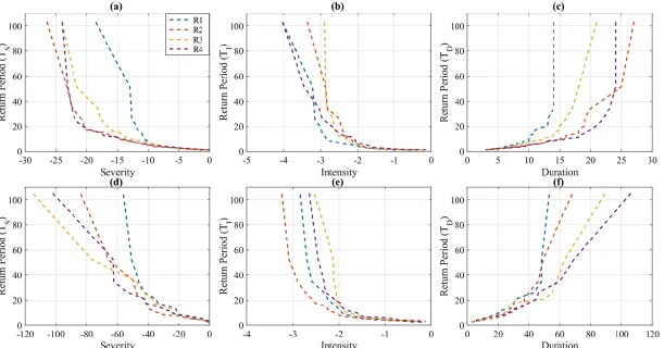
respectively. Legend applies to all panels. ... 102 Figure 5.8: The drought return period based on severity (a, d), intensity (b, e) and duration (c, f) for 3-month (row 1) and 12-month (row 2) timescales. Legend applies to all panels. ... 105 Figure 5.9: SPEI and precipitation (P) for different timescales taken for part of the Millennium Drought (2004-2010), for (a) 3, (b) 6, (c) 9, and (d) 12-month
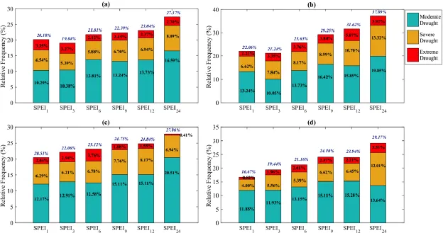
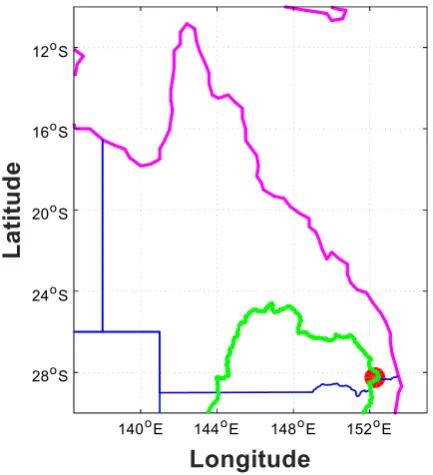
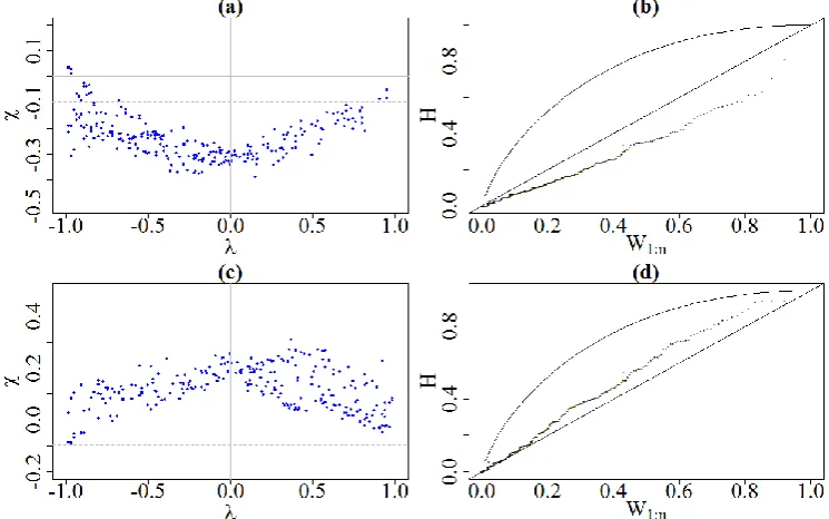
timescales, for locations R1, R2, R3 and R4, respectively. Legend applies to all panels... 111 Figure 5.10: Drought class relative frequency for SPEI timescales (1, 3, 6, 9, 12, and 24 months) for (a) R1, (b) R2, (c) R3 and (d) R4. Legend applies to all panels. ... 113 Figure 5.11: Taylor diagram displaying comparison with monthly observation (SPEI – red) with precipitation (P), reference evapotranspiration (ETo), soil moisture (WRel1 and WRel1End), and maximum temperature (Tmax) for different timescales taken at location R1. ... 118 Figure 6.1: Map of the study location R3. ... 129 Figure 6.2: Chi-plots with “confidence band at = 0.1 (dashed lines) for SPEI with (a) Niño 4 SST and (c) SOI. K-plots with the straight line (y = x) and a smooth curve
for (b) Niño 4 SST and (d) SOI joint distribution. ... 141 Figure 6.3: Observed vs. 2,000 random simulated SPEI samples (a, b). Scatter plot of observed versus predicted SPEI given information of Niño 4 SST and EMI using bivariate (c) Frank (for Niño 4 SST; red) and Gumbel (for SOI; blue) copula and using trivariate (d) Frank copula given combined information of Niño SST and SOI. ... 143 Figure 6.4: Conditional probability distribution of SPEI given SOI and Niño 4 SST values using bivariate Gumbel (a) and Frank (b) copula. The Niño 4 SST’ is in degrees Celsius. ... 147 Figure 6.5: Conditional probability distribution of SPEI different Niño 4 SST (˚C) and SOI values using trivariate Frank copula. Legend applies to all panels. ... 148 Figure 6.6: Comparison of observed data with 2,000 random samples (a, b, c)
simulated from Clayton (a, b) and Frank (c) copula. Scatter plot of observed versus
0
Figure 6.7: Bivariate drought return period for ‘AND’ and ‘OR’ case for the duration (a, b) using Gumbel, severity (c, d) using Frank and intensity (e, f) using Clayton copula. ... 153 Figure 6.8: Conditional return period of drought (a) duration, (b) severity and (c) intensity. ... 155 Figure 7.1: Geometric representation of SMALL (left) and LARGE (large) fuzzy membership functions. ... 167 Figure 7.2: Climatological conditions for the study region (Brisbane, 153.03°E, 27.47°S). ... 171 Figure 7.3: Original drought vulnerability factors in absolute units (left) and
Table 1.1: List of major droughts in Australia. After Deo et al. (2015). ...2
Table 2.1: Commonly used drought indices. After WMO and GWP (2016). ... 16
Table 2.2: Studies comparing various drought indices. ... 23
Table 2.3: Summary of studies that integrated various physiographic and climatic factors to assess drought vulnerability. ... 43
Table 3.1: List of data used in Chapters 4-6 of this study. ... 53
Table 3.2: List of geospatial data used in Chapter 7 of this study. ... 56
Table 4.1 Study locations and their descriptive statistics. ... 69
Table 4.2: Pearson correlation between drought indices. ... 78
Table 4.3: Table of significant changes in the time series of SPEI for location R2. .. 82
Table 4.4: Table of significant changes in the time series of the SPEI for location R3. ... 84
Table 4.5: Table of significant changes in the time series of the SPEI for location R4. ... 85
Table 5.1 Kendall’s tau between drought duration and severity (D and S), duration and intensity (D and I) and severity and intensity (S and I) for different timescales. ... 101
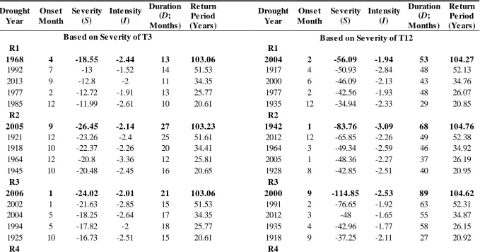
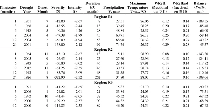
Table 5.2 Ranked drought events based on the severity and intensity of 3- and 12-month timescales. The top 5 events are listed here. The worst droughts are shown in boldface for each region. ... 107
Table 5.3 Top ranked most severe drought events estimated for each timescale... 115
Table 6.1: Mathematical expressions for bivariate copula functions. ... 125
Table 6.2: Kendall’s tau (τ) and an associated p-value of the SPEI, and drought severity, duration and intensity with 13 climate mode indices. Statistically significant correlations are in bold italics and selected for the study are in bold red italics. ... 131
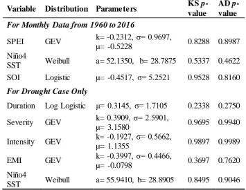
Table 6.3: Marginal distribution parameters and p-values of observed variables. ... 133
Table 6.4: Copula parameters and goodness-of-fit measures of the fitted copula models. ... 136
Table 6.5: Comparison statistics for observed and predicted SPEI for bivariate and trivariate joint copula models. ... 145
Table 6.6: Comparison statistics for observed and predicted duration, and intensity from the bivariate copula models. ... 151
General Acronyms
ANFIS Adaptive Neuro-Fuzzy Inference System ANN Artificial Neural Networks
AWAP Australian Water Availability Project BoM Bureau of Meteorology
CUSUM Cumulative Sum
CSIRO Commonwealth Scientific and Industrial Research Organisation CWT Continuous Wavelet Transform
DEM Digital Elevation Model
DI Drought Index
DVI Drought Vulnerability Indicator GDP Gross Domestic Product
GIS Geographic Information System GWP Global Water Partnership IOD Indian Ocean Dipole
IPO Interdecadal Pacific Oscillation MDB Murray Darling Basin
NAO North Atlantic Oscillation
NSW New South Wales
NT Northern Territory
PAWC Plant Available Water Capacity PDO Pacific Decadal Oscillation
POAMA Predictive Climate Ocean Atmosphere Model for Australia
QLD Queensland
SA South Australia
SAM Southern Annular Mode SEQ Southeast Queensland SOI Southern Oscillation Index SWAT Soil and Water Assessment Tool
VIC Victoria
WA Western Australia
WMO World Meteorological Organization XWT Cross Wavelet Transform
Acronyms for Drought Indices
ADI Aggregated Drought Index API Antecedent Precipitation Index CMI Crop Moisture Index
CSA Cumulative Streamflow Anomaly CSM Computed Soil Moisture
CZI China-Z Index DAI Drought Area Index
DCPA Discrete and Cumulative Precipitation Anomalies DM Drought Monitor
PDSI Palmer Drought Severity Index
PHDSI Palmer Hydrological Drought Severity Index PMAI Palmer Moisture Anomaly Index
PN Percent Normal
RAI Rainfall Anomaly Index RD Rainfall Departure
RDDI Rainfall Decile-based Drought Index RDI Reclamation Drought Index
sc-PDSI Self-Calibrated Palmer Drought Severity Index SMAI Soil Moisture Anomaly Index
SMDI Soil Moisture Deficit Index
SMDDI Soil-Moisture Decile-based Drought Index
SPEI Standardised Precipitation-Evapotranspiration Index SPI Standardised Precipitation Index
SWSI Surface Water Supply Index TWD Total Water Deficit
VCI Vegetation Condition Index
Variable Symbols
P Precipitation WRel1 Upper layer soil moisture
ETo Reference
Evapotranspiration
WRel1End Upper layer end of month aggregate soil moisture
T Temperature D Duration
Tmax Maximum Temperature S Severity
INTRODUCTION
1.1 Background
A drought is a global, natural, and recurring climatic feature that results from a prolonged period of abnormally low rainfall. According to Hewitt (2014), drought ranks first among other natural disasters with numbers of individuals directly affected. It is the least understood climatic feature due to its complex nature, yet it results in on average 6-8 billion USD of annual damage globally (Keyantash and Dracup 2002). The slow development of drought poses difficulty in its detection while the drought preparedness and mitigation solely depends on timely information of the onset, progress and areal extent (Mishra and Singh 2011). Therefore, there is a pressing need to explore new mechanisms for investigating drought characteristics by examining historical events and developing robust predictive and risk evaluative frameworks for the spatial and temporal features. Scientific studies that develop new methods for drought-risk assessments can add new and valuable dimensional information for better preparedness, mitigation, adaptation and regional vulnerability assessment.
extreme droughts (CSIRO 2008a; CSIRO 2008b). Table 1.1 lists the major droughts that occurred in Australia. Increasing population leading to increasing in demand per capita, and a projected increase in the temperature and decrease in rainfall, is likely to make droughts become an issue that is even more relevant. According to the Australian Bureau of Statistics, the national population in Australia is projected to double by 2075 (Statistics 2013). The increase in population size and warming climate can have vast implications on water supply, and therefore, drought studies are very important for identifying ways to lessen the magnitude of impacts that drought may trigger.
Table 1.1: List of major droughts in Australia. After Deo et al. (2015).
Drought Year Descriptions
1895 – 1903
(Federation Drought)
Felt nationwide but was mostly persistent in QLD, inland NSW, SA and central Australia. Sheep numbers reduced to half and cattle numbers declined by more than 40%. The wheat yield dropped from 8 bushels/acre to 2.4 bushels/acre in 1902.
1911 – 1916 Affected nationwide with varying severity.
1918 – 1920 Affected nationwide. 1922 – 1923 and
1926 – 1929
Nationwide with varying severity. 1933 – 1938 Nationwide with varying severity
1939 – 1945
(World War II Drought)
Affected nationwide.
1946 – 1949 Nationwide with varying severity.
1951 – 1952 Pastoral areas were particularly affected in QLD, NT, WA.
1958 – 1968 Most widespread, consistently prominent for long period. Affected nationwide with varying intensity.
1970 – 1973 Affected WA caused by a successive decline in average rainfall.
1976 Affected western NSW and most of VIC and SA due to lack of autumn-winter rains.
The Wimmera Southern Mallee region of Victoria
experienced 80% and 40% reduction in grain and livestock production, respectively.
1991 – 1995 Affected northeastern NSW and much of QLD as a result of lowest levels of rainfall on record. The reservoirs water levels went critically low, the average rural population declined by over 10% while unemployment went up. The estimated loss of the economy was around $A5 billion.
1996 – 2010
(Millennium Drought or “Big Dry”)
A prolonged period of dryness affected much of southern Australia. The drought condition was severe in the densely populated southeast and southwest and affected the Murray-Darling Basin (MDB) severely. Southeast Australia
experienced its lowest 13-year rainfall record since 1865. Agricultural production fell from 2.9% to 2.4% of GDP between 2002 and 2009. It was estimated that drought reduced national GDP by roughly 0.75% between 2006 and 2009 while regional GDP in MDB fell by 5.7% below forecast that accompanied the temporary loss of 6000 jobs between 2007 and 2008.
Other Sources: Wittwer et al. (2002), Year Book Australia, 1988, Australian
1.2 Statement of the Problem
Indisputably, the impact of droughts is devastating to health, economy, ecosystems and urban water supply. Droughts can contribute to decline in human health and increase in mental health problems such as post-traumatic stress and suicidal behaviour (Haines et al. 2006). In fact, the World Meteorological Organization (WMO) has linked drought to 680,000 deaths globally from 1970-2012 (Golnaraghi et al. 2014). In rural affected populations in Australia, droughts can exacerbate mental health issues and increase suicide rates (Alston 2012). Droughts also have severe economic repercussions on agriculture, tourism, employment and livelihood in Australia. For example, between 2002 and 2003, decreases in agricultural production due to drought resulted in 1% reduction in Gross Domestic Product (GDP) (ABS 2004). Carroll et al. (2009) predicted that an increase in drought frequency in the future is likely to have an estimated cost of $5.4 billion annually, reducing GDP by 1% per annum.
Similarly, drought has economic repercussions on Australia’s tourism industry. The reduced visitor days in 2008 in the Murray River region had caused an estimated loss of $70 million (TRA 2010). Drought also significantly impacts on Australia’s ecosystem. During the Millennium Drought, there was a marked decline in water bird, fish and aquatic plant populations in the Murray Darling Basin (MDB) (Leblanc et al. 2012) and loss of 57,000 ha of planted forests (van Dijk et al. 2013). Additionally , droughts can reduce inflows into vital urban water catchments. During the Millenn iu m Drought in southeast QLD, severe water restrictions were implemented where in some areas the average water use declined to 129 litres per person per day, in comparison to a regional consumption of 375 litres under normal (non-drought) operating conditions (Council 2015).
significant issues mentioned above, this study aimed to address the following research gaps to make significant contributions to this study area:
1. Given highly variable climate and prone to climate change effects, a drought monitoring index based solely on precipitation (such as Rainfall Decile-based Drought Index; RDDI) may not reveal the detailed information for drought-risk assessment in Australia. This study, therefore, employed the SPEI to take into account both precipitation and reference evapotranspiration to capture impacts of increased temperatures on water demand, to identify onset and termination points of historical drought, and to estimate their corresponding severity, intensity and duration properties. Additionally , drought is a multi-scalar phenomenon where the timescale over which water deficits accumulate is extremely important and functionally separates meteorological, hydrological and agricultural droughts. There has been a paucity of such analysis for Australian droughts, and therefore, this study characterises droughts on multiple scales. This can enable monitoring and management of different usable water resources. 2. Several large-scale climate drivers, such as the El-Niño Southern
drought-prone regions in Australia. Studies performed elsewhere integrated various physiographic and climatic factors based on certain assumptions that incline towards subjective assessments of droughts. This study has integrated the fuzzy logic theory to provide a mere objective assessment of drought and generate the descriptive drought-risk maps using vulnerability, exposure and hazard indices. As such the subjectivity in the assessment of drought can potentially be minimised.
1.3 Research Aims and Objectives
The aim of this study is to develop a statistical and geospatial-based framework and verify its suitability for drought-risk research with three main objectives. The application on drought-risk management framework is expected to improve the modelling precision for accurate assessment and prediction of drought events using the available hydro-meteorological, climatic and physiographic parameters. Specifically, this study addresses the following three objectives:
(1) To apply the Standardised Precipitation-Evapotranspiration Index (SPEI) for drought assessment by considering jointly the impact of precipitation
and reference evapotranspiration on the water deficit. This objective assesses the relationship between SPEI and other drought-related variables where such comparison is expected to aid in addressing impacts of droughts on agriculture. The SPEI is also applied to estimate the drought return periods for a given severity and intensity amounts, as well as to analyse the multi-scalar properties for drought monitoring. This objective is addressed in Chapters 4 and 5.
(2) To model joint distributions of SPEI and severity-intensity-duration with climate mode indices using multivariate copula functions to examine the risk and
return periods and to emulate conditional probabilistic predictions. This objective evaluates the potential utility of vine copula for studying multivariate associations of SPEI and drought properties with the synoptic scale climate mode indices that act to influence the severity of droughts. The vine copula is also used to develop the probabilistic drought prediction model using the information from climate mode indices. The conditional joint probabilities and joint return periods elucidates the importance of multivariate copula modelling for drought-risk assessment. This objective is addressed in Chapter 6.
(3) To devise an appropriate droughtrisk index by integrating hydro -meteorological and physiographic factors using fuzzy logic algorithms to assess
The three objectives of this study are illustrated in Figure 1.1 below.
Figure 1.1: Three main objectives of this study.
In achieving these objectives, this study hypothesises that: “statistically and spatially explicit drought-risk models can provide sets of information that are useful in planning and developing strategies from the potential effects of extreme drought events to agriculture and availability of water resources”.
Drought-Risk
Drought Monitoring
(SPEI)
[Chapters 4 & 5]
[image:24.595.169.492.113.366.2]Geospatial Modelling (Fuzzy logic)
[Chapter 7]
Statistical Modelling (Copula)
1.4 Significance of the Study
To develop robust drought management strategies, including adaptive and mitigation measures for drought, a framework that can combine multiple intelligent techniques for assessing the drought risk is extremely crucial.
The new knowledge gained from this study can contribute to improving our understanding of the drought characteristics: onset, termination, duration, severity and intensity in the study regions. A framework for drought-risk comprising spatial maps of drought-risk, and joint distribution for drought characteristics with conditiona l return periods and drought predictions, can strongly disseminate drought-risk information and serve as the strong basis for policy and management strategies for drought mitigation and adaptation. The study also presents a novel application of the GIS-based fuzzy logic tool to include various physiographic and hydro-meteorolog ica l parameters that are expected to lessen the amount of subjectivity in drought vulnerability and risk assessments. The techniques evolved from this study can be made applicable to other drought-prone regions globally.
1.5 Organisation of the Thesis
This thesis is organised into eight chapters:
Chapter 1 presents the introductory background to the research, identifies the research problems and significance of the study, and sets out the objectives.
Chapter 2 reviews the subjects of knowledge that are relevant to this study: drought monitoring, drought modelling, and spatial representation of drought-risk. Discussion on existing drought monitoring indices, suitability of the SPEI, copula for probabilist ic drought predictions as well as drought vulnerability and risk assessment is done.
Chapter 3 describes the study area, data and discusses scope and limitation of the study. This chapter serves as the gateway to Chapters 4-7.
Chapter 4 presents the methodology and first set of results in response to the first objective of the study. Here, the SPEI is compared with other precipitation-based drought indices and its selection for this study is justified.
Chapter 5 presents the methodology and second set of results in response to the first objective of the study. Here, the SPEI is evaluated and affirmed its suitability for drought monitoring and characterising purposes.
Chapter 6 presents the methodology and third set of results in response to the second objective of the study. Here, the copula models are used to derive joint distributions of SPEI and drought properties (duration, severity and intensity) coupled with climate mode indices. Subsequently, the development of probabilistic prediction models is made using the joint distribution of multiple variables.
Chapter 7 presents the methodology and fourth set of results in response to the third objective of the study. Here, geospatial representation of drought-risk is made using the fuzzy logic algorithm.
LITERATURE REVIEW
Chapter 1 has presented the overview of the research problem and objectives in regards to the development of the drought-risk assessment framework. This second chapter presents a general review of the literature and then discusses research problems on drought monitoring, modelling and risk-assessment studies in detail. This chapter also establishes the niche for drought-risk management, as well as the relevant sciences and technologies (statistical and geospatial) tools. In brief, Chapter 2 provides the journey towards exploring the relationship of the three major components of this study: (1) characterisation of drought events using the SPEI time series; (2) statistical drought modelling using joint distribution of the SPEI and its properties with climate drivers (climate mode indices); and (3) assessment of drought-risk on temporal and geospatial scales.
2.1 Bureau of Meteorology definitions of drought
The Australian Bureau of Meteorology (BoM) defines meteorological drought as ‘acute water shortage’, which is indicated by the rainfall deficiency for over three months (BoM 2015). The monthly-standardised metric used by BoM to identify drought conditions is the RDDI, which is a measure of rainfall deficiency in terms of
hence does not take into account other variables such as temperature and evaporation that are essential for establishing climatic surface water balance. Figure 2.1 shows the spatial distribution of rainfall in terms of the deciles for part of the Millennium Drought (1/11/2001 to 31/10/2009) in southeast Australia with significant rainfall deficiency.
Figure 2.1: Rainfall deciles for the period 1 November 2001 to 31 October 2009 [Source: Australian Bureau of Meteorology].
characteristics (e.g., duration, severity, intensity) in order to understand the phenomenon even better and develop more strategic mitigation plans.
2.2 Drought Monitoring
Why is it important to monitor droughts? Droughts are a normal part of the climate system and occur in virtually all climate regimes globally, including deserts that are naturally arid. According to Wilhite (2000), drought is the most costly natural disaster on a year-to-year basis, with impacts being extremely significant and widespread, affecting many people and economic sectors at any one time. The areas affected by droughts are typically larger than any other hazards. The slow onset of droughts allows time to observe changes in precipitation and status of surface and groundwater supply in a region over time. To help track of the drought condition, drought indicators or indices are often used, and these tools vary depending on region and season.
Like other hazards, droughts can be categorised in terms of location, onset, duration, severity, intensity, areal extent and cessation. A range of hydro-meteorological processes that suppress the precipitation and/or limit the surface or groundwater availability resulting in soil moisture deficiency can cause droughts. Therefore, monitoring of droughts is crucial for preparedness and proactive actions in mitigating the impacts. As such, the indicators and indices help identify and evaluate the characteristics of droughts. To monitor different aspects of the hydrologic cycle, a variety of indicators and indices are required. As droughts evolve, the impacts can vary by region and by season, therefore, for drought early warning system, it is important that indicators and indices accurately reflect and represent the impacts.
and demand of economic goods during drought conditions. The latter three drought categories lag behind meteorological drought that are all linked to it. A better understanding of the meteorological category of drought can help understand the impacts of other category of events. There is a general consensus that the slow development of drought, often called “creeping nature of the event” poses difficulty in its detection. From the same standpoint, drought preparedness and mitigation plans solely rely on the timely information about their onset, progression and areal extent or coverage (Mishra and Singh 2011; Morid et al. 2006). This very important information is obtained from drought monitoring that is usually performed using Drought Indices, hereafter called DIs. This investigation tests the suitability of standardised precipitation-evapotranspiration index (SPEI) for the first time as the novel application for monitoring and assessing characteristics of drought events in south-east Queensland, Australia.
2.2.1 Existing indices for drought monitoring
Several drought indicators and indices have evolved over the years. Scientists, stakeholders and decision-makers may use indicators and/or indices for drought monitoring purposes. It is important to understand what is meant by the terms ‘indicators’ and ‘indices’. According to WMO and GWP (2016), the indicators are “variables or parameters used to describe drought conditions. Examples include precipitation, temperature, streamflow, groundwater and reservoir levels, soil moisture and snowpack”, whereas indices are “typically computed numerical representations of drought severity, assessed using climatic or hydro-meteorological inputs including the indicators listed above”. As opposed to the indicators, DIs are generally standardised metrics that simplify the complex relationships and provide useful communicatio n tools for diverse audiences and users. Indices are used to quantify the drought characteristics that enable drought early warning (Kogan 2000) and drought risk (Hayes et al. 2004) analysis, which in turn allows improved preparedness and contingency planning.
levels, while some indices represent aggregate nature of meteorological, hydrologica l and agricultural droughts. There is also a considerable number of indices that use remote-sensing imagery, for e.g., to detect vegetation health as an indicator of droughts. DIs have a wide range of applications, including drought monitoring , prediction, quantitative assessment, and developing management strategies under current climate (Karl 1983) as well as under climate change associated with global warming (Le Houérou 1996).
Table 2.1: Commonly used drought indices. After WMO and GWP (2016). Index Name Variables
Needed
Applications Strengths Weaknesses
Percent of Normal (PN) Werick et al. (1994)
P Can be used for
identifying and monitoring meteorological,
agricultural, and hydrological droughts.
A popular method that is quick and easy to calculate with basic mathematics.
What is normal for an area is a calculation that some will confuse with mean or average precipitation. It is hard to compare different climate regimes with each other, especially those with defined wet and dry seasons.
Standardised Precipitation Index (SPI) McKee et al. (1993)
P Can be calculated at various timescales that allows for applications across meteorological, agricultural, and hydrological drought events. Meteorological drought events may focus on SPI values of 3 months or less; agricultural
drought events, values of 6 months or less; and
hydrological droughts, values of 12 months or longer, give or take. The SPI can also be calculated on gridded precipitation data sets, which allows for
Using only precipitation data is the greatest strength of the SPI, as it makes it very easy to use and calculate the index.
It is applicable in all climate regimes.
It can be computed for short periods of record, which contain missing data, is also valuable for those regions that may be data poor or lacking long-term, cohesive data sets.
The program used to calculate the SPI is easy to use and readily available.
The ability to be calculated over multiple timescales
With precipitation as the only input, the SPI falls short when accounting for the temperature component, which is important to the overall water balance and water use of a region. This drawback can make it more difficult to compare events of similar SPI values but different temperature scenarios. The
a wider scope of users than those just working with station-based data. Standardised
Precipitation-Evapotranspir ation Index (SPEI) Vicente-Serrano et al. (2010)
P, T With the same versatility observed with the SPI, the SPEI can be used to identify and monitor conditions associated with meteorological,
agricultural, and hydrologic drought conditions.
The inclusion of temperature data along with precipitation allows the SPEI to account for the impact of temperatures on a drought situation. The output of the SPEI is applicable for all climate regimes, with the results being comparable side by side as the results are standardised. With the use of temperature data, the SPEI is an ideal index when looking at the impact of climate change on model output under various future scenarios.
The requirement of needing a serially complete data set for both
temperature and precipitation may limit the use of the SPEI because the available data may not allow it to be used. Being a monthly index,
rapidly developing drought situations may not be identified quickly.
Rainfall Anomaly Index (RAI) Van Rooy (1965)
P Addresses meteorological, agricultural, and
hydrological drought, as the RAI is flexible in that it can be analysed at various timescales.
Ease in calculations with a single input (precipitation) that can be analysed on monthly, seasonal, and annual scales.
The index requires no missing data, and a serially complete data set with estimates of missing values is needed. Variations within the year need to be small compared to the temporal variations. Missing data need to be accounted for to create a serially complete data set.
Rainfall Decile based Drought Index (RDDI) Gibbs and Maher (1967)
P With the ability to look at different timescales and time steps, deciles can be used in meteorological, agricultural, and hydrological drought situations.
With a single variable being considered, the methodology is simple and flexible for many situations. With clearly defined thresholds, the current data is put into a historical context and drought status can be recognized. Useful in both wet and dry situations.
As with other indicators that only use precipitation, the impact of
many wet and dry periods will be included in the distribution. Palmer
Drought Severity Index (PDSI)
Palmer (1965)
P, T, AWC Developed mainly as a way to identify
agricultural droughts, the PDSI has been used in identifying and monitoring meteorological and
hydrological droughts as well. With the longevity of the PDSI, there are numerous examples of how the index has been utilized over the years.
The PDSI is used around the world and the code and output are widely available. With the legacy of the index, the scientific literature is full of papers related to the PSDI. The use of soils data and a total water balance methodology makes the PSDI quite robust in identifying drought.
The need for serially complete data will make using the PDSI
problematic for some. The PDSI has a timescale of approximately 9 months, which leads to a lag in identifying drought conditions based upon the simplification of the soil moisture component within the calculations. This lag may be up to several months, which is a drawback when trying to identify a rapidly emerging drought situation. Seasonal issues also exist, as the PDSI does not handle frozen precipitation or frozen soils well.
Self-Calibrated Palmer Drought Severity Index (sc-PDSI) Wells et al. (2004)
P, T, AWC Can be applied to meteorological, hydrological and agricultural drought.
Is specific to the station location allowing for more accurate comparisons between regions.
Can be calculated on different timescales.
China Z Index (CZI)
Kendall and Stuart (1977)
P Similar to the SPI, in which both wet and dry events can be monitored over multiple timescales. Drought applications would apply to meteorological, agricultural, and hydrological droughts.
Simple calculations, which can be computed for several time steps. Can be used for both wet and dry events. Allows for missing data, similar to the SPI.
The Z-Score data does not require adjusting the data by fitting them to the Gamma or Person Type II
distributions, and it is speculated that because of this, shorter timescales may not be represented as well compared to the SPI.
Crop Moisture Index
Palmer (1968)
P, T Used to monitor droughts where agricultural impacts are the primary concern.
The output is weighted, making it possible to compare different climate regimes. Responds quickly to rapidly changing conditions.
It was developed specifically for the grain-producing region in the United States, therefore CMI may show a false sense of recovery from long-term drought events, as
improvements in the short term may be insufficient to offset long-term issues.
Soil Moisture Deficit Index (SMDI) Narasimhan and Srinivasan (2005)
Mod Useful for identifying and monitoring short-term drought affecting agriculture.
Takes into account full profile as well as different depths, making it adaptable to different crop types.
Calculations are based upon the output from SWAT model and there are auto-correlation concerns when all depths are being used.
Reclamation Drought Index (RDI)
P, T, S, RD, SF
Used mainly to monitor water supply for river basins.
Specific to each basin.
Accounts for temperature effects on climate.
Calculations are made for the
Weghorst
(1996) Standardised scale allows for monitoring
of wet and dry conditions.
Putting together all inputs in
operational setting may cause a delay in data production.
Surface Water Supply Index (SWSI) Shafer and Dezman (1982)
P, RD, SF, S
Used to identify droughts associated with
hydrological fluctuations.
Taking account of full water resources of a basin provides a good indication of the overall hydrological health of particular basin or region.
The index has to undergo recalculation when data source changes or inclusion of additional data, making it difficult to construct a homogeneous time series.
Calculations vary between basins, making it difficult to compare. Effective
Drought Index (EDI)
Byun and Wilhite (1999)
P The EDI is a good index for operational monitoring of both meteorological and agricultural drought
situations because its calculations are updated daily.
With only a single input needed for calculations, it is possible to calculate the EDI at any location where precipitation is recorded. Support documentation
explaining the processes are available for the program. The EDI also is standardised so that outputs from all climate regimes can be compared. The EDI is effective in identifying the beginning, ending, and duration of drought events.
With only precipitation accounted for, the impact of temperatures on drought situations is not directly acknowledged. With using daily data, it may be difficult to use the EDI in an operational situation as daily updates to input data may not be possible.
2.2.2 Selection of indicators and indices
Just as there is no single definition of drought, there is no single indicator or index that is suitable for all drought types, climate regimes and sectors affected by droughts. Also, the simplest indicator/index may not necessarily be the best or most applicable for the region. The drought analyst must feed in many factors before determining which indicator, index (or both) to use for the particular need or application. Some of the questions that the drought analyst may need to consider include: (1) is the indicator/index sensitive to climate, space and time in order to determine the accurate onset and cessation of drought? (2) does the indicator/index allow for timely detection of drought in order to trigger appropriate communication and coordination of drought mitigation or response actions? (3) are data and resultant indicator/indices reliable?
i.e., are the data available for a long period of record in order to understand historical droughts? and (4) is the indicator/index easy to implement? (WMO and GWP 2016). For the evaluation of meteorological DIs, Keyantash and Dracup (2002) suggested considering six criteria: robustness, tractability, transparency, sophistication , extendability and dimensionality.
2.2.3 Comparison of existing drought indices for quantifying drought events
Table 2.2: Studies comparing various drought indices.
Study Indices Compared
Notes and Outcomes Recommendations
Mpelasoka et al. (2008) Australia RDDI and SMDDI
Indices were used to assess future drought events over Australia under global warming attributed to low and high greenhouse gas emission scenarios for 30-year periods, centred on 2030 and 2070.
Both indices showed a general increase in drought frequency associated with global warming.
ETo and T were important in determining the severity of droughts and be even more as climate changes in warmer conditions.
SMDDI appeared to be more relevant to resource management as it accounts for ‘memory’ of water status.
Considering soil-moisture delays tend to indicate realistic severity and persistence for drought events, meteorological drought indices (i.e., RDDI) were inadequate for reliable assessment of drought.
Morid et al. (2006) Tehran, Iran
Decile Index, PN, SPI, CZI, MCZI, Z-Score and EDI
The study compared the performance of seven drought indices for 32-years of data.
SPI, CZI and Z-Score performed similarly with regards to drought identification and respond slowly to drought onset. Decile Index appeared to be very responsive to rainfall events of a particular year but had inconsistent spatial and temporal variation.
MCSI and PN were not recommended for drought
monitoring as they were found to declare ‘extreme drought’ conditions unreasonably frequently.
SPI and EDI were able to detect drought onset, spatial and temporal variation consistently, thus may be recommended for operational drought monitoring. EDI was found to be more responsive to the emerging drought and overall
Dogan et al. (2012) Konya, Turkey
PN, RDDI, Z-Score, CZI, SPI and EDI
The study compared drought indices under different climatic conditions and on 18 different timescales.
Results showed median timescales were essential for future studies while 1-month timescale was irrelevant in arid/semi-arid regions where rainfall deficiency was common. Drought indices for 6-, 9-, and 12-month timescales were found essential for long-term drought studies, while 1-month drought indices not to be used for comparison studies for the recommendation of an index.
EDI was best correlated with other indices on all timescales and was preferable for monitoring long-term droughts in arid/semi-arid regions.
Barua et al. (2010) Yarra River Catchment in Victoria, Australia.
ADI, SPI, SWSI The study attempted to show the significance of Aggregated Drought Index (ADI) by considering significant components of the water cycle. The principal component analysis was used to consider hydro-meteorological variables that describe fluctuations in hydrologic cycles. The ADI was compared with SPI and SWSI.
ADI incorporated precipitation, evapotranspiration,
streamflow, surface reservoir storage, soil moisture content. The main advantage of ADI included its assessment of droughts from aggregate perspective of meteorological, hydrological and agricultural water shortages.
ADI was found to be more robust than SPI and SWSI where ADI was able to detect historical droughts more clearly.
Lloyd-Hughes and
SPI and PDSI The study compared drought indices on timescales 3, 6, 9, 12, 18 and 24 months for the period 1901-1999.
Saunders (2002) Europe
Trends in SPI and PDSI values indicated the proportion of Europe experiencing extreme and/or moderate drought conditions changed insignificantly during the 20th century.
Overall, SPI provided better spatial standardization than PDSI. SPI was recommended for it is a simple and effective tool for the study of European droughts. Dubrovsky et al. (2009) 45 stations in the Czech Republic
SPI and PDSI The study applied relative SPI and PDSI to assess climate-change impacts on drought conditions over 1961-2000 and 2060-2099 periods.
PDSI exhibited the widest spectrum of drought conditions across Czech, in part because it depended not just on precipitation (as does SPI) but also on temperature. In future climate analysis, SPI-based drought risk closely followed modelled changes in precipitation while PDSI indicated an increase in drought-risk.
The study concluded on PDSI being more appropriate for use over SPI in assessing the potential impact of climate change on future droughts.
Pandey et al. (2008) Orissa, India
SPI and EDI, Decile Index, Departure from long-term mean and median
This study has used SPATSIM for drought analysis on monthly (SPI, Decile Index, Departure from long-term mean and median) and DWRAM software for daily (EDI) bases. All SPI, EDI and annual deviation from mean showed a similar trend of drought severity.
EDI better-represented droughts in any area over other DIs.
Decile index was found to be not suitable.
Heim Jr (2002)
Munger’s, Kincer’s, Marcovitch’s,
This study showed how the insights into the understanding of droughts have changed over past hundred years.
USA Blumenstock’s indices, API, MAI, PDSI, PHDI, CMI, K-BDI, SWSI, SPI, VCI, DM
landmark development, and that indices must address the total environmental moisture status. The Drought Monitor (DM) index has shown a considerable progress with comprehensive, objective national drought index.
Keyantash and Dracup (2002) Oregon, USA Meteorological: DCPA, RD, PDSI, DAI, RAI, SPI Hydrological: TWD, CSA, PHDSI, SWSI Agricultural: CMI, PMAI, CSM, SMAI
This study carried out a comprehensive evaluation of most prominent drought indices in meteorological, hydrological and agricultural categories using the weighted set of six criteria: robustness, tractability, transparency, sophistication, extendability, and dimensionality.
Drought indices were ranked in terms of usefulness for the assessment of drought severity, for two test regions.
The evaluation scores showed overall superior drought indices were rainfall deciles (RD), total water deficit (TWD) and computed soil moisture (CSM) for meteorological, hydrological and agricultural drought, respectively.
Jain et al. (2015) Ken River Basin, India
SPI, EDI, Z-Score, CZI, RD, RDDI
DIs on five timescales (1, 3, 6, 9 and 12-months) were compared with each other (monthly) and with EDI (daily). 1-month timescale may produce erroneous estimates of drought duration and 9-month timescale was best correlated.
RD and RDDI were not recommended due to their disagreement on estimates of drought duration and frequencies with other indices.
2.2.4 Standardised Precipitation-Evapotranspiration Index (SPEI) for drought monitoring
In the current era, it is a common knowledge that drought events, as prolonged climatological deficits in precipitation, continue to foster serious hydrologica l imbalances (Wilhite and Glantz 1985), and trigger agricultural, health and environmental repercussions (Wilhite et al. 2014). Objective characterisation of drought in terms of duration, severity, intensity (D-S-I) properties and the spatial extent and inter-arrival times is naturally difficult since drought exhibits a creeping nature with a slow emergence profile. Therefore, DIs that provide normalised comparisons of drought in climatologically diverse regions, are normally applied to monitor a drought event. As a supply-side assumption, droughts are primarily driven by precipita tion variability, however, many DIs neglect the importance of the variables other than precipitation that can act to exacerbate the drought impacts. This study explores, for the first time in the drought-prone zone of southeast Queensland (SEQ), the utility of the SPEI for drought assessments. The SPEI (Vicente-Serrano et al. 2010) has been adopted as a multi-scalar and a relatively new metric, utilising precipitation and estimated reference evapotranspiration for statistical quantification of drought characteristics.
The PDSI has been widely adopted for it utilises precipitation, temperature , soil water recharge, runoff, water loss from soil and soil water capacity (Lloyd-Hughes and Saunders 2002) to examine water balance whilst assessing the moisture status in a comprehensive (and hydrologically-relevant) manner. However, it carries some challenges and limitations. While the PDSI is an ideal metric for an assessment of hydrological drought, its high demand for input data and fundamental assumptions make it too complex to account for the physical and biological factors associated with a drought event (Felch 1978). Also, the PDSI appears to be unsuitable for many climatic regions (including Australia) due to its normalisations based on limited comparisons and unsolidified justification by physical and statistical basis (Alley 1984; Gibbs and Maher 1967; Guttman et al. 1992; Keyantash and Dracup 2002). General applicability of the scaling process with a limited number of empirical factors becomes a constraint of PDSI to be applied outside the USA, as questioned by some studies (e.g., (Dai 2011)). A similar sentiment was shared by Redmond (2002), indicating that the creator of PDSI did not intend to apply PDSI beyond the Great Plains in the central USA. Moreover, studies showed that PDSI underperforms for climatic regions with extreme variability of rainfall and run-off, and this is especially true for Australia (Burke et al. 2006). To avoid abovementioned empirical relationships, Wells et al. (2004) developed the self-calibrated PDSI (sc-PDSI). Nevertheless, the necessary data requirement in the sc-PDSI was not reduced.
conditions. Other advantages include less data requirement, flexibility, and simple computation. These accord to the viewpoint of Keyantash and Dracup (2002) that a drought metric must be simple, clear, comprehensible and statistically robust, and also be independent of the climatic characteristics (i.e., standardised) to be comparable in the wider temporal and spatial domains across geographically diverse regions. However, the unavailability of ETo data for computing the SPEI can be a potential drawback since its estimation requires multiple input variables (e.g., humidity, solar radiation, and wind speed information) for the recommended FAO-56 Penman-Monteith technique (Allen et al. 1998).
Despite its infancy in the hydrologic research community, many case studies performed outside of Australia have applied the SPEI for drought assessment and demonstrated its statistical correlation with hydro-meteorological variables that has drought impacts in such diverse climatic regions. For example, the SPEI was used for drought variability studies (Das et al. 2016; Li et al. 2012; Paulo et al. 2012; Potop 2011), hydrological impact assessments, agricultural drought studies, impact of drought on ecological systems (Barbeta et al. 2013; Cavin et al. 2013; Martin-Benito et al. 2013; Toromani et al. 2011; Vicente-Serrano et al. 2013) as well as in the monitoring of drought events (Fuchs et al. 2012). However, to date, only three studie s have applied this index for drought studies in Australia (Dayal et al. 2018; Dayal et al. 2017; Deo and Şahin 2015). Therefore, the successful application of SPEI elsewhere and its features relevant to Australia’s climate, i.e., incorporation of evapotranspiration as a measure of water demand, would add to new insights on understanding Australian droughts better and be made recommended for drought monitoring purposes.
2.3 Drought Modelling
2.3.1 Drought forecasts and predictions
Drought forecasting is a critical component of drought hydrology that plays a major role in the risk management, drought preparedness and mitigation. There has been a significant amount of work done on modelling various aspects of drought, such as estimation and prediction of its severity and duration. However, the major challenge has been to develop techniques to forecast drought onset and termination points for months or years in advance (Mishra and Singh 2011). Several studies have predicted drought or its properties using regression, probability, machine learning and hybrid models. For instance, Kumar and Panu (1997) developed a regression model to predict grain yield that would in turn aid in the assessment of agricultural drought severity as a function of time. In another study, Leilah and Al-Khateeb (2005) employed statistical procedures to study the relationship between wheat grain and its components under drought conditions of Saudi Arabia. Liu and Juárez (2001) used multiple linear regression techniques to predict drought onset using El-Niño Southern Oscillation (ENSO) indices (independent variables) and satellite-recorded Normalised Difference Vegetation Index (dependent variables). The multiple regression predicts one variable from two or more independent variables, i.e.,
where is the dependent variable (predictand such as drought index) and , and are independent variables (predictors such as rainfall, streamflow, and soil moisture) and and are constants. There are several limitations albeit regression models been a commonly used method. One major limitation is the assumption of linearity between predictor (e.g., climate mode indices) and the predictand (e.g.,
drought index) that makes it less capable for long-term forecasting. This is due to the highly stochastic nature of the environmental factors where the linear relationship may not hold true between variables. The other limitation is the difficulty in understanding causal mechanisms and multicollinearity, i.e., the conceptual framework of the regression models (Mishra and Singh 2011).
The probabilistic models are useful for predicting droughts due to their complex nature and the ability to quantify uncertainties associated with hydro -meteorological variables. The Markov chain models have been commonly used for drought predictions. A Markov chain is a stochastic process with a property that at the 3 2 1 cX dX
bX a
Y
Y X1 X2
X3
c b
value of the process at any time , the would only depend on its value at a time , and not in the sequence of values , which can be written as (Haan 2002):
Prob
= Prob
(2.1)
The Prob is the conditional probability that gives the probabilit y that the process at a time will be in “state j”, given that at a time , the process was in “state i” (Mishra and Singh 2011). The Prob is commonly termed as one-step transition probability that is basic to the structure of Markov chains.
The study of Gabriel and Neumann (1962) was among the first to apply Markov chain models for dry spell analysis. Lohani and Loganathan (1997) used a non-homogenous Markov chain model based on PDSI to characterise the stochastic behaviour of droughts for an early warning system. This characterisation was in the form of a decision tree enumerating all possible sequences of drought progression , which was useful for drought management. Bogardi et al. (1994) described that the statistical properties of droughts can be obtained by conditioning monthly drought indices on large-scale atmospheric circulation patterns, which can predict droughts under the chang