Identification of vehicle axle loads from bridge responses using preconditioned least square QR-factorization algorithm

1

Identification of vehicle axle loads from bridge responses using

preconditioned least square QR-factorization algorithm

Zhen Chen

_{, Tommy H.T. Chan}

_{, Andy Nguyen}

_{, Ling Yu}

a

School of Civil Engineering and Communication, North China University of Water Resources and Electric Power, Zhengzhou 450045, China

b _{School of Civil Engineering and Built Environment, Queensland University of Technology}

(QUT), Brisbane 4000, Australia

c _{School of Civil Engineering of Surveying, University of Southern Queensland (USQ),}

Springfield Central, 4300, Australia

d _{MOE Key Lab of Disaster Forecast and Control in Engineering, Jinan University,}

Guangzhou 510632, China

Abstract: This paper develops a novel method for moving force identification (MFI) called preconditioned least square QR-factorization (PLSQR) method. The algorithm seeks to

reduce the impact of identification errors caused by unknown noise. The biaxial moving

forces travel on a simply supported bridge at three different speeds is used to generate

numerical simulations to assess the effectiveness and applicability of the algorithm. Results

indicate that the method is more robust towards ill-posed problem and has higher

identification precision than the conventional time domain method (TDM). In addition, the

robustness and ill-posed immunity of PLSQR are directly affected by two kinds of

regularization parameters, namely, number of iterations 𝑗𝑗 and regularization matrix 𝐋𝐋.

Compared with the standard form of least square QR-factorization (LSQR), i.e., the

regularization matrix 𝐋𝐋 being the identity matrix 𝐈𝐈_𝒏𝒏, the PLSQR with the optimal number of

iterations 𝑗𝑗 and regularization matrix 𝐋𝐋 has many advantages on MFI and it is more suitable

for field trials due to better adaptability with type of sensors and number of sensors.

Keywords: moving force identification; preconditioned least square QR-factorization; time domain method; regularization parameter; preconditioner

1. Introduction

The knowledge of dynamic loads acting on bridges is always required to ensure the safety

and reliability of bridges. This information on traffic loading can enable efficient and

economical management of transport networks and is becoming a valuable tool for bridge

safety assessment [1].

The technique of moving force identification (MFI) on bridges is to solve an inverse

problem through the dynamic characteristics of vehicle-bridge system and the measured

responses of bridges, which is very different from the forward problem. Force reconstruction

techniques are often associated with an ill-posed problem due to the recovery of the input of a

*_{Corresponding author at: School of Civil Engineering and Communication, North China University of}

Water Resources and Electric Power, 36 Beihuan Road, Zhengzhou 450045, PR China

2

dynamic system with influential noise, which leads to the reconstruction results in inaccurate

or non-unique solutions [2].

There are four important indirect moving force identification methods developed by Chan

et al [3-6], which have been incorporated into a moving force identification system and then

evaluated by experimental verification in laboratory and field applications [7]. Comparisons

show that all these four methods have acceptable accuracy; but the identification results from

the time domain method (TDM) and the frequency-time domain method (FTDM) are better

than those from the interpretive method I (IMI) and the interpretive method II (IMII). The

TDM was widely adopted because of its high precision and rigorous theory, which can be

used to identify the load history of each axle of a vehicle passing a bridge without interrupting

the flow of traffic. Zhu and Law [8-10] extended the TDM to several different bridge types.

Chan and Ashebo [11] extended the TDM to continuous bridge by considering the responses

of only one selected span from the continuous bridge. Yu and Chan [12] proposed a method

of moments (MOM) algorithm which improved the efficiency compared with the existing

TDM. However, it was still found that the identification results of improved methods based

on TDM suffer large deviation from real load during the local period of the vehicle crossing

the bridge, since the nature of the MFI is ill-posed [13].

In the last decade, some novel techniques have been presented for MFI. Dowling et al. [14]

utilized the first order regularization method to calculate the moving force from bridge strain

responses. Berry et al. [15] presented the theoretical developments of identifying local

dynamic transverse forces on the surface of a thin plate based on the virtual fields method. Li

et al. [16] proposed a force identification algorithm based on wavelet multi-resolution

analysis. Most of the new methods have noise immunity but ill-posedness should not be

ignored. To overcome the ill-posedness of MFI, regularization methods used to be utilized by

converting ill-posed to well-posed and these conditions can be physical or mathematical [2].

Some researchers introduced Tikhonov regularization approach to overcome ill-posedness

problems in MFI, as long as the optimal regularization parameter can be correctly chosen.

Pinkaew [17] adopted an updated static component (USC) technique to overcome

vehicle-bridge parameter sensitivity issues such as the vehicle speed. González et al. [18] proposed a

new bridge weigh in motion algorithm to reduce the dynamic uncertainty of bridge responses.

Mao et al. [19] presented an improved state space method to deal with the ill-posedness

problem. Ronasi et al. [20] added the traditional Tikhonov regularization method within the

numerical framework to reduce the sensitivity to noise of wheel-rail contact force

identification. Law et al. [21-23] proposed and an iterative regularization method for

structural damping identification and damage identification when noise effect is included in

the measurements. Ding et al. [24] proposed a discrete force identification approach based on

average acceleration discrete algorithm. Feng et al. [25] introduced a Bayesian inference

3

proposed a regularized cubic B-spline collocation (CBSC) method to mitigate the ill-posed

problem. Liu et al. [28-31] proposed a series of new methods for MFI based on Tikhonov

regularization such as time-domain Galerkin method, improved regularization method and the

shape function method based on moving least square fitting.

In linear algebra, the least square QR-factorization (LSQR) is an iterative method similar in

style to the well-known conjugate gradients (CG) as applied to the least squares problem

[32,33]. Benbow [34] extended LSQR with similar preconditioned Krylov methods for

solving augmented linear systems in a generalized least squares problem. Jacobsen and

Hansen [35] presented a subspace preconditioned LSQR for the solution of discrete linear

ill-posed problem. Reichel et al. [36,37] presented a generalization of LSQR that allowed the

choice of an arbitrary initial vector for the solution subspace. Karimi and Zali [38] proposed a

block preconditioned least squares (BPLS) and a block preconditioned global least squares

(BPGLS) algorithms to solve the linear system of equations with block partitioned coefficient

matrix and multiple linear system of equations. Arridge et al. [39] derived a factorization-free

preconditioned LSQR algorithm (MLSQR) for solving large-scale linear inverse imaging

problems.

As mentioned earlier, out of many iterative methods for solving the linear algebraic

equation, LSQR is a popular iterative method for the solution of large linear systems of

equations and least-squares problems [36]. In this paper, based on the LSQR technique, a

preconditioned least square QR-factorization (PLSQR) regularization method is proposed for

MFI by choosing proper regularization parameter, such as the number of iterations and the

regularization matrix. The numerical simulation results show that the PLSQR has excellent

ill-posed immunity and high-quality adaptability with different sensors. These advantages of

PLSQR are practical to the field trials of MFI.

2. Background of theory

2.1. Moving force identification by time domain method (TDM)

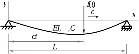
As shown in Fig.1, a moving force 𝑓𝑓(𝑡𝑡) passes over a simply supported Bernoulli-Euler

beam at a constant speed 𝑐𝑐. The span of the beam is 𝐿𝐿 and viscous damping is 𝐶𝐶. The mass

per unit length of the beam is 𝜌𝜌 and flexural stiffness is 𝐸𝐸𝐸𝐸. The dynamic equation of

vehicle-bridge system in modal coordinate 𝑞𝑞_𝑛𝑛(𝑡𝑡) can be expressed as 𝑞𝑞̈𝑛𝑛(𝑡𝑡) + 2𝜉𝜉𝑛𝑛𝜔𝜔𝑛𝑛𝑞𝑞̇𝑛𝑛(𝑡𝑡) +𝜔𝜔𝑛𝑛2_{𝑞𝑞𝑛𝑛(𝑡𝑡) =} 2

𝜌𝜌𝜌𝜌𝑝𝑝𝑛𝑛(𝑡𝑡)，(n = 1,2, … ,∞) (1)

where 𝜔𝜔𝑛𝑛=𝑛𝑛2𝜋𝜋2 𝜌𝜌2 �

𝐸𝐸𝐸𝐸

𝜌𝜌 is the nth modal frequency;𝜉𝜉𝑛𝑛= 𝐶𝐶

4

f(t)

EI,

ρ

,C

c y

x

L ct

Fig.1. Dynamic model of moving vehicle and simply supported beam

The deflection 𝑣𝑣(𝑥𝑥,𝑡𝑡) and the bending moment 𝑀𝑀(𝑥𝑥,𝑡𝑡)of the simply supported beam at

point 𝑥𝑥 and time 𝑡𝑡 in time domain can be obtained as Law et al. [4]

𝑣𝑣(𝑥𝑥,𝑡𝑡) =�_{𝜌𝜌𝐿𝐿𝜔𝜔}2

𝑛𝑛′ ∞

𝑛𝑛=1

sin𝑛𝑛𝑛𝑛𝑥𝑥_{𝐿𝐿 � 𝑒𝑒}−𝜉𝜉𝑛𝑛𝜔𝜔𝑛𝑛(𝑛𝑛−𝜏𝜏)_sin𝜔𝜔

𝑛𝑛′(𝑡𝑡 − 𝜏𝜏)sin𝑛𝑛𝑛𝑛𝑐𝑐𝜏𝜏_{𝐿𝐿 𝑓𝑓}(𝜏𝜏)𝑑𝑑𝜏𝜏 𝑛𝑛

0

(2)

𝑀𝑀(𝑥𝑥,𝑡𝑡) =−𝐸𝐸𝐸𝐸𝜕𝜕2_{𝜕𝜕𝑥𝑥}𝜈𝜈(𝑥𝑥₂,𝑡𝑡)=�2𝐸𝐸𝐸𝐸𝑛𝑛_{𝜌𝜌𝐿𝐿3}2

∞

𝑛𝑛=1

𝑛𝑛2

𝜔𝜔𝑛𝑛′sin

𝑛𝑛𝑛𝑛𝑥𝑥

𝐿𝐿 � 𝑒𝑒−𝜉𝜉𝑛𝑛𝜔𝜔𝑛𝑛(𝑛𝑛−𝜏𝜏)sin𝜔𝜔𝑛𝑛′(𝑡𝑡 − 𝜏𝜏)sin 𝑛𝑛𝑛𝑛𝑐𝑐𝜏𝜏

𝐿𝐿 𝑓𝑓(𝜏𝜏)𝑑𝑑𝜏𝜏

𝑛𝑛

0

(3)

where 𝜔𝜔_𝑛𝑛′ =𝜔𝜔_𝑛𝑛�1− 𝜉𝜉_𝑛𝑛2.

The MFI from bending moment responses by TDM can be expressed as

𝐁𝐁 ∙ 𝐟𝐟=𝐌𝐌 (4) where𝐁𝐁 ∈ 𝐑𝐑(𝑁𝑁−1)×(𝑁𝑁𝐵𝐵−1)_, 𝐟𝐟 ∈ 𝐑𝐑(𝑁𝑁𝐵𝐵−1) _and 𝐌𝐌 ∈ 𝐑𝐑(𝑁𝑁−1)_{. Definition the time interval is} ∆𝑡𝑡_{, the} number of sample points is 𝑁𝑁+ 1 and 𝑁𝑁𝐵𝐵 = 𝜌𝜌

𝑛𝑛∆𝑛𝑛.

Similarly, the acceleration 𝑣𝑣̈(𝑥𝑥,𝑡𝑡) of the simply supported beam at point 𝑥𝑥 and time 𝑡𝑡 in

time domain can be expressed as

𝑣𝑣̈(𝑥𝑥,𝑡𝑡) =�_{𝜌𝜌𝐿𝐿}2 sin𝑛𝑛𝑛𝑛𝑥𝑥_𝐿𝐿 ∞

𝑛𝑛=1

[𝑓𝑓(𝑡𝑡)sin𝑛𝑛𝑛𝑛𝑥𝑥_𝐿𝐿 +� ℎ̈𝑛𝑛(𝑡𝑡 − 𝜏𝜏)𝑓𝑓(𝜏𝜏)sin𝑛𝑛𝑛𝑛𝑐𝑐𝜏𝜏_{𝐿𝐿 𝑑𝑑𝜏𝜏}] 𝑛𝑛

0

(5) where ℎ̈_𝑛𝑛(𝑡𝑡) = 1

𝜔𝜔𝑛𝑛′ 𝑒𝑒

−𝜉𝜉𝑛𝑛𝜔𝜔𝑛𝑛𝑛𝑛× {[(𝜉𝜉_𝑛𝑛𝜔𝜔_𝑛𝑛)2− 𝜔𝜔_𝑛𝑛′2] sin𝜔𝜔_𝑛𝑛′𝑡𝑡+ (−2𝜉𝜉_𝑛𝑛𝜔𝜔_𝑛𝑛𝜔𝜔_𝑛𝑛′) cos𝜔𝜔_𝑛𝑛′𝑡𝑡}_.

The MFI from acceleration responses by TDM can be expressed as

𝐀𝐀 ∙ 𝐟𝐟=𝐕𝐕̈ (6) where 𝐀𝐀 ∈ 𝐑𝐑𝑁𝑁×(𝑁𝑁𝐵𝐵−1)_,𝐟𝐟 ∈ 𝐑𝐑(𝑁𝑁𝐵𝐵−1) _and 𝐕𝐕̈∈ 𝐑𝐑𝑁𝑁_.

Likewise, the MFI from bending moment and acceleration combination responses by TDM

can be expressed as

�𝐁𝐁_𝐀𝐀/_/‖𝐌𝐌‖_{�𝐕𝐕̈��}×𝐟𝐟=�𝐌𝐌_𝐕𝐕̈/_/‖𝐌𝐌‖_{�𝐕𝐕̈� �} (7)

where ‖∙‖ is the norm of the vector.

2.2. Theory of least square QR-factorization (LSQR)

Based on the existing TDM, the MFI dynamic equation of vehicle-bridge system can be

time-5

varying force need to be identified and the vector 𝐛𝐛 is measured dynamic responses of bridge.

With bidiagonalization procedure, algorithm LSQR is acceptable of solving least-squares

problems min‖𝐀𝐀𝐀𝐀 − 𝐛𝐛‖2, where 𝐀𝐀 ∈ 𝐑𝐑𝑚𝑚×𝑛𝑛, 𝐀𝐀 ∈ 𝐑𝐑𝑛𝑛, 𝐛𝐛 ∈ 𝐑𝐑𝑚𝑚,𝑚𝑚 ≥ 𝑛𝑛. The residual norm �𝐫𝐫𝑗𝑗�₂decreases monotonically with 𝑗𝑗-step iterations, where 𝐫𝐫𝑗𝑗=𝐛𝐛 − 𝐀𝐀𝐀𝐀𝑗𝑗.

The symmetric Lanczos process is adopted to solve symmetric linear equations 𝐁𝐁𝐀𝐀=𝐛𝐛

with a symmetric matrix 𝐁𝐁and a starting vector 𝐛𝐛. A sequence of vectors 𝐯𝐯_𝑖𝑖,𝐰𝐰_𝑖𝑖 and positive

scalars 𝛼𝛼_𝑖𝑖,𝛽𝛽_𝑖𝑖 (𝑖𝑖 = 1,2, …,) are introduced to make sure matrix 𝐁𝐁 is reduced to tridiagonal form,

which can be expressed as

𝛽𝛽1𝐯𝐯1=𝐛𝐛 𝐰𝐰𝑖𝑖 =𝐁𝐁𝐯𝐯𝑖𝑖− 𝛽𝛽𝑖𝑖𝐯𝐯𝑖𝑖−1

𝛼𝛼𝑖𝑖 =𝐯𝐯𝑖𝑖𝑇𝑇𝐰𝐰𝑖𝑖 (8) 𝛽𝛽𝑖𝑖+1𝐯𝐯𝑖𝑖+1 =𝐰𝐰𝑖𝑖− 𝛼𝛼𝑖𝑖𝐯𝐯𝑖𝑖

where 𝐯𝐯₀≡0 and each 𝛽𝛽_𝑖𝑖 ≥0 is chosen so that ‖𝐯𝐯𝑖𝑖‖= 1(𝑖𝑖> 0). The solution after 𝑗𝑗-step

iterations can be expressed as

𝐁𝐁𝐕𝐕𝑗𝑗=𝐕𝐕𝑗𝑗𝐓𝐓𝑗𝑗+𝛽𝛽𝑗𝑗+1𝐯𝐯𝑗𝑗+1𝐞𝐞𝑗𝑗𝑇𝑇 (9)

where 𝐞𝐞_𝑗𝑗 is the 𝑗𝑗-th unit vector, 𝐓𝐓_𝑗𝑗 ≡tridiag�𝛽𝛽_𝑗𝑗,𝛼𝛼_𝑗𝑗,𝛽𝛽_𝑗𝑗+1�=

⎣ ⎢ ⎢ ⎢

⎡𝛼𝛼_𝛽𝛽1 𝛽𝛽2 ⋯ 2

⋮ 𝛼𝛼⋱ ⋱2 𝛽𝛽3

0 0 0

⋱ 0⋮

0 0 𝛽𝛽𝑗𝑗−1

0 0 …

𝛼𝛼𝑗𝑗−1 𝛽𝛽𝑗𝑗 𝛽𝛽𝑗𝑗 𝛼𝛼𝑗𝑗⎦

⎥ ⎥ ⎥ ⎤

and

𝐕𝐕𝑗𝑗≡ �𝐯𝐯1,𝐯𝐯2, … ,𝐯𝐯𝑗𝑗�with 𝐕𝐕𝑗𝑗𝑇𝑇𝐕𝐕𝑗𝑗 =𝐈𝐈when no rounding error included.

Multiplying Eq. (9) by an arbitrary 𝑗𝑗-vector 𝐲𝐲_𝑗𝑗, whose last element is 𝜂𝜂_𝑗𝑗, the Eq. (9) can be

expressed as

𝐁𝐁𝐕𝐕𝑗𝑗𝐲𝐲𝑗𝑗=𝐕𝐕𝑗𝑗𝐓𝐓𝑗𝑗𝐲𝐲𝑗𝑗+𝜂𝜂𝑗𝑗𝛽𝛽𝑗𝑗+1𝐯𝐯𝑗𝑗+1 (10) Since 𝐕𝐕_𝑗𝑗(𝛽𝛽₁𝐞𝐞₁) =𝐛𝐛is defined, by defining𝐓𝐓_𝑗𝑗𝐲𝐲_𝑗𝑗=𝛽𝛽₁𝐞𝐞₁ and 𝐀𝐀_𝑗𝑗 =𝐕𝐕_𝑗𝑗𝐲𝐲_𝑗𝑗, then the Eq. (10)

can be expressed as

𝐁𝐁𝐀𝐀𝑗𝑗=𝐛𝐛+𝜂𝜂𝑗𝑗𝛽𝛽𝑗𝑗+1𝐯𝐯𝑗𝑗+1 (11)

By defining ‖𝐮𝐮𝑖𝑖‖=‖𝐯𝐯𝑖𝑖‖= 1, 𝐔𝐔_𝑗𝑗≡ �𝐮𝐮1,𝐮𝐮₂, … ,𝐮𝐮𝑗𝑗�, 𝐁𝐁_𝑗𝑗 ≡

⎣ ⎢ ⎢ ⎢ ⎢ ⎡𝛼𝛼1_𝛽𝛽

2 𝛼𝛼2

𝛽𝛽3 ⋱

⋱ 𝛼𝛼𝑗𝑗−1

𝛽𝛽𝑗𝑗−1 𝛼𝛼𝑗𝑗⎦⎥ ⎥ ⎥ ⎥ ⎤

, the

results of min‖𝐀𝐀𝐀𝐀 − 𝐛𝐛‖2 can be reduced to lower bidiagonal form by Lanczos process as 𝐔𝐔𝑗𝑗+1(𝛽𝛽1𝐞𝐞1) =𝐛𝐛

𝐀𝐀𝐕𝐕𝑗𝑗=𝐔𝐔𝑗𝑗+1𝐁𝐁𝑗𝑗 (12) As 𝐫𝐫_𝑗𝑗 =𝐛𝐛 − 𝐀𝐀𝐀𝐀_𝑗𝑗, 𝐀𝐀_𝑗𝑗 =𝐕𝐕_𝑗𝑗𝐲𝐲_𝑗𝑗 and then the 𝑗𝑗 iterative steps of Lanczos process of problem

min‖𝐀𝐀𝐀𝐀 − 𝐛𝐛‖2 can be expressed as

min�𝐫𝐫𝑗𝑗�₂= min�𝐔𝐔𝑗𝑗+1(𝛽𝛽1𝐞𝐞1)− 𝐀𝐀𝐕𝐕𝑗𝑗𝐲𝐲𝑗𝑗�₂= min�𝛽𝛽1𝐞𝐞1− 𝐁𝐁𝑗𝑗𝐲𝐲𝑗𝑗�₂ (13) The conventional QR factorization of 𝐁𝐁_𝑗𝑗 can be used in Eq. (13) and then the identification

6

2.3. Theory of preconditioned least square QR-factorization (PLSQR)

For ill-posed inverse problems, the matrix 𝐀𝐀 is a discretization of a compact operator which

singular values accumulate at zero, rendering such clustering impossible. It is possible to

modify the LSQR algorithm and derive a hybrid between a direct and an iterative

regularization algorithm. A preconditioned version of LSQR for the general form problem

where one minimizes ‖𝐋𝐋𝐀𝐀‖2 instead of ‖𝐀𝐀‖2 can be realized by introducing the regularization

matrix 𝐋𝐋. Here, the matrix 𝐋𝐋 is typically either the identity matrix 𝐈𝐈_𝒏𝒏 or a 𝑝𝑝×𝑛𝑛 discrete

approximation of the (𝑛𝑛 − 𝑝𝑝)-th derivative operator, in which case 𝐋𝐋 is a banded matrix with

full row rank. If the matrix 𝐋𝐋 is the identity matrix 𝐈𝐈_𝒏𝒏, then it is the standard form of LSQR.

The singular value decomposition (SVD) of matrix 𝐀𝐀 can be expressed as 𝐀𝐀=𝐔𝐔𝐔𝐔𝐕𝐕𝑇𝑇 = ∑𝑛𝑛𝑖𝑖=1𝐮𝐮𝑖𝑖𝛔𝛔𝑖𝑖𝐯𝐯𝑖𝑖𝑇𝑇. Then the generalized singular value decomposition (GSVD) of the matrix pair (𝐀𝐀,𝐋𝐋) are the square roots of matrix pair (𝐀𝐀𝐓𝐓𝐀𝐀,𝐋𝐋𝐓𝐓𝐋𝐋), where𝐀𝐀 ∈ 𝐑𝐑𝑚𝑚×𝑛𝑛, 𝐋𝐋 ∈ 𝐑𝐑𝑝𝑝×𝑛𝑛 and the

constants satisfy 𝑚𝑚 ≥ 𝑛𝑛 ≥ 𝑝𝑝.The matrix 𝐀𝐀 and 𝐋𝐋 of the GSVD can be obtained as 𝐀𝐀=𝐔𝐔 �𝐔𝐔_{0 𝐈𝐈}0

𝑛𝑛−𝑝𝑝� 𝐗𝐗

−1_{, 𝐋𝐋=𝐕𝐕(𝐌𝐌, 0)𝐗𝐗}−1 ₍₁₄₎

where 𝐔𝐔 ∈ 𝐑𝐑𝑚𝑚×𝑛𝑛 and 𝐕𝐕 ∈ 𝐑𝐑𝑝𝑝×𝑝𝑝 are orthonormal columns matrices, ∑= diag�𝜎𝜎₁,𝜎𝜎₂,⋯,𝜎𝜎_𝑝𝑝�

and 𝐌𝐌= diag�𝜇𝜇₁,𝜇𝜇₂,⋯,𝜇𝜇_𝑝𝑝� are 𝑝𝑝×𝑝𝑝 non-negative diagonal elements as 1≥ 𝜎𝜎_𝑝𝑝≥ ⋯ ≥ 𝜎𝜎2≥ 𝜎𝜎1≥0 , 1≥ 𝜇𝜇1 ≥ 𝜇𝜇2≥ ⋯ ≥ 𝜇𝜇𝑝𝑝≥0 , 𝜎𝜎𝑖𝑖2+𝜇𝜇𝑖𝑖2= 1 (𝑖𝑖= 1,2,⋯,𝑝𝑝) , 𝐗𝐗 ∈ 𝐑𝐑𝑛𝑛×𝑛𝑛 is nonsingular. The 𝐀𝐀-weighted generalized pseudoinverse of 𝐋𝐋 can be defined as 𝐋𝐋+_𝐀𝐀 = 𝐗𝐗 �𝐌𝐌−1

0 � 𝐕𝐕𝑇𝑇 . By introducing 𝐀𝐀�=𝐀𝐀𝐋𝐋+𝐀𝐀 , 𝐛𝐛̅=𝐛𝐛 − 𝐀𝐀𝐀𝐀0 and 𝐀𝐀�=𝐋𝐋𝐀𝐀 where 𝐀𝐀0=

∑𝑛𝑛𝑖𝑖=𝑝𝑝+1�𝐮𝐮𝑖𝑖𝑇𝑇𝐛𝐛�𝐀𝐀𝑖𝑖, the solution of min‖𝐀𝐀𝐀𝐀 − 𝐛𝐛‖2 can be transformed into min�𝐀𝐀�𝐀𝐀� − 𝐛𝐛̅�₂ by introducing preconditioner 𝐋𝐋+_𝐀𝐀(𝐋𝐋+_𝐀𝐀)𝑇𝑇.

Then the Krylov solvers can be used to solve the linearized regularized least squares

problem.

min�𝐀𝐀�𝐀𝐀� − 𝐛𝐛̅�₂ subject to 𝐀𝐀� ∈ 𝒦𝒦�𝐀𝐀�𝑇𝑇𝐀𝐀�,𝐀𝐀�𝑇𝑇𝐛𝐛̅� (15) where 𝒦𝒦�𝐀𝐀�𝑇𝑇𝐀𝐀�,𝐀𝐀�𝑇𝑇𝐛𝐛̅� is the Krylov subspace associated with the normal equations, consider

the side constraint in Eq. (15) which implies that there exist constants 𝜉𝜉₀,𝜉𝜉₁,⋯,𝜉𝜉_𝑗𝑗−1 such that

𝐀𝐀�𝑗𝑗 =� 𝜉𝜉𝑖𝑖(𝐀𝐀�𝑇𝑇𝐀𝐀�)𝑖𝑖𝐀𝐀�𝑇𝑇 𝑗𝑗−1

𝑖𝑖=0

𝐛𝐛̅=� 𝜉𝜉𝑖𝑖�(𝐋𝐋+𝐀𝐀)𝑇𝑇𝐀𝐀𝐓𝐓𝐀𝐀𝐋𝐋+𝐀𝐀�𝑖𝑖(𝐋𝐋+𝐀𝐀)𝑇𝑇 𝑗𝑗−1

𝑖𝑖=0

𝐀𝐀𝐓𝐓_{(𝐛𝐛 − 𝐀𝐀𝐀𝐀0)}

(16)

With 𝐀𝐀_𝑗𝑗=𝐋𝐋+_𝐀𝐀𝐀𝐀�_𝑗𝑗+𝐀𝐀₀ and (𝐋𝐋+_𝐀𝐀)𝑇𝑇𝐀𝐀𝐓𝐓𝐀𝐀𝐀𝐀₀=𝟎𝟎, the 𝑗𝑗-step iterations of PLSQR can be

expressed as

𝐀𝐀𝑗𝑗=� 𝜉𝜉𝑖𝑖�𝐋𝐋+𝐀𝐀(𝐋𝐋+𝐀𝐀)𝑇𝑇𝐀𝐀𝐓𝐓𝐀𝐀�𝑖𝑖𝐋𝐋+𝐀𝐀(𝐋𝐋+𝐀𝐀)𝑇𝑇 𝑗𝑗−1

𝑖𝑖=0

𝐀𝐀𝐓𝐓_{𝐛𝐛+𝐀𝐀} 0

(17)

3. Numerical simulation

7

Biaxial time-varying forces pass over passes over the simply supported Bernoulli-Euler

beam at three different speeds. A total of 12 cases have been considered include MFI from

bending moment responses alone, acceleration responses alone and combined responses as

shown inthe first column in Table 1. The biaxial time-varying forces are simulated as follow 𝑓𝑓1(𝑡𝑡) = 20 000[1 + 0.1 sin(10𝑛𝑛𝑡𝑡) + 0.05sin(40𝑛𝑛𝑡𝑡)] N

𝑓𝑓2(𝑡𝑡) = 20 000[1−0.1 sin(10𝑛𝑛𝑡𝑡) + 0.05sin(50𝑛𝑛𝑡𝑡)] N

The distance between biaxial time-varying forces is 4 m and the three decreasing moving

speeds are𝑐𝑐₁= 40m∙s−1, 𝑐𝑐₂= 30m∙s−1 and 𝑐𝑐₃= 20m∙s−1, respectively. The parameters

of the Bernoulli-Euler beam are as follows: 𝐿𝐿= 40m , 𝜌𝜌= 12 000kg∙m−1 , 𝐸𝐸𝐸𝐸=

1.274916 × 1011 _N∙m2_{, the sampling frequency of the beam dynamic responses is 200Hz} and the analysis frequency of the numerical simulation is from 0Hz to 40Hz, which contains

the first three natural frequencies of the simply supported beam including 3.2Hz, 12.8Hz and

28.8Hz, respectively.

The random noise is introduced to simulate the polluted dynamic responses by the

following equation

Rmeasured= Rcalculated∙(1 +𝐸𝐸𝑝𝑝∙Nnoise) (18) where 𝐸𝐸𝑝𝑝 is noise level choosing as 1%, 5% and 10% in subsequent studies; N_noise is a

standard normal distribution vector.

The relatively percentage error (RPE) values between the true force and the identified force

are calculated to evaluate the identification accuracy of the different methods as

RPE =‖fidentified−ftrue_‖ftrue‖ ‖× 100% (19)

3.2. Choosing proper regularization matrix 𝐋𝐋 for PLSQR

The preconditioner 𝐋𝐋+_𝐀𝐀(𝐋𝐋+_𝐀𝐀)𝑇𝑇 is derived from regularization matrix 𝐋𝐋 and vehicle-bridge

system matrix 𝐀𝐀. Related research results show that the choosing of regularization matrix 𝐋𝐋

has tremendous influence on ill-posed immunity of PLSQR, which should be scrutinized

chosen by various cases in subsequent studies. In order to evaluate the effect of different

regularization matrices on the identification accuracy of PLSQR method, a total of ten

different matrices are considered based on the finite difference methods. The first

regularization matrix 𝐋𝐋₁ is the identity matrix 𝐈𝐈_𝒏𝒏, which corresponds to the standard form

LSQR method since there no regularization process. The second regularization matrix 𝐋𝐋₂to

the tenth regularization matrix 𝐋𝐋₁₀ are corresponding to the first derivative operator of

identity matrix to the ninth derivative operator of identity matrix, respectively. A combined

response with one bending moment response at middle span of simply supported

Bernoulli-Euler beam and two acceleration responses at a quarter and middle span of the beam are used

to evaluate the effect of ten regularization matrices on the PLSQR method. The simplified

form of the combined responses can be expressed as 1/2m&1/4a&1/2a and the simplified

8

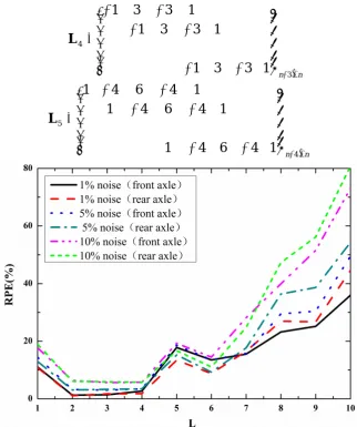
The abscissa values are corresponding to regularization matrices 𝐋𝐋₁ to 𝐋𝐋₁₀ in Fig.2,

respectively. The illustration results show the RPE values firstly decrease and then increase

with the increase of 𝑛𝑛-th derivative operators from identity matrix to ninth derivative

operators. By choosing proper regularization matrix 𝐋𝐋, such as the 𝐋𝐋₂, 𝐋𝐋₃and 𝐋𝐋₄, the RPE

values of PLSQR are much lower than LSQR without preconditioner and PLSQR with high

derivative operators from 𝐋𝐋₅ to 𝐋𝐋₁₀. When high derivative operators are adopted as

regularization matrix, the RPE values of PLSQR become higher than the those RPE values of

standard form LSQR method, which indicates that the identification accuracy of PLSQR

varies with different regularization matrices. The regularization matrix 𝐋𝐋 is a (𝑛𝑛 − 𝑝𝑝) ×𝑛𝑛

band matrix with full row rank where the number 𝑝𝑝 is corresponding to the 𝑝𝑝-th derivative

operator while the number 𝑝𝑝+ 1 is corresponding to the width of the band. As shown in the

following Eq. (20), the higher order the derivative operator is adopted, the larger the width of

the band is, which complicates the left and right orthogonal transformations due to less null

space of regularization matrix. Moreover, the resulting sparse problem with banded matrix

has effect on non-negative diagonal elements and efficacy of preconditioner. The fundamental

purpose of the preconditioner 𝐋𝐋+_𝐀𝐀(𝐋𝐋+_𝐀𝐀)𝑇𝑇 is to ensure the𝑗𝑗 iterative steps solution of PLSQR lies in the correct subspace and thus minimizes �𝐋𝐋𝐀𝐀_𝑗𝑗�

2. With high derivative operators from 𝐋𝐋5to𝐋𝐋10, the efficacy of preconditioner is reduced leading to large RPE values of PLSQR. The regularization matrices 𝐋𝐋₁,𝐋𝐋₂ , 𝐋𝐋₃,𝐋𝐋₄ and 𝐋𝐋₅are corresponding to LSQR, PLSQR(𝐋𝐋₂),

PLSQR(𝐋𝐋₃), PLSQR(𝐋𝐋₄) and PLSQR(𝐋𝐋₅), respectively, which can be shown as follow

n n×             = 1 1 1  1 L

(n−)×n             = 1 1 1 -1 1 -1 1 -  2 L

(n− )×n             − − − = 2 1 2 1 1 2 1 1 2 1    3

9

(n− )×n             − − − − − − = 3 4 1 3 3 1 1 3 3 1 1 3 3 1     L

(n− )×n             − − − − − − = 4 5 1 4 6 4 1 1 4 6 4 1 1 4 6 4 1      L

Fig.2. The RPE values identified by PLSQR with ten regularization matrices (1/2m&1/4a&1/2a)

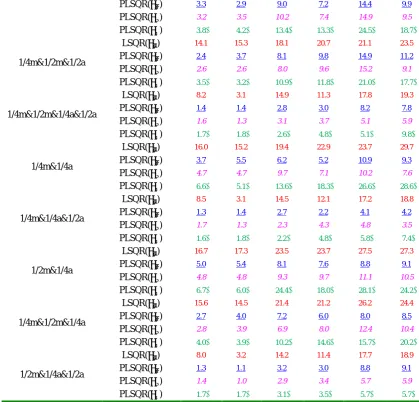
Table 1

The RPE values (%) identified by LSQR and PLSQR with three regularization matrices Sensor location regularization

matrix𝐋𝐋

1% noise 5% noise 10% noise front axle rear axle front axle rear axle front axle rear axle 1/4m&1/2m

LSQR(𝐋𝐋₁) 26.0 21.3 33.8 28.7 90.6 95.8

PLSQR(𝐋𝐋₂) 5.0 5.2 15.2 11.5 29.3 22.9

PLSQR(𝐋𝐋₃) 4.6 4.1 17.6 9.9 25.7 19.2

PLSQR(𝐋𝐋₄) （6.3） （4.6） （12.3） （9.1） （20.5） （16.4）

1/4m&1/2m&3/4m

LSQR(𝐋𝐋₁) 17.1 18.9 24.2 25.3 68.7 70.2

PLSQR(𝐋𝐋₂) 3.3 3.1 13.9 7.6 29.3 27.4

PLSQR(𝐋𝐋₃) 3.9 2.8 13.8 12.7 27.4 29.2

PLSQR(𝐋𝐋₄) （3.7） （2.8） （8.6） （6.9） （17.0） （12.0）

1/4a&1/2a

LSQR(𝐋𝐋₁) 7.4 3.2 13.3 10.3 16.8 16.4

PLSQR(𝐋𝐋₂) 0.5 1.2 2.8 2.9 5.4 5.6

PLSQR(𝐋𝐋₃) 1.4 0.9 2.4 2.7 4.3 4.7

PLSQR(𝐋𝐋₄) （1.7） （1.8） （3.4） （3.0） （4.9） （4.7）

1/4a&1/2a&3/4a

LSQR(𝐋𝐋₁) 0.6 1.1 2.5 5.2 4.4 11.8

PLSQR(𝐋𝐋₂) 0.5 1.1 1.9 1.4 2.8 3.1

PLSQR(𝐋𝐋₃) 0.7 0.9 1.5 2.5 2.7 3.9

PLSQR(𝐋𝐋₄) （1.7） （1.4） （1.7） （3.1） （2.8） （4.1）

10

PLSQR(𝐋𝐋₂) 3.3 2.9 9.0 7.2 14.4 9.9

PLSQR(𝐋𝐋₃) 3.2 3.5 10.2 7.4 14.9 9.5

PLSQR(𝐋𝐋₄) （3.8） （4.2） （13.4） （13.3） （24.5） （18.7）

1/4m&1/2m&1/2a

LSQR(𝐋𝐋₁) 14.1 15.3 18.1 20.7 21.1 23.5

PLSQR(𝐋𝐋₂) 2.4 3.7 8.1 9,8 14.9 11.2

PLSQR(𝐋𝐋₃) 2.6 2.6 8.0 9.6 15.2 9.1

PLSQR(𝐋𝐋₄) （3.5） （3.2） （10.9） （11.8） （21.0） （17.7）

1/4m&1/2m&1/4a&1/2a

LSQR(𝐋𝐋₁) 8.2 3.1 14.9 11.3 17.8 19.3

PLSQR(𝐋𝐋₂) 1.4 1.4 2.8 3.0 8.2 7.8

PLSQR(𝐋𝐋₃) 1.6 1.3 3.1 3.7 5.1 5.9

PLSQR(𝐋𝐋₄) （1.7） （1.8） （2.6） （4.8） （5.1） （9.8）

1/4m&1/4a

LSQR(𝐋𝐋₁) 16.0 15.2 19.4 22.9 23.7 29.7

PLSQR(𝐋𝐋₂) 3.7 5.5 6.2 5.2 10.9 9.3

PLSQR(𝐋𝐋₃) 4.7 4.7 9.7 7.1 10.2 7.6

PLSQR(𝐋𝐋₄) （6.6） （5.1） （13.6） （18.3） （26.6） （28.6）

1/4m&1/4a&1/2a

LSQR(𝐋𝐋₁) 8.5 3.1 14.5 12.1 17.2 18.8

PLSQR(𝐋𝐋₂) 1.3 1.4 2.7 2.2 4.1 4.2

PLSQR(𝐋𝐋₃) 1.7 1.3 2.3 4.3 4.8 3.5

PLSQR(𝐋𝐋₄) （1.6） （1.8） （2.2） （4.8） （5.8） （7.4）

1/2m&1/4a

LSQR(𝐋𝐋₁) 16.7 17.3 23.5 23.7 27.5 27.3

PLSQR(𝐋𝐋₂) 5.0 5.4 8.1 7.6 8.8 9.1

PLSQR(𝐋𝐋₃) 4.8 4.8 9.3 9.7 11.1 10.5

PLSQR(𝐋𝐋₄) （6.7） （6.0） （24.4） （18.0） （28.1） （24.2）

1/4m&1/2m&1/4a

LSQR(𝐋𝐋₁) 15.6 14.5 21.4 21.2 26.2 24.4

PLSQR(𝐋𝐋₂) 2.7 4.0 7.2 6.0 8.0 8.5

PLSQR(𝐋𝐋₃) 2.8 3.9 6.9 8.0 12.4 10.4

PLSQR(𝐋𝐋₄) （4.0） （3.9） （10.2） （14.6） （15.7） （20.2）

1/2m&1/4a&1/2a

LSQR(𝐋𝐋₁) 8.0 3.2 14.2 11.4 17.7 18.9

PLSQR(𝐋𝐋₂) 1.3 1.1 3.2 3.0 8.8 9.1

PLSQR(𝐋𝐋₃) 1.4 1.0 2.9 3.4 5.7 5.9

PLSQR(𝐋𝐋₄) （1.7） （1.7） （3.1） （3.5） （5.7） （5.7）

Note: Underlined RPE values are for PLSQR with bidiagonal matrix 𝐋𝐋₂, italics RPE values are for PLSQR with tri-diagonal matrix𝐋𝐋₃, the RPE values in parentheses are for PLSQR with four diagonal matrix 𝐋𝐋₄and other values are for LSQR withidentity matrix 𝐋𝐋₁.

Table 1 tabulates the RPE values of LSQR and PLSQR with three different regularization

matrices in 12 cases. When LSQR is adopted to identify the biaxial time-varying forces, the

RPE values are less than 30% in 10 cases out of all 12 cases with 1%, 5% and 10% noise levels. Jacobsen and Hansen [35] pointed out that the regularization method is a good means

of solving ill-posed problem. Preconditioned LSQR is a typical regularization approach by

choosing proper regularization matrix to solve or to reduce the effects of ill-posedness on

identification results.

When PLSQR(𝐋𝐋2), PLSQR(𝐋𝐋3) and PLSQR(𝐋𝐋4) are adopted to identify the biaxial

time-varying forces, the RPE values are less than 30% in all 12 cases with three kinds of noise

levels. Moreover, with the noise level increases, the RPE values of PLSQR only increase

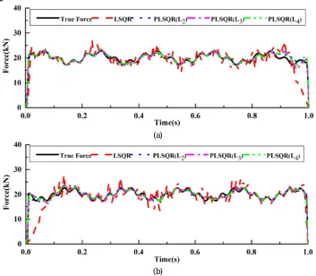
slightly owing to its strong robustness. As shown in the Fig.3 to Fig.5, the identification

forces of PLSQR are very close to the true forces under various cases due to good adaptability

11

PLSQR is much better than LSQR when both front and rear axles are not simultaneously

present on the beam, which means that the PLSQR has strong immunity of ill-posed problem.

Considering altogether the RPE values of PLSQR(𝐋𝐋₂), PLSQR(𝐋𝐋₃) and PLSQR(𝐋𝐋₄) in all

12 cases, the RPE values of PLSQR(𝐋𝐋₃) are relatively smaller than PLSQR(𝐋𝐋₂) and

PLSQR(𝐋𝐋₄). Simultaneously, the matrix 𝐋𝐋₃ is chosen as regularization matrix of PLSQR

firstly, and then the calibration studies are carried out with static force, single axle force and

other biaxial time-varying forces. All of the results show that the matrix 𝐋𝐋₃of PLSQR has

high identification accuracy and can be chosen as regularization matrix of PLSQR in MFI,

which is case independent. Then the matrix 𝐋𝐋₃ is chosen as the optimal regularization matrix

of PLSQR and will be default adopted in subsequent studies. As mentioned above, the

PLSQR is a hybrid method between a direct and an iterative regularization algorithm and the

identification accuracy of PLSQR is influenced by the number of iterations. The optimal

number of iterations is adopted in this study and will be examined in details in the next

section.

(a)

(b)

12 (a)

(b)

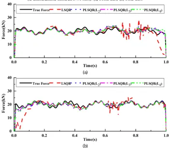
Fig.4. MFI from combined responses by LSQR and PLSQR with three regularization matrices (1/4m&1/2m&1/4a&1/2a 5% Noise). (a) Front axle; (b) Rear axle.

(a)

(b)

Fig.5. MFI from combined responses by LSQR and PLSQR with three regularization matrices (1/2m&1/4a&1/2a 10% Noise). (a) Front axle; (b) Rear axle.

13

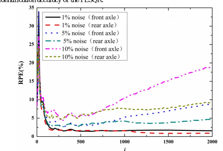
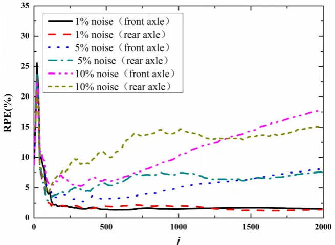
As shown in the Fig.6, the RPE values of MFI from acceleration responses maintain less

than 3% from 200 to 2000 with 1% noise level. It means that when the noise level is low it is

not necessary to find optimal number of iteration because the calculation time and the

identification cost outweigh the benefit. The efficacy of the optimal number of iterations

when there is a high level of noise will be investigated further in this section. As shown in

Table 2, the optimal number of iterations 𝑗𝑗3 is determined by RPE values compared

identification force with true force. So there is obvious limitationwithout knowing the actual

moving force. As shown in the Fig.6 to Fig.8, the effect of the number of iterations has

similar behavior when acceleration responses contained in MFI. With increasing the number

of iterations, the RPE values firstly increase rapidly and then decrease sharply, and then the

RPE values keep asmall fluctuation in the middle of the curve. When the number of iterations is selected close to 200, the RPE values are quite low in all cases as shown in the Fig.6 to

Fig.9. The normal number of iterations 𝑗𝑗4 = 200 is therefore selected to compare with other

number of iterations in the following studies.

As shown in the Fig.6 to Fig.8, the RPE values curve has a significant peak corresponding

to abscissa values 20 and then the worst number of iterations 𝑗𝑗2 = 20 is selected to reveal the

reasons. At the same time, the RPE values are still relatively small corresponding to very

small abscissa values and then the minimum number of iterations 𝑗𝑗1 = 1 is selected to reveal

the identification results of the PLSQR(𝐋𝐋₃) with number of iterations only once.

As shown in the Fig.9, when moving force is identified from bending moment responses

alone, the RPE values will exceed 100% when the number of iterations exceeds 1000 with 10%

noise level. Therefore, choosing the optimal number of iterations has significant influence on

the identification accuracy of the PLSQR.

14

Fig.7. The RPE values of different number of iterations 𝑗𝑗 in MFI by PLSQR from three combined responses (1/2m&1/4a&1/2a)

15

Fig.9. The RPE values of different number of iterations 𝑗𝑗 in MFI by PLSQR from three bending moment responses (1/4m&1/2m&3/4m)

Table 2 tabulates the RPE values of PLSQR(𝐋𝐋₃) with four different numbers of iterations in

all 12 cases. The results show that the RPE values are less than 30% in all 12 cases and almost

remain constant with noise level increasing when the minimum number of iterations 𝑗𝑗1 = 1 is

selected. While as shown in the Fig.10 to Fig.12,the identification results are similar to the

average load and cannot truly reflect the load fluctuations with number of iterations 𝑗𝑗1 = 1.

As shown in Fig.10 to Fig.12, the RPE values of PLSQR(𝐋𝐋₃) become largest with number

of iterations 𝑗𝑗2 = 20 due to the ill-posed problem, especially when both front and rear axles

are not simultaneously present on the beam. Consequently, it is suggested that the number of 𝑗𝑗2 = 20 should be excluded in PLSQR(𝐋𝐋₃).

When the optimal number of iterations 𝑗𝑗3 and the reasonable number of iterations 𝑗𝑗4 =

200 selected, both of the identification forces of the two kinds of number of iterations are very close to the true forces as shown in Table 2 and Fig.10 to Fig.12. It means that when the

optimal number of iterations cannot be reasonably determined without knowing the actual

moving force, the normal number of iterations𝑗𝑗4 = 200 of PLSQR(𝐋𝐋₃) can be selected to

facilitate MFI.

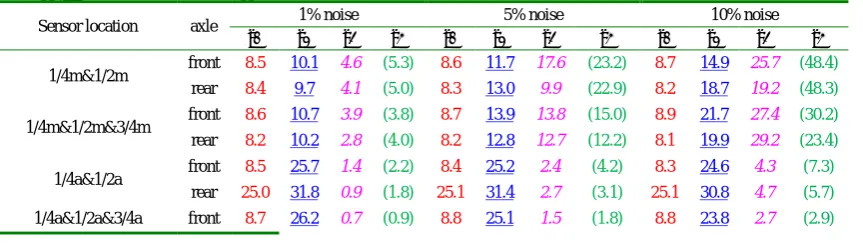
Table 2

The RPE values (%) of PLSQR(𝐋𝐋₃) with four different numbers of iterations

Sensor location axle 1% noise 5% noise 10% noise

𝑗𝑗1 𝑗𝑗2 𝑗𝑗3 𝑗𝑗4 𝑗𝑗1 𝑗𝑗2 𝑗𝑗3 𝑗𝑗4 𝑗𝑗1 𝑗𝑗2 𝑗𝑗3 𝑗𝑗4

1/4m&1/2m front 8.5 10.1 4.6 (5.3) 8.6 11.7 17.6 (23.2) 8.7 14.9 25.7 (48.4) rear 8.4 9.7 4.1 (5.0) 8.3 13.0 9.9 (22.9) 8.2 18.7 19.2 (48.3)

1/4m&1/2m&3/4m front 8.6 10.7 3.9 (3.8) 8.7 13.9 13.8 (15.0) 8.9 21.7 27.4 (30.2) rear 8.2 10.2 2.8 (4.0) 8.2 12.8 12.7 (12.2) 8.1 19.9 29.2 (23.4)

1/4a&1/2a front 8.5 25.7 1.4 (2.2) 8.4 25.2 2.4 (4.2) 8.3 24.6 4.3 (7.3) rear 25.0 31.8 0.9 (1.8) 25.1 31.4 2.7 (3.1) 25.1 30.8 4.7 (5.7)

16

rear 26.8 25.9 0.9 (1.8) 26.8 25.4 2.5 (2.6) 26.9 24.9 3.9 (4.4)

1/2m&1/2a front 9.0 29.9 3.2 (3.4) 8.9 33.7 10.2 (10.5) 8.7 35.0 14.9 (21.4) rear 13.4 30.9 3.5 (3.6) 13.1 30.0 7.4 (10.8) 12.8 30.7 9.5 (21.5)

1/4m&1/2m&1/2a front 8.7 30.2 2.6 (3.5) 8.7 30.4 8.0 (8.2) 8.6 30.8 15.2 (16.5) rear 12.1 29.5 2.6 (3.0) 12.0 29.3 9.6 (11.4) 11.9 31.0 9.1 (23.5)

1/4m&1/2m&1/4a&1/2a front 8.9 23.0 1.6 (1.9) 8.8 22.3 3.1 (3.7) 8.7 21.6 5.1 (6.7) rear 15.1 24.7 1.3 (2.1) 14.9 24.3 3.7 (4.2) 14.8 24.0 5.9 (7.9)

1/4m&1/4a front 9.1 24.9 4.7 (9.4) 9.0 23.0 9.7 (18.4) 8.9 20.8 10.2 (33.7) rear 17.8 24.2 4.7 (5.9) 17.9 23.7 7.1 (14.3) 18.1 23.1 7.6 (27.0)

1/4m&1/4a&1/2a front 9.1 26.9 1.7 (1.9) 9.1 26.5 2.3 (3.2) 9.0 26.1 4.8 (5.8) rear 19.0 27.1 1.3 (2.1) 19.0 26.7 4.3 (4.2) 19.1 26.2 3.5 (8.1)

1/2m&1/4a front 9.0 31.4 4.8 (8.2) 8.8 29.0 9.3 (17.0) 8.6 26.4 11.1 (34.3) rear 14.8 26.6 4.8 (6.1) 14.5 25.0 9.7 (14.6) 14.1 23.2 10.5 (29.6)

1/4m&1/2m&1/4a front 8.8 25.8 2.8 (7.4) 8.7 25.4 6.9 (7.0) 8.7 25.4 12.4 (13.2) rear 13.2 23.5 3.9 (4.0) 13.0 24.3 8.0 (8.2) 12.8 25.7 10.4 (17.2)

1/2m&1/4a&1/2a front 9.1 24.7 1.4 (1.9) 9.0 24.0 2.9 (4.3) 8.8 23.2 5.7 (8.0) rear 16.7 27.8 1.0 (2.0) 16.4 27.1 3.4 (3.3) 16.2 26.1 5.9 (6.2)

Note: Underlined RPE values are for PLSQR(𝐋𝐋₃) with the worst number of iterations 𝑗𝑗2 = 20, italics RPE values are for PLSQR(𝐋𝐋₃) with the optimal number of iterations 𝑗𝑗3, the RPE values in parentheses are for PLSQR(𝐋𝐋₃) with normal number of iterations 𝑗𝑗4 = 200and other RPE values are for PLSQR(𝐋𝐋₃) with the minimum number of iterations 𝑗𝑗1 = 1.

(a)

(b)

17 (a)

(b)

Fig.11. MFI from combined responses by PLSQR with four different numbers of iterations𝑗𝑗 (1/4m&1/2m&1/2a 5% Noise). (a) Front axle; (b) Rear axle.

(a)

(b)

Fig.12. MFI from acceleration responses by PLSQR with four different numbers of iterations𝑗𝑗 (1/4a&1/2a 10% Noise). (a) Front axle; (b) Rear axle.

18

Former part of this study shows that all of the PLSQR(𝐋𝐋₂), PLSQR(𝐋𝐋₃) and PLSQR(𝐋𝐋₄)

have strong robustness to responses noise and ill-posedness problem. Then the identification

ability of PLSQR will be compared with the TDM in this part. The illustration results of

Fig.13 show that MFI from bending moment responses alone by TDM suffers from large

fluctuation even with only one percent noise level added. When combined responses from

two sensors are used, the accuracy of TDM is also unacceptable as shown in Fig.14. Only

when three acceleration responses used alone, the identification accuracy of TDM is

improved being similar to that of PLSQR as shown in Fig.15. It means that the TDM is

sensitive to both the type of sensors and the number of sensors; the identification results will

unacceptable when bending moment measurements are used alone or the number of sensors is

small.

Comparing with TDM, the biaxial moving forces identified by PLSQR(𝐋𝐋₂), PLSQR(𝐋𝐋₃)

and PLSQR(𝐋𝐋₄) are very close to the true forces in all cases as shown in Fig.13 to Fig.15. The

PLSQR has excellent adaptability with both the type of sensors and the number of sensors.

The numerical simulation results also show that the accuracy and acceptability of

identification forces by PLSQR will improve with more acceleration responses and lower

disturbance noise. In order to facilitate the economical application of the PLSQR in field tests,

specific sensor requirements are suggested as follows. When noise level is less than 5%, at

least two responses are measured and at least one acceleration response is included. When

noise level is higher than 5%, at least three responses are measured and at least two

acceleration responses are included.

As the moving speed is an important factor affecting in MFI, the effect of the moving

speed on PLSQR(𝐋𝐋₃) is simulated with three decreasing moving speeds, namely 𝑐𝑐₁= 40m∙

s−1_{, 𝑐𝑐}

2 = 30m∙s−1 and 𝑐𝑐3= 20m∙s−1, respectively. The time for passing over the bridge corresponding to these three speeds is 1s, 4

3s and 2s, respectively. Due to the consistency rule of the effect of vehicle speed on PLSQR(𝐋𝐋₃), Table 3 tabulates four representative cases from

all 12 cases. The simulation results show that the identification accuracy is slightly improved

and the optimal number of iterations is increased with the decrease of the speed. Similar to

the normal number of iterations 𝑗𝑗4 = 200 of PLSQR(𝐋𝐋₃) can be selected to facilitate MFI

with speed 𝑐𝑐₁, the normal number of iterations 𝑗𝑗= 220 and 𝑗𝑗= 300 can be selected to

facilitate MFI corresponding to speed 𝑐𝑐₂ and speed 𝑐𝑐₃, respectively.

As shown in Fig.16 and Fig.17, the biaxial moving forces identified by PLSQR(𝐋𝐋₃) are

very close to the true forces during the vehicle crosses the bridge with all three speeds. The

illustration results show that the identification accuracy of PLSQR remains at a high level

with different moving speeds, which is very beneficial for the application of PLSQR method

19 (a)

(b)

Fig.13. MFI by PLSQR and TDM from two bending moment responses (1/4m&1/2m 1% Noise). (a) Front axle; (b) Rear axle.

(a)

(b)

20 (a)

(b)

Fig.15. MFI by PLSQR and TDM from three acceleration responses (1/4a&1/2a&3/4a 10% Noise). (a) Front axle; (b) Rear axle.

Table 3

The RPE values (%) of PLSQR(𝐋𝐋₃) with three different moving speeds

Sensor location axle 1% noise 5% noise 10% noise

𝑐𝑐1 𝑐𝑐2 𝑐𝑐3 𝑐𝑐1 𝑐𝑐2 𝑐𝑐3 𝑐𝑐1 𝑐𝑐2 𝑐𝑐3

1/4m&1/2m&3/4m front 3.9 2.7 2.7 13.8 9.3 7.3 27.4 23.3 19.9 rear 2.8 3.2 2.7 12.7 10.6 6.8 29.2 29.0 20.8

1/4m&1/2m&1/4a&1/2a front 1.6 1.6 1.5 3.1 2.7 2.6 5.1 4.1 4.1 rear 1.3 1.3 1.3 3.7 3.3 2.2 5.9 5.2 3.1

1/4m&1/4a&1/2a front 1.7 1.6 1.5 2.3 2.7 2.7 4.8 4.2 4.0 rear 1.3 1.3 1.3 4.3 2.7 2.4 3.5 3.7 3.0

1/2m&1/4a&1/2a front 1.4 1.4 1.3 2.9 3.0 3.0 5.7 4.4 4.3 rear 1.0 1.0 1.0 3.4 3.2 2.4 5.9 4.8 3.4

Note: Italics RPE values are for PLSQR(𝐋𝐋₃) with the moving speed 𝑐𝑐₁= 40m∙s−1, underlined RPE values are for PLSQR(𝐋𝐋₃) with the moving speed 𝑐𝑐₂= 30m∙s−1 and other RPE values are for PLSQR(𝐋𝐋₃) with the moving speed 𝑐𝑐₃= 20m∙s−1.

21 (b)

Fig.16. MFI with three different speeds by PLSQR(𝐋𝐋₃) from acceleration responses (1/4m&1/2m 1% Noise). (a) Front axle; (b) Rear axle.

(a)

(b)

Fig.17. MFI with three different speeds by PLSQR(𝐋𝐋₃) from acceleration responses (1/4a&1/2a&3/4a 10% Noise). (a) Front axle; (b) Rear axle.

4. Conclusions

In this work, a PLSQR method is proposed to identify moving force by preconditioning

LSQR. By means of numerical simulations, a comprehensive parametric study has been done

and the following conclusions can be drawn:

(1) When PLSQR(𝐋𝐋2), PLSQR(𝐋𝐋3) and PLSQR(𝐋𝐋4) are adopted to identify the moving

force, the identification accuracy in all 12 cases is significantly improved compared with

LSQR(𝐋𝐋1 ). The PLSQR has overcome the ill-posed problem by choosing proper

22

PLSQR(𝐋𝐋₂) and PLSQR(𝐋𝐋₄) as mentioned above. Then the matrix 𝐋𝐋₃ is selected as the

optimal regularization matrix for preconditioning LSQR.

(2) When the optimal number of iterations 𝑗𝑗3 and the reasonable number of iterations 𝑗𝑗4 =

200 selected, both of the identification forces of the two kinds of number of iterations are very close to the true forces as shown previously. It means that when the optimal number of

iterations cannot be determined without knowing the actual moving force, the normal number

of iterations 𝑗𝑗4 = 200 of PLSQR(𝐋𝐋₃) can be selected which also meet the requirements of

MFI. On the contrary, the number of iterations 𝑗𝑗1 = 1 and 𝑗𝑗2 = 20 of PLSQR(𝐋𝐋₃) should be

avoided as the former cannot truly reflect the load fluctuations and the latter amplify the

ill-posed problem.

(3) Comparing with TDM, the identification accuracy of PLSQR is much higher in all

cases. The PLSQR has excellent adaptability with both the type of sensors and the number of

sensors, it also has strong noise immunity and robust with ill-posed problem. Moreover, the

identification accuracy is slightly improved with the decrease of the speed. The illustrated

results show that the identification accuracy of PLSQR(𝐋𝐋₃) remains at a very high level with

different moving speeds, which highlights the robustness of PLSQR method infield tests.

Finally, it is noted that,compared with the situations that both of the axles are running on

the bridge, the identification accuracy of PLSQR is still lower when only either the front or

rear axle is on the bridge. It is therefore suggested that MFI through PLSQR not be performed

during these situations, and this problem will be investigated further in future works of the

present authors. In addition, further studies about the independent of regularization matrix

selecting and the improvement of identification efficiency without sacrificing the

identification accuracy will also be discussed in the next paper.

Acknowledgments

This research was supported by Key Science and Technology Program of Henan Province,

China (Grant Number 192102310011), MOE Key Lab of Disaster Forecast and Control in

Engineering, Jinan University (Grant Number 20180930003) and National Natural Science

Foundation of China (Grant Numbers 51678278 and 51278226).

References:

[1] M. Lydon, S.E. Taylor, D. Robinson, A. Mufti, E.J.O. Brien. Recent developments in bridge weigh in motion (B-WIM), J. Civil Struct. Health Monit. 6 (2016) 69-81.

[2] J. Sanchez, H. Benaroya, Review of force reconstruction techniques, J. Sound Vib. 333 (2014) 2999-3018. [3] C. O’Connor, T.H.T. Chan, Dynamic wheel loads from bridge strains, Eng. Struct. 114 (1988) 1703-1723. [4] S.S. Law, T.H.T. Chan, Q.H. Zeng, Moving force identification: a time domain method, J. Sound Vib. 201(1)

(1997) l-22.

[5] T.H.T. Chan, S.S. Law, T.H. Yung, X.R. Yuan, An interpretive method for moving force identification, J. Sound Vib. 219 (1999) 503-524.

[6] S.S. Law, T.H.T. Chan, Q.H. Zeng, Moving force identification-a frequency and time domains analysis, J. Dyn. Sys. Meas. Control ASME 121 (1999) 394-401.

23

[8] X.Q. Zhu, S.S. Law, Identification of vehicle axle loads from bridge dynamic responses, J. Sound Vib. 236 (2000) 705-724.

[9] X.Q. Zhu, S.S. Law, Identification of moving interaction forces with incomplete velocity information, Mech. Syst. Signal Process. 17 (2003) 1349-1366.

[10] X.Q. Zhu, S.S. Law, Moving load identification on multi-span continuous bridges with elastic bearings, Mech. Syst. Signal Process. 20 (2006) 1759-1782.

[11] T.H.T. Chan, D.B. Ashebo, Theoretical study of moving force identification on continuous bridges, J. Sound Vib. 295 (2006) 870-883.

[12] L. Yu, T.H.T. Chan, J.H. Zhu, A MOM-based algorithm for moving force identification: Part I - Theory and numerical simulation, Struct. Eng. Mech. 29 (2008) 135-154.

[13] Y. Yu, C.S. Cai, L. Deng, State-of-the-art review on bridge weigh-in-motion technology, Adv. Struct. Eng. 19 (2016) 1514-1530.

[14] J. Dowling, E.J. Obrien, A. González, Adaptation of cross entropy optimization to a dynamic bridge WIM calibration problem, Eng. Struct. 44 (2012) 13-22.

[15] A. Berry, O. Robin, F. Pierron, Identification of dynamic loading on a bending plate using the virtual fields method, J. Sound Vib. 333 (2014) 7151-7164.

[16] Z. Li, Z.P. Feng, F.L. Chu, A load identification method based on wavelet multi-resolution analysis, J. Sound Vib. 333 (2014) 381-391.

[17] T. Pinkaew, Identification of vehicle axle loads from bridge responses using updated static component technique, Eng. Struct. 28 (2006) 1599-1608.

[18] A. González, C. Rowley, E.J. Obrien, A general solution to the identification of moving vehicle forces on a bridge, Int. J. Numer. Methods Eng. 75 (2008) 335-354.

[19] Y.M. Mao, X.L. Guo, Y. Zhao, A state space force identification method based on Markov parameters precise computation and regularization technique, J. Sound Vib. 329 (2010) 3008-3019.

[20] H. Ronasi, H. Johansson, F. Larsson, A numerical framework for load identification and regularization with application to rolling disc problem, Comput. Struct. 89 (2011) 38-47.

[21] S.Q. Wu, S.S. Law, Moving force identification based on stochastic finite element model, Eng. Struct. 32 (2010) 1016-1027.

[22] Y. Ding, S.S. Law, Structural damping identification based on an iterative regularization method, J. Sound Vib. 330 (2011) 2281-2298.

[23] J. Li, S.S. Law, H. Hao, Improved damage identification in bridge structures subject to moving loads: numerical and experimental studies, Int. J. Mech. Sci. 74 (2013) 99-111.

[24] Y. Ding, S.S. Law, B. Wu, G.S. Xu, Q. Lin, H.B. Jiang, Q.S. Miao, Average acceleration discrete algorithm for force identification in state space, Eng. Struct. 56 (2013) 1880-1892.

[25] D.M. Feng, H. Sun, M.Q. Feng, Simultaneous identification of bridge structural parameters and vehicle loads, Comput. Struct. 157 (2015) 76-88.

[26] B.J. Qiao, X.F.Chen, X.F.Xue, X.J.Luo, R.N.Liu, The application of cubic B-spline collocation method in impact force identification, Mech. Syst. Signal Process. 64-65 (2015) 413-427.

[27] B.J. Qiao, X.W. Zhang, X.J. Luo, X.F. Chen, A Force identification method using cubic b-spline scaling functions, J. Sound Vib. 337 (2015) 28-44.

[28] J. Liu, X.S. Sun, X. Han, A novel computational inverse technique for load identification using the shape function method of moving least square fitting, Comput. Struct. 144 (2014) 127-137.

[29] X.S. Sun, J. Liu, X. Han, A new improved regularization method for load identification, Inverse Probl. Sci. Eng. 22(2014) 1602-1076.

[30] J. Liu, X.S. Sun, X. Han, Dynamic load identification for stochastic structures based on Gegenbauer polynomial approximation and regularization method, Mech. Syst. Signal Process. 56-57 (2015) 35-54. [31] J. Liu, X.H. Meng, C. Jiang, X. Han, D.Q. Zhang, Time-domain Galerkin method for dynamic load

identification,Int. J. Numer. Methods Eng. 105 (2016) 620-640.

[32] C.C. Paige, M.A. Saunders, LSQR: An algorithm for sparse linear equations and sparse least squares, ACM T. Math. Software 8 (1982) 43-71.

[33] M.A. Saunders, Solution of sparse rectangular systems using LSQR and CRAIG, BIT Numer. Math. 35 (1995) 588-604.

[34] S.J. Benbow, Solving generalized least-squares problems with LSQR, SIAM J. Matrix Anal. Appl. 21 (1999) 166-177.

[35] M. Jacobsen, P.C. Hansen, M.A. Saunders, Subspace preconditioned LSQR for discrete ill-posed problems, BIT Numer. Math. 43 (2003) 975-989.

[36] L. Reichel, Q. Ye, A generalized LSQR algorithm, Numer. Linear Algebra Appl. 15 (2008) 643-660. [37] J. Baglama, L. Reichel, D. Richmond, An augmented LSQR method, Numer. Algorithms 64 (2013) 263-293. [38] S. Karimi, B. Zali, The block preconditioned LSQR and GL-LSQR algorithms for the block partitioned

matrices, Appl. Math. Comput. 227 (2014) 811-820.