Holomorphic anomaly equations in topological string theory

String Theory

Thesis by

Jie Yang

In Partial Fulfillment of the Requirements for the Degree of

Doctor of Philosophy

California Institute of Technology Pasadena, California

2008

c

2008

Acknowledgments

I am deeply grateful to my advisor, Hirosi Ooguri. His patience, encouragement, support and wisdom have been guiding me through my Ph.D. study. His insightful ideas and enthusiasm in string theory inspire me in this field. I am greatly thankful for his generous help in working out the projects. This thesis would not be possible without his kind efforts.

I thank Mark Wise for giving me a good opportunity to work as his teaching assistant. I have learned lot of physics as well as teaching from him. I also thank him for serving on my defense committee.

I thank Anton Kapustin for teaching me physics and mathematics as well as serving on my defense and candidacy committees.

I thank John Schwarz for teaching me supersymmetry and string theory and for serving on my candidacy committee.

I thank Frank Porter for teaching me high energy physics. As a string theory student, it is the highest experiment to theory ratio course that I have taken. I also thank him for serving on my defense committee.

I thank Alan Weinstein for serving on my candidacy committee.

I thank Sergei Gukov for teaching me topological field theory and giving me a chance to present in his class.

I thank Marc Kamionkowski for teaching me QHE and BCS theory, and I thank Chris Hirata for teaching me standard cosmology. From them I obtained great help in preparing solutions to homework.

advice in research. Lotty Ackerman is the friend who always gives me a big hug, which makes me smile all day. Jaewon Song shares with me a lot of his understanding about meta-stable vacua and inflation. Tudor Dimofte is a friend who has great talent in both string theory and the violin, I am happy to have memories of his wonderful performances. Donal O’Connell, Yi Li, and Tukuya Okuda are the best teaching assistants that I have met. Sonny Mantry helped me to use CTEQ in calculating Higgs production.

I am honored to have support and friendship from Joe Marsano, Matt John-son, Chang Soon Park, Yutaka Ookouchi, Natalia Saulina, Andrei Mikhailov, Kirill Saraikin, Kevin Setter, Miguel Bandres, Arthur Lipstein, Masaki Shigemori, Andrew Frey, Alejandro Jenkins, Ian Swanson, and Tristan McLoughlin.

I thank Carol Silberstein for being a kind-hearted friend who cares about me and helps me with lots of things. She is also a friend from whom I learned a lot of American culture. I thank Kovid Goyal for generous help with my computer.

I owe a lot to my best friend Fangwei Shao. She is someone I trust a lot and to whom I turn for help immediately when I encounter a problem. I owe a lot to my good friends and my apartmentmates Hsin-Ying Chiu and Shih-Jung Huang for taking care of me in my daily life. I thank Hsin-Ying for explaining to me nano physics. It is my fortune to have the friendship and blessing from Jing Yang, Ke Wang, Jiang Xia, Rong Cai, Yanshun Liu, Minnie He, Kuan Li, Cindy Fan, Charlie Zhu, He He, Zhiying Song, Jup H. Wen, Yih C. Wen, Amanda Ho, Ying-Chin Ku, Kang Hu, Icy Ma, Yongqin Jiao, and Jiansong Gao.

Abstract

In this thesis we discuss various aspects of topological string theories. In particular we provide a derivation of the holomorphic anomaly equation for open strings and study aspects of the Ooguri, Strominger, and Vafa conjecture.

Topological string theory is a computable theory. The amplitudes of the closed topological string satisfy a holomorphic anomaly equation, which is a recursive dif-ferential equation. Recently this equation has been extended to the open topological string. We discuss the derivation of this open holomorphic anomaly equation. We find that open topological string amplitudes have new anomalies that spoil the recur-sive structure of the equation and introduce dependence on wrong moduli (such as complex structure moduli in the A-model), unless the disk one-point functions vanish. We also show that a general solution to the extended holomorphic anomaly equation for the open topological string on D-branes in a Calabi-Yau manifold, is obtained from the general solution to the holomorphic anomaly equations for the closed topo-logical string on the same manifold, by shifting the closed string moduli by amounts proportional to the ’t Hooft coupling.

Contents

Acknowledgments iii

Abstract v

1 Introduction 1

2 Topological String Theory 4

2.1 Introduction . . . 4

2.2 N = (2,2) supersymmetry . . . 5

2.3 Topological sigma model . . . 7

2.3.1 U(1)R anomaly . . . 9

2.4 Closed topological string theory . . . 10

2.4.1 Bosonic string theory . . . 11

2.4.2 Closed topological string amplitudes . . . 12

2.4.3 Relation between closed topological strings and physical strings 13 3 The Open Holomorphic Anomaly Equation 14 3.1 Introduction . . . 14

3.2 The open topological string theory . . . 16

3.2.1 Boundary condition . . . 16

3.2.2 Some aspects of the moduli spaces of Riemann surfaces . . . . 16

3.2.3 Open holomorphic anomaly equation . . . 19

3.3 New anomalies in topological string theory . . . 20

3.3.1 Physical meaning of the new anomalies . . . 20

3.3.2 Anomalous worldsheet degenerations . . . 21

3.4 Small number of moduli . . . 28

3.4.2 Some discussion . . . 32

3.5 Feynman rules to solve the holomorphic anomaly equation . . . 33

4 The Relation between the Open and Closed Topological String 36 4.1 Generating function . . . 36

4.2 The closed string moduli and coupling . . . 39

5 Applying the Ooguri, Strominger, and Vafa Conjecture 42 5.1 Introduction . . . 42

5.2 OSV conjecture . . . 43

5.3 Small black hole . . . 46

5.4 Second approach to handling non-perturbative corrections . . . 51

5.5 Gromov-Witten invariants . . . 52

5.6 Modularity and holomorphicity . . . 57

6 Summary and Open Questions 66 A Explicit Extrapolation Formulae 69 A.1 Low genus/boundary topological string holomorphic equation . . . . 69

A.2 New approach to factorize Yang-Mills partition function . . . 73

A.2.1 Topological string side . . . 73

A.2.2 Yang-Mills side . . . 74

A.3 (Almost) modular forms . . . 77

List of Figures

3.1 A handle pinches off . . . 18

3.2 An equator pinches off . . . 18

3.3 A strip pinches off and results in two Riemann surfaces . . . 18

3.4 A strip pinches off and removes a handle . . . 18

3.5 Two boundaries join up and result in one boundary . . . 18

3.6 A boundary shrinks . . . 18

3.7 Tadpole . . . 20

3.8 Disk one-point function . . . 20

3.9 yp _{derivative with insertion near a boundary . . . . 27}

3.10 yp _{derivative with insertion away from a boundary . . . . 27}

3.11 ¯t¯i _{derivative with insertion away from a boundary . . . . 27}

3.12 Cylinder . . . 29

3.13 Blow up of the colliding of two operators . . . 30

3.14 Boundary colliding . . . 30

3.15 Disk two-point functions . . . 31

3.16 Disk one-point function . . . 32

3.17 The propagators for Feynman diagrams of topological string amplitudes 34 3.18 Feynman diagrams for F(2,0) _{. . . . 35}

3.19 Feynman diagrams for F(1,1) _{. . . . 35}

5.1 Fermion system vs Young diagram . . . 48

5.2 Chiral factorization . . . 49

5.3 Free fermion realized large N factorization . . . 50

5.4 New resummation laws . . . 51

5.5 New partition function . . . 52

List of Tables

2.1 U(1) charges of fermionic fields under A- and B-twist . . . 8

2.2 Cohomological structures under A- and B-twist . . . 8

2.3 Bosonic string vs A-model topological string . . . 11

Chapter 1

Introduction

String theory is a candidate theory that unifies all four forces of nature. As a fun-damental theory, it has great beauty. This theory has constituents that are tiny 1-dimensional objects called strings. Their typical scale is thought to be about 10−35_m

which in terms of energy is about 1019_{GeV, the Planck scale. It is therefore hard}

to do any direct observation of strings, since the highest energy scale experimentally accessible today is 14 TeV at the Large Hadron Collider (LHC). We can perhaps obtain cosmological evidence, but even the Big Bang does not seem to provide high-enough energies. Another way to test string theory is to investigate its low energy behavior and compare with experiments. String theory requires spacetime to have a critical dimension. Superstring theory gives a spacetime dimension of 10. This raises questions about how to compactify this theory on a particular manifold, so that when the size of this manifold is very small it gives us 4-dimensional physics as we observe it. Unfortunately, compactification is not so simple and causes many problems.

In particular we care about a 4-dimensional low-energy effective theory of super-string theory compactified on certain manifolds. The manifold we consider through-out this thesis is a 3-complex or 6-real dimensional Calabi-Yau manifold, termed a Calabi-Yau 3-fold, which reduces supersymmetries to a quarter in d= 4.

string theory. Furthermore the topological string theory in a Calabi-Yau 3-fold has the same structure as a bosonic string theory. This theory became more important when its physical application was discovered.

Closed topological string theory is well-understood [1, 2]. Topological string theory with D-branes, i.e., open strings, is also interesting, because these carry gauge degrees of freedom. In particular we hope it will help us to understand open-closed dualities in string theory. These dualities originate in the so called holographic principle— gauge/geometry correspondence. It was found that Chern-Simons gauge theory on a 3-dimensional manifold M can be viewed as a topological string theory on T∗_M [3]. The argument is that the perturbative expansion of this string theory coincides with Chern-Simons perturbation theory. Later, it was found that the large N limit of SU(N) Chern-Simons theory on S3 _{is the same as an N = 2 topological closed}

string on the S2 _{blowup of the conifold geometry inT}∗_S3_{. There also exists an open}

topological string description of the duality whereN 3-branes are wrapped on anS3

inside the conifold T∗_S3 _{[4]. Furthermore, [5, 6] gave a worldsheet explanation of the}

duality between open and closed topological strings.

B-model depends on K¨ahler moduli.

We also derived a generating function for amplitudes of the open topological string on D-branes in a Calabi-Yau manifold. Interestingly, it is related to the generating function of the closed topological string on the same manifold [1], by shifting the closed string moduli by amounts proportional to the ’t Hooft coupling [9].

One important application of the closed topological string theory is the Ooguri, Strominger, and Vafa (OSV) conjecture. It says that, in the large black hole limit where the black hole was obtained by type II superstring compactified on a Calabi-Yau 3-fold, the black hole partition function is the absolute value of square of a topo-logical string partition function. For small black holes, there are non-perturbative corrections, for example in the factorization of two baby universes, there will be contributions from 2n (n > 2) baby universes [10]. We attempted to build a new factorization and tried to interpret it as a “non-perturbative” completion of the topo-logical string partition function. In order to prove that, it is necessary to check if it satisfies holomorphic anomaly equation. For topological string theory, holomor-phicity and modularity can be shown to be traded with each other. The partition functions of baby universes are already written in a holomorphic form but they are not modular. We thus want to understand how we can restore the modular property and then obtain the holomorphic anomaly equation.

Chapter 2

Topological String Theory

2.1

Introduction

There are various formulations of superstring theory. The worldsheet, for example, can be described by an N = 1 supersymmetric Ramond-Neveu-Schwarz (RNS) for-malism or a spacetime Green-Schwarz (GS) forfor-malism. However calculating string scattering, the most important physical process in a quantum theory of strings, is very difficult in both formalisms. The physical string theory must have excitations that correspond to every kind of elementary particle. Bosonic string theory does not provide a description of fermions, but fermion fields can be added to the action by considering superstring theory. It was found when string worldsheet supersymmetry is extended toN = 2, some nice geometrical feature appears which makes this theory computable. The resulting theory is shown to be a topological field theory. The most important feature for this theory is that it is not only a toy model, but it has some important physical implications as well.

the correlation functions are independent of the metric on the Riemann surface. A topological sigma model on a Calabi-Yau 3-fold only has a few non-trivial correlators. We can generalize the theory by coupling it to gravity on the Riemann surface. The theory is then called a topological string theory. The Riemann surface is also called a worldsheet as in string theory.

2.2

N

= (2

,

2)

supersymmetry

The dimensional reduction of theN = 1, 4-dimensional supersymmetry algebra gives the N = (2,2) algebra in 2 dimensions. The Lagrangian for a (2,2) theory of a chiral superfield on a Riemann surface is [11],

L =

Z

dθ+dθ−dθ¯−dθ¯+K(Φ,Φ) +¯ Z

dθ+dθ−W(Φ) +c.c.

, (2.1)

where Φ is a chiral superfield, K is the K¨ahler potential, W is the superpotential, and theθs are fermionic coordinates of superspace. In terms of component fields, the superfield Φ is written as

Φ = φ−iθ+θ¯+∂+φ−iθ−θ¯−∂−φ−θ+θ−θ¯−θ¯+∂+∂−φ (2.2) +θ+ψ+−iθ+θ−θ¯−∂−ψ++θ−ψ−−iθ−θ+θ¯+∂+ψ−+θ+θ−F,

where φ is a scalar field, ψ is a spinor field, and F is an auxiliary field. The K¨ahler potential can be written as

K =g_IJ¯ΦIΦ¯J¯+· · ·, where g_IJ¯=∂_I∂_J¯K. (2.3)

The superpotential has a Taylor expansion,

W =∂IWΦI+

1

2∂I∂JWΦ

There are four supercharges: Q+_{, Q}+ _{for left-movers, Q}− _{and Q}− _{for right-movers.} The supersymmetry transformation of an operator is defined as

δsusyO = [δQ,O], (2.5)

where

δQ =iǫ+Q−−iǫ−Q+−i¯ǫ+Q−+i¯ǫ−Q

+

. (2.6)

There are R-symmetries for N = 2. We denote them U(1)V and U(1)A, where V

and Arefer to the vector and axial rotation. Under these symmetries, the superfields transform as either

(V) Φi(x, θ±,θ¯±)7→Φi(x, e−iαθ±, eiαθ¯±), or

(A) Φi(x, θ±,θ¯±)7→Φi(x, e∓iβθ±, e±iβθ¯±). (2.7)

Correspondingly, the component fields transform as

φ 7→ φ,

(V) ψ_±7→e−iαψ_±,

(A) ψ_±7→e∓iβψ_±. (2.8)

The supercharges transform in the same way as the fermionic fields,

(V) Q_±7→e−iαQ_±,

(A) Q_±7→e∓iβQ_±. (2.9)

The N¨other charges associated to theU(1)V andU(1)AareFV andFA. Supercharges,

2.3

Topological sigma model

A sigma model is a field theory in which the bosonic fieldφ is a map from a Riemann surface Σ to a target spaceM,

φ: Σ →M. (2.10)

The 2-dimensional Riemann surface with genus g is also refered to as the string worldsheet with genusg, the difference being that in a sigma model we are not allowing variation of the worldsheet metric at this stage. When there is (2,2) supersymmetry on the Riemann surface, it is called a (2,2) sigma model. We can use K¨ahler geometry to write down the kinematic term of the Lagrangian of an (2,2) non-linear sigma model,

Lkin =−gi¯j∂µφi∂µφ

¯_j

+igi¯jψ¯

¯

j

−(D0 +D1)ψ₋i +igi¯jψ¯

¯j

+(D0−D1)ψ+i +Ri¯jk¯lψ+i ψ−kψ¯

¯j

−ψ¯

¯

l

+,

(2.11) where fermions are spinors with values in the pull-back of the tangent bundle, ψ_± ∈

Γ(Σ, φ∗_{T M}(1,0)_⊗S

±),gi¯j is the metric of M, and Ri¯jk¯l is the Riemann tensor ofM.

We can apply a Wick rotation to the time direction to obtain a Euclidean worldsheet with SO(2) ∼= U(1)E “Lorentz” symmetry. Now we consider two types of twists in

which the U(1)E is replaced by U(1)E ⊗U(1)R. After the twist, the newly defined

scalar supercharge is Q=QA orQ=QB, with

(A) QA =Q−+Q+,

(B) QB =Q₋+Q+. (2.12)

The supersymmetry transformations with respect to the scalar supercharges are

(A) δQA =iǫQA,

The charges of the fermionic fields with respect to variousU(1) symmetries are listed in the following table: Performing the A-twist (B-twist), we find that two fermionic

A-twist B-twist

U(1)V U(1)A U(1)E U(1)′E =U(1)E⊗U(1)V U(1)′E =U(1)E ⊗U(1)A

ψ₋ −1 1 1 0 2

¯

ψ+ 1 1 −1 0 0

¯

ψ₋ 1 −1 1 2 0

ψ+ −1 −1 −1 −2 −2

Table 2.1: U(1) charges of fermionic fields under A- and B-twist

fields ψ₋ and ¯ψ+ ( ¯ψ− and ¯ψ+) turn into scalar fields.

The physical observables are then restricted to be in theQ-cohomology (from now we suppress the subscript), meaning,

[Q,O] = 0, and O ∼ O+ [Q,Λ]. (2.14)

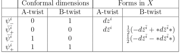
Now we will consider a Calabi-Yau 3-fold X as the target space. For the A-twist, the scalar fermionic fields have the structure of de Rham cohomology; and for the B-twist, Dolbeault cohomology, wherezi _{and ¯z}¯i _{are the coordinates of the Calabi-Yau}

Conformal dimensions Forms inX A-twist B-twist A-twist B-twist ψi

− 0 1 dzi

¯ ψ¯i

+ 0 0 dz¯i 12(−d¯z

¯_i

+∗dz¯¯i_∗)

¯ ψ¯i

− 1 0 12(−dz¯

¯_i

− ∗d¯z¯i_∗)

ψi

+ 1 1

Table 2.2: Cohomological structures under A- and B-twist

3-fold and∗ is the Hodge star with respect to the metric gi¯j.

For each twist, we can define a chiral ring of Q-closed operators. By convention, we say that an operatorO belongs to the (c, c) ring if

and the (a, c) ring if

[Q₋,O] = 0 [Q+,O] = 0. (2.16)

Operators in the (c, c) and (c, a) chiral rings can then be built up as

φ=ki1···ip¯j1···¯jqψ

i1

−· · ·ψ

ip −ψ

¯

j1 + · · ·ψ

¯

jq

+, (2.17)

ϕ=V j1···jq

¯_i1···¯_ip η

¯i1_{· · ·η}¯ip_θ

j1· · ·θjq, (2.18)

where η¯i _{= ¯ψ}¯i

++ ¯ψ ¯_i

− and θi =gi¯j( ¯ψ

¯_i +−ψ¯

¯

j

−). Define the tangent vector as ∂

∂zi∧=gi¯j ∗d¯z

¯_j

∗. (2.19)

The chiral ring then corresponds to cohomology Hp,q_{(X) and H}p

¯

∂(X,∧

q_T(1,0)_X),

re-spectively. According to the operator-state correspondence, the fields in the chiral rings also correspond to the supersymmetric ground states.

The twisted (2,2) sigma model is topological, because the variation of the action with respect to the worldsheet metric isQ-exact,

δ δgµν

S =Tµν = [Q,Λµν], (2.20)

and so it should not change the correlation functions. Unfortunately, the non-trivial correlation functions are limited to be the 3-point functions on a sphere and the partition function on a torus. If we want to obtain information for higher genus, we must couple the sigma model to gravity on the worldsheet, that is, we must allow for variation of the worldsheet metric. After doing that, the theory extends to a topological string theory.

2.3.1

U

(1)

anomaly

The reason that almost all correlation functions vanish in the topological sigma model is because of a U(1)R anomaly. As we know, a physical theory should not be

calculate the generating function, the measure of the fermionic fields is not invariant under chiral transformations. Therefore, theU(1) current associated to chiral symme-try is not a conserved current anymore. The divergence of the current is proportional to the difference between numbers of zero modes of chiral fermions. In mathematics, this difference is calculated by an index of the Dirac operator.

Since the correlation functions in the topological sigma model are independent of the metric of the Riemann surfaces, we can deform the metric by a scaling factor. When this factor goes to infinity, the action should be a minimum. This process is called localization. The path integral then picks up contributions only from the loci where the Q-variation of fermions vanishes [11]. In A-twisted sigma models, the Q-fixed point restricts the map from a worldsheet to target spaceX to be a holomorphic map; ¯∂¯zφ = 0. The anomaly is related to the index of the Dirac operator on the

worldsheet,

k= (2−2g) dimCX+c₁(X)·β, (2.21)

where β is the homology class of the map, β =φ_∗[Σ] ∈ H2(X,Z), c1(X) is the first

Chern class of X, and g is the genus of the worldsheet. When X is a Calabi-Yau manifold, c1(X) = 0, k is simplified to be (2−2g) dimCX.

In B-twisted sigma models, the Q-fixed point restricts the map to be a constant map, ∂µφ= 0, where ∂µ is a worldsheet derivative. The index is

k = (2−2g) dimCX. (2.22)

2.4

Closed topological string theory

Actually it was shown that a topological string on Calabi-Yau 3-fold has the same structure as a bosonic string theory in 26-dim. For example, for the correspondence of A-model topological string, see Table 2.3.

Bosonic string A-model topological string

QBRST QA

b ghost G+

energy-stress tensor T ={QBRST, b}, T ={QA, G+}

ghost number anomaly U(1)R anomaly

Table 2.3: Bosonic string vs A-model topological string

2.4.1

Bosonic string theory

The path integral for the bosonic string is over worldsheet inequivalent metrics of the gauge group,

diff×Weyl/CKG, (2.23)

where “diff” is the diffeomorphism group, “Weyl” is the Weyl group (scaling trans-formation of metric), and “CKG” is the conformal Killing group. We can use the Faddeev-Popov method to fix the gauge, which gives rise to an action for the b, c ghosts [12],

Sgh=

Z

d2_{zb∂c¯ +c.c. . (2.24)}

Similar to the chiral anomaly in a gauge theory, there is a ghost number anomaly from the difference between numbers of zero modes ofb and cghost. This number is equal to the dimension of the conformal Killing group κ, minus the dimension of the modular group µof the worldsheet. Using the Grothendieck-Riemann-Roch formula,

κ−µ= 3χ, (2.25)

dimension 3g−3. For g = 1 it has dimension 1, and for g = 0 it has dimension 0. The conformal Killing group for g > 1 has dimension 0; for g = 1 it has dimension 1, and for g = 0 it has dimension 3. Therefore, for g > 1, the path integral is just over the moduli space of the worldsheet. For g = 1 and 0, the topological string is the same as the topological sigma model. For g = 1, there is one modulus and one conformal Killing vector, so one operator insertion is needed in the path integral to fix this isometry. For g = 0, the non-zero physical quantities are the 3-point functions, with no moduli space left to integrate over. Forg >1 (g = 1), gauge fixing not only adds a ghost action to the original one, but also inserts µ (1) operators which are Beltrami differentials folded with 2-form supercurrents in the integrand. A Beltrami differential parametrizes a deformation of complex structure on the worldsheet. It is defined as

(µa)νµ =

1 2g

µρ_∂

agνρ, (2.26)

where a = 1,· · ·,3g −3 labels the deformations on the worldsheet and gµν is the

metric. In a complex coordinate system, it can be written as µ z

a¯z d¯z∂z, with µa ∈

H1 ¯

∂(Σ, T

(1,0)_Σ).

2.4.2

Closed topological string amplitudes

The correspondence between bosonic string theory and topological string theory al-lows us to write down the topological string amplitudes. Now the U(1)R anomaly

integrand; therefore, we are able to define topological string amplitudes [1] as

Fg =

Z Mg,h

[dm] *_3g−3

Y

a=1

Z

µaG−

Z ¯ µaG−

+

Σg,h

, (g >1) (2.27)

∂iF1 =

Z

F

dτ d¯τ Imτ

Z µG−

Z ¯

µG−O_i(1,1)

T2

, (2.28)

F1 =

Z

F

dτ d¯τ

Imτ T r(−1)

F_F

LFRqHLq¯HR, (2.29)

∂i∂j∂kF0 =

D

O(1_i ,1)O(1_j ,1)O_k(1,1)E

S2, (2.30)

where O_i(1,1) have U(1)R charge (1,1) ((left,right)).

2.4.3

Relation between closed topological strings and

physi-cal strings

Type II superstring theories have N = 2 supersymmetry in 10 dimensions. After compactification on a Calabi-Yau 3-fold only a quarter of the supersymmetry is pre-served, corresponding to N = 2 supersymmetry in 4 dimensions. The 4-dimensional theory contains one N = 2 supergravity multiplet, h1,1 _{+ 1 (h}2,1 _{+ 1) N = 2 vector}

multiplets, andh2,1_{+ 1 (h}1,1_{+ 1) hypermultiplets for A- (B-) type superstring theory,}

whereh1,1 _andh2,1 _{are the Hodge numbers of the Calabi-Yau 3-fold. The lowest}

com-ponents of the vector multiplets correspond to K¨ahler (complex structure) moduli of the Calabi-Yau 3-fold. Remarkably, the F-term of the low-energy effective theory is calculated by the closed topological string theory. This term is

X

g

Z d4x

Z

d4θFg(ti)W2g =

Z

d4xFg(ti)R+2F+2g−2, (2.31)

where W is the N = 2 supergravity multiplet, R+ is the curvature, F+ is the field

strength of the U(1) vector field component of W, ti _{are K¨ahler (complex}

struc-ture) moduli of the Calabi-Yau 3-fold, and Fg is exactly the closed topological string

Chapter 3

The Open Holomorphic Anomaly

Equation

3.1

Introduction

The closed holomorphic anomaly equation gives a recursion relation for the partition functionFg with respect to the genusg of the string worldsheet [1]. The equation has

proven to be useful in evaluating topological string amplitudes. In fact, for compact

Calabi-Yau manifolds, it is the only known method for computing these amplitudes systematically for higherg. This method has seen remarkable progress in recent years. The Feynman diagram method developed in [1] has been made more efficient by [13]. This, combined with the knowledge on the behavior of Fg at the boundaries of the

Calabi-Yau moduli space, has made it possible to integrate the holomorphic anomaly equation to very high values of g [14].

Recently, Walcher generalized the holomorphic anomaly equation to the case of topological string theory in the presence of D-branes [7]. Attempts to derive such an equation had been made before, for example in [1]. The new ingredients in [7] are two assumptions: that open string moduli do not contribute to factorizations in open string channels and that disk one-point functions vanish. A Feynman diagram method for integrating the holomorphic anomaly equation in the presence of D-branes has subsequently been proven [9] and enhanced [15, 16], as well as considered in the context of background independence [17]. Furthermore, initial attempts have been made to understand the situation where open string moduli may contribute [18].

on “wrong” moduli, that is complex structure moduli in the A-model and K¨ahler moduli in the B-model.

That disk one-point functions themselves depend on wrong moduli has been known for a long time. In [19], it was shown that D-branes in the A-model are associated to Lagrangian 3-cycles and that their disk one-point functions depend on B-model moduli. Conversely, D-branes in the B-model are associated to holomorphic even-cycles and their disk one-points functions depend on A-model moduli. One might then imagine that the disk one-point functions could introduce wrong moduli dependence into higher genus partition functions, and indeed we will find this effect explicitly, as a new type of anomalies in compact Calabi-Yau manifolds.

The cancellation of overall D-brane charge provides a means to remove the contri-bution of the new anomalies. Indeed, such a cancellation appears to be required for the successful counting of the number of BPS-states in M-theory using the topologi-cal string partition function. In [4], it was conjectured that the partition function of the closed topological string can be interpreted as counting BPS states in M-theory compactified to five dimensions on a Calabi-Yau 3-fold. This conjecture was extended to cases with D-branes in [5, 6]. Recently, Walcher [20] applied the formulae of [5] to examples of compactCalabi-Yau manifolds and found that the integrality of BPS state counting can be assured only when the topological charges of the D-branes were cancelled by introducing orientifold planes [20], such that the disk one-point functions vanish. Our result gives a microscopic explanation of this observation.

the presence of the new anomalies is correlated with the breakdown of large N du-ality. For compact Calabi-Yau manifolds, the conifold transition requires homology relations among vanishing cycles [22, 23]. For example, if a single 3-cycle of non-trivial homology shrinks and the singularity is blown up, the resulting manifold cannot be K¨ahler. Thus, the presence of D-branes with nontrivial topological charge implies a topological string theory without closed string dual; simultaneously the disk one-point functions do not vanish, so the new anomalies are present.

3.2

The open topological string theory

In this section, we will discuss some properties of the open topological string. We will write down the holomorphic anomaly equation and then prove it in Section 3.3.

3.2.1

Boundary condition

In order to preserve the scalar supercharge, there must be some boundary conditions for the supercurrents. We denote the supercurrentsG±_andG±_{, where barred} quanti-ties are right-moving, with conventions such that for both models the BRST operator is written as

QBRST =

I

G+_zdz + I

G+_z¯d¯z. (3.1) The appropriate worldsheet boundary conditions for the supercurrents are then

(G+_zdz+G+_z¯d¯z)|∂Σ = 0, and (G−zzχzdz+G

−

¯

zz¯χ¯z¯d¯z)|∂Σ = 0, (3.2)

where χ is a holomorphic vector along the boundary direction.

3.2.2

Some aspects of the moduli spaces of Riemann surfaces

• The Euler number for this manifold isχ=−(2g−2 +h+n+m/2).

• Since every handle is associated with 3 complex moduli, every boundary is associated with 3 real moduli, every marked point in the interior is associated with 2 real moduli, and every marked point on the boundary is associated with 1 real modulus. The dimension of the moduli space, is thus,

dimMg,h,n,m = 6g−6 + 3h+ 2n+m . (3.3)

• The boundary of the moduli space of Riemann surfaces corresponds to various degenerations of the surface (marked points are ignored). We use a set of cartoons in Figures 3.1–3.6.

• In the closed topological string theory, we need to insert a certain number of supercurrents folded with Beltrami differentials into the path integral on a worldsheet. These Beltrami differentials describe the complex deformations of the worldsheet. For a worldsheet with genusg and hboundaries, the dimension of the moduli space is 6g−6+3h, and this is the number of possible independent Beltrami differentials. To study the Beltrami differentials, we will double the Riemann surface Σg,h to be ˆΣ2g+h−1,0, such that boundaries of Σg,h are fixed

points of a_Z2 involution of ˆΣ2g+h−1,0; in other words,

Σg,h = ˆΣ2g+h−1/Z2. (3.4)

Mg−1,h

Figure 3.1: A handle pinches off, leaving Σg−1,h plus a degenerating

thin tube.

Mg1,h1 × Mg−g1,h−h1

Figure 3.2: An equator pinches off, splitting the Riemann surface into two non-trivial daughter surfaces Σg1,h2 and

Σg−g1,h−h1, joined by a degenerating thin

tube.

Mg1,h1 × Mg−g1,h+1−h1

Figure 3.3: A path from a boundary to the same boundary, around an equator, degenerates to leave two surfaces Σg1,h1 and

Σg−g1,h+1−h1, with the two

daugh-ter surfaces joined by a degenerat-ing thin strip.

Mg₋1,h+1

Figure 3.4: A path from a boundary to the same boundary, around a handle, degener-ates to leave Σg−1,h+1, with the two child

boundaries joined by a degenerating thin strip.

Mg,h−1

Figure 3.5: A path between two different boundaries degenerates, leaving Σg,h−1, with a

degenerat-ing thin strip across the newly-joined boundary.

Mg,h−1

3.2.3

Open holomorphic anomaly equation

Based on the previous discussion, the topological string partition function at a given genusg and boundary number h is written as

F(g,h) = Z

Mg,h

*_3g−3+h Y

a=1

Z

µaG−

Z ¯ µaG−

h

Y

b=1

Z

λb(G−+G−)

+

, (3.5)

whereµa (a= 1,· · · ,3g−3) are the Beltrami differentials associated with the moduli

of the bulk, µa (a = 3g −3 + 1,· · · ,3g −3 +h) are those associated with moduli

of the positions of the boundaries, and λb (b = 1,· · · , h) are those associated with

moduli of the length of the boundaries.

Our analysis below completes the derivation of [7], namely that under the as-sumption that open string moduli do not contribute to open string factorizations, for 2g−2 +h >0, we have a set of open holomorphic anomaly equations,

∂ ∂¯t¯iF

(g,h) ₌ 1

2C¯i¯j¯ke

2K_Gj¯j_Gkk¯ g

X

g1=0

h

X

h1=0

DjF(g1,h1)DkF(g−g1,h−h1)+DjDkF(g−1,h)

!

−eKGj¯j∆¯_i¯_jDjF(g,h−1), (3.6)

∂ ∂ypF

(g,h) ₌ ∂

∂y¯p¯F

(g,h)_{= 0, (3.7)}

if and only if

Cp¯=hω¯p¯|Bi= 0. (3.8)

HereB is the boundary and Cp¯ is a disk one-point function, with ¯ωp¯ an (a, a) chiral

primary state with chargesq¯a+ ¯q¯a=−3. If the disk one-point functions do not vanish,

3.3

New anomalies in topological string theory

In this section we will show how the new anomalies can enter (3.6) and (3.7) when the disk one-point functions do not vanish.

3.3.1

Physical meaning of the new anomalies

In quantum field theory, the vacuum expectation value of a field φat tree level is φcl.

The field is then expanded as,

φ=φcl+η, (3.9)

Figure 3.7: Tadpole

however the expectation value of φ may get quantum corrections through higher loops, i.e., hηi 6= 0. This is called a tadpole contribution. In order for the effective action method to work, the effective action Γ[φcl] should

not depend on the external current J. The effective action is defined as,

Γ[φcl] =

Z

d4xLren[φcl] +

i

2log det

−δ

2_Lren

δφδφ

−i(connect diagrams) + Z

d4xδL[φcl],

(3.10) whereLren is the renormalized Lagrangian. It was shown that a counterterm coming

from the currentδJ will cancel the tadpole contribution. δJ is the difference between J, the one which satisfies the equation of motion, andJren, the one which satisfies the

tree level equation of motion. Therefore we obtain a tadpole cancellation condition.

x

Figure 3.8: Disk one-point function

3.3.2

Anomalous worldsheet degenerations

In this section we consider the dependence of the genus g and boundary number h amplitude F(g,h) _{on both the anti-holomorphic moduli ¯t}¯i _{and the “wrong” moduli,}

labelledyp _{and ¯y}p¯_{. Our results are independent of choosing the A- or B-model; wrong}

moduli are complex structure moduli for the A-model and K¨ahler structure moduli for the B-model. To derive the extended holomorphic anomaly equation we follow the approach of [1], with the addition of some important details. Taking the ¯t¯i _derivative

of F(g,h) _{is equivalent to inserting the operator}

Z

Σ

{G+,[G+,φ¯¯_i]} (3.11)

into the amplitudes with the integral going over the worldsheet Σ. ¯φ¯_i is a state in the

(a, a) chiral ring with left- and right-moving U(1)R charge (−1,−1), which satisfies

[G−_,φ¯_¯

i] = 0 and [G

−

,φ¯¯_i] = 0. Here [G+,φ¯¯_i] means H_C

zdw G

+

(w) ¯φ¯_i(z), with Cz a

small contour surrounding z. In general the integrals of G+ _{and G}+ _{independently}

do not annihilate the boundary, so to derive the holomorphic anomaly we rewrite the insertion as

− 1

2 Z

Σ

{G++G+,[G+−G+,φ¯¯_i]}, (3.12)

allowing at least one contour to be deformed freely around the worldsheet.

For the other case, namely a dependence on wrong moduli, taking theyp_derivative

of F(g,h) _{is equivalent to inserting}

Z

Σ

{G+,[G−, ϕp]}+ 2

Z

∂Σ

ϕp, (3.13)

where ϕp is a charge (1,−1) marginal operator from the (c, a) ring, which satisfies

[G+, ϕp] = 0 and [G−, ϕp] = 0. The second term is a boundary term required to

resolve the so-called Warner problem [24]: we require the deformation to be Q-exact, but the Q variation of the first term alone is a boundary term, as can be seen using

{G+_{, G}−_{} = 2T and converting T to a total derivative. Since} R

Σ{G

+_,[G−_{, ϕ}

2R_∂Σϕp, we can rewrite (3.13) as

Z

Σ

{G++G+,[G−, ϕp]}, (3.14)

where again the first contour can be deformed past the boundaries on the worldsheet. Thus, for both the ¯t¯i andyp derivatives, the combination (G++G+) can be moved around the Riemann surface, and will produce terms corresponding to all possible degenerations of the Riemann surface, as listed below. For each degeneration, there also remain the insertions

¯

φ_¯(1)_i ≡ −1

2 Z

Σ

[G+_−G+_,φ¯

¯i], (3.15)

ϕ(1)_p ≡

Z

Σ

[G−, ϕp], (3.16)

for ¯t¯i _{and y}p _{dependence, respectively.}

Moving the contour of the supercurrent G+_+G+ _{around the Riemann surface,}

we pick up contributions from the commutation relations,

[G+, G−] = 2T, [G+, G−] = 2T . (3.17)

For the ¯t¯i _{derivative we then get}

¯

∂¯t¯iF(g,h)=− Z

Mg,h

[dm][dl]

"_3g−3+h X

c=1

¯ φ¯(1)_i

2

Z µcT

Z ¯

µcG−−2

Z

µcG−

Z ¯ µcT

×Y

a6=c

Z

µaG−

Z ¯ µaG−

h

Y

b=1

Z

(λbG−+ ¯λbG−)

+ + h X c=1 ¯ φ¯(1)_i

Z

2 λcT −λ¯cT

×

3g_Y−3+h a=1

Z

µaG−

Z ¯ µaG−

Y

b6=c

Z

(λbG−+ ¯λbG−)

+# .

For the yp _{derivative we just replace ¯φ}(1)

¯_i with ϕ(1)p . The insertions of the R µaT and

R ¯

µaT can be converted into derivatives with respect to the moduli ma and ma. By

Cauchy’s theorem, this reduces the integral over moduli space to contributions coming from the boundary of the moduli space, where we need to consider boundaries corre-sponding to degenerations of both the complex and real moduli, that is, both closed and open string degenerations. Equation (3.18) will then just sum the contributions from all the boundary components of moduli space.

To classify all boundary components of the moduli space of a Riemann surface with boundaries, a useful technique is to consider the degeneration, in turn, of all closed 1-cycles and open 1-paths with endpoints on (possibly distinct) boundaries. The various cases resulting from degenerations of closed 1-cycles were shown in Figures 3.1, 3.2, and 3.6, and of open 1-cycles in Figures 3.3, 3.4, and 3.5.

The first class of degenerations areclosed string factorizations, corresponding to a closed 1-cycle degenerating, and either removing a handle (Figure 3.1), or splitting the Riemann surface in two (Figure 3.2). The remaining modulus of the long, thin tube created is represented by an integrated (G−_−G−_{) insertion, folded with Beltrami} differential. This insertion annihilates the ground states propagating on the long tube, so for a non-zero result the remaining insertion (3.15) or (3.16) must also be on the tube. Now the absence of boundaries on the tube makes the results of BCOV [1] directly applicable. The long tubes project to two sets of ground states associated to two end points P_j¯_j|jigj¯jh¯j| and P_kk¯|kigkk¯hk¯|, where |ji is the topological twist

state, |¯ji is the anti-topological twist state, and gj¯j = hj|¯ji is the tt∗ metric. By

R-charge argument, the non-trivial contribution is from states in the (c, c) chiral ring with U(1)R charge (1,1). The yp derivative contributions vanish, and for the ¯t¯i

derivative we get two terms. The first term corresponding to Figure 3.1 is

1 2C¯i¯j¯ke

2K_Gj¯j_Gk¯k

Z Mg−1,h

[dm′] *Z

Σg−1,h

{G−,[G−, φj]}

Z

Σg−1,h

{G−,[G−, φk]}

×

3g_Y−6+h a=1

Z

µaG−

Z ¯ µaG−

h

Y

b=1

Z

(λbG−+ ¯λbG−)

+

where the set of moduli m′ _{correspond to the remaining Riemann surfaces Σ}

g−1,h.

The overall factor 1/2 results from the Z2 symmetry j ↔ k, Cijk is a three-point

function, namely the Yukawa coupling, and Gi¯i is the Zamolodchikov metric. This

expression can be further simplified. If we define

φ(2)_j = Z

Σg−1,h

{G−,[G−, φj]}, (3.20)

then the insertions φ(2)_j and φ(2)_k can be replaced by covariant derivativesDj and Dk

of the amplitude without insertions, namely of Fg−1,h. Therefore we get

1 2C¯i¯jk¯e

2K_G¯jj_G¯kk_D

jDkF(g−1,h). (3.21)

The second term corresponding to Figure 3.2 is

1 2C¯i¯jk¯e

2K_Gj¯j_Gk¯k g X r=0 h X s=0 Z Mr,s

[dm′] *

φ(2)_j

3r_Y−3+s a=1 Z

µaG−

2 _Ys b=1

Z

(λbG−+ ¯λbG−)

+

×

Z

Mg−r,h−s [dm′′]

* φ(2)_k

3(g−r_Y)−3+h−s a=1 Z

µaG−

2 h_Y−s b=1

Z

(λbG−+ ¯λbG−)

+

= 1 2C¯i¯j¯ke

2K_Gj¯j_Gk¯k g X r=0 h X s=0

DjF(r,s)DkF(g−r,h−s), (3.22)

where the sets of moduli m′ _{and m}′′ _{correspond to the remaining moduli on each of} the daughter surfaces. The overall factor 1/2 results from the Z2 symmetry of the

sum generated by simultaneously taking r → (g −r), s → (h−s), and j ↔ k. It is worth recalling that DjF(g,h) = 0 for 3g +h < 2, so there is no contribution for

sufficiently trivial daughter surfaces.

states. However, our assumption that open string moduli do not contribute removes all but charge 0 and 3 states, and these are annihilated by the G− _{or G}− _integrated around the attachment point, regardless of the location of the insertion (3.15) and (3.16). Thus the open string factorizations give gives no contribution.

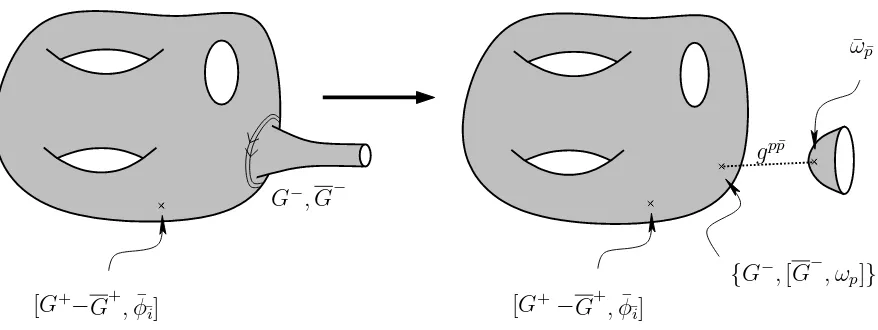
The last interesting case is that of a boundary shrinking, or equivalently moving far from the rest of the Riemann surface (Figure 3.6). That such a degeneration is part of the boundary of moduli space can be seen by doubling the Riemann surface Σg,h to form the closed surface Σ′2g+h−1,0, as described in Section 3.2.2. The pinching

off of a Σ′

2g+h−1,0 handle which crosses the Z2 fixed plane is equivalent to a shrinking

boundary in Σg,h.

This boundary is associated with three real moduli insertions, specifying the loca-tion of the boundary and its lengthτ. The boundary degeneration is thus equivalent to a boundary at the end of a long tube, with the Beltrami differentials associated with the two remaining moduli localized to the attachment point of the tube to the rest of the Riemann surface. The absence of additional moduli on the tube distin-guishes this class from the closed string factorization class above, and furthermore allows the remaining insertion (3.15) and (3.16) to be anywhere on the worldsheet.

Firstly, insertions (3.15) and (3.16) may be on the tube. The degenerationτ → ∞

projects the intermediate states on both sides of the insertion to ground states, since excited states decay as e−hτ _{where h >0 is the total (left+right) conformal weight.}

Now, however, G± _{and G}± _{annihilate the ground states, so this case is zero.}

Secondly, the insertions may be near the shrinking boundary. The tube pinching off in the middle gives rise to a disk Σ0,1 and the remaining Riemann surface Σg,h−1.

This will project to one set of ground states P_j¯_j|jigj¯jh¯j| on the pinching off point.

For the ¯t¯i _{derivative, the disk part gives us}

− 1

2e

K_Gj¯j_h¯j|

Z

Σ0,1

Define the anti-topological disk two-point function as

∆¯_i¯_j = 1

2h¯j| Z

Σ0,1

[G+−G+,φ¯¯_i]|Bi. (3.24)

The remaining Riemann surface Σg,h−1 then has a φ(2)j insertion, which produces

DjF(g,h−1). Multiplying the two contributions, we obtain

−eKGj¯j∆¯_i¯_jDjF(g,h−1). (3.25)

For the yp _{derivative, the near-boundary region is shown in Figure 3.9. We can}

replace the tube with a complete set of closed-string ground states, P_I,J¯|IigIJ¯hJ¯|,

wheregIJ¯_{is thett}∗ _{metric, andI, ¯J run over all (c, c) and (a, a) chiral primary states,} respectively. Standard considerations of global consistency on the Riemann surface force |Ii = |ii to be a charge (1,1) ( i.e., marginal) state, and hJ¯| = h¯j| to be a charge (−1,−1) state from the (a, a) chiral ring. Near the boundary the theory is anti-topologically twisted, making G− _{and G}− _{of dimension 1 as supercurrents, and} so allowing contour deformation. Using the properties of the chiral rings, (3.16) can be written as R_Σ[G−_+G−_{, ϕ}

p]. The contour of (G− +G−) can be deformed off the

disk, annihilating both h¯j| and the boundary, so this case is zero.

Lastly, (3.15) and (3.16) may be inserted somewhere else on the Riemann surface, as shown in Figures 3.10 and 3.11 for the yp _{and ¯t}¯i _{derivatives, respectively. The}

tube is again replaced with a complete set of ground states P_I,J¯|IigIJ¯hJ¯|. To avoid

annihilation byG−_andG− _{localized to the tube attachment point,|Iimust be in the} (c, c) chiral ring and haveqI,q¯I 6= 0. Furthermore, both of the insertions (3.15) and

(3.16) are (linear combinations of) states with (0,−1) or (−1,0) left- and right-moving U(1)R charge, and the tube end-point moduli contribute charge (−1,−1), so |Ii is

required to be a (linear combination of) charge (1,2) or (2,1) states. We denote these states ωp, with index p running over charge (1,2) and (2,1) chiral primaries. Note

that the ωp are not associated with marginal deformations of the topological string

[G−_{, ϕ}

p] h¯i|= ¯φ¯_i

Figure 3.9: The near-boundary re-gion of the shrinking boundary de-generation for yp _{derivative, with}

insertion (3.16) near the bound-ary. This amplitude vanishes, as described in the text.

{G−,[G−, ωq]}

[G−, ϕp]

¯ ωq¯

gqq¯

Figure 3.10: Amplitude for the shrinking boundary degeneration for yp _derivative,

with insertion (3.16) elsewhere on the Rie-mann surface. This is non-zero unless the disk one-point function vanishes.

¯ ωp¯

[G+₋

G+,φ¯¯_i]

[G+₋

G+,φ¯¯_i]

G−_{, G}−

{G−,[G−, ωp]}

gpp¯

Figure 3.11: Amplitude for the shrinking boundary degenerating for ¯t¯i _derivative,

with the insertion (3.15) located away from the shrinking boundary. On the right we have replaced the tube with a sum over statesωa of charge (1,2) and (2,1), rendering

target space 3-forms, and hence to complex structure variation, and in the B-model they are (1,1) forms, and so correspond to K¨ahler deformations. Near the shrinking boundary the resulting amplitude is the disk one-point function,

Cp¯=hω¯p¯|Bi. (3.26)

This amplitude is in general not zero, and indeed our boundary conditions are such that the disk one-point function is only non-zero when the closed string state is from the wrong model [19]. This case thus contributes the following new terms to (3.6) and (3.7): for the derivative with respect to ¯t¯i_,

gpq¯ Cp¯

Z Mg,h−1

[dm′] *Z

Σg,h−1

{G−,[G−, ωq]}

Z

Σg,h−1

[G+−G+,φ¯¯_i]

+

Σg,h−1

, (3.27)

and for the derivative with respect to yp_,

gpq¯ Cp¯

Z Mg,h−1

[dm′] *Z

Σg,h−1

{G−,[G−, ωq]}

Z

Σg,h−1

[G−, ϕp]

+

Σg,h−1

, (3.28)

where the m′_{s are the moduli of the Riemann surface Σ}

g,h−1—the corresponding

insertions of G− _{and G}− _{folded with Beltrami differentials have been suppressed.} Note that theG− _andG− _{contours aroundω}

q and ϕp cannot be deformed as they are

dimension 2 as supercurrents and that the (G+_−G+_{) contour around ¯φ}

¯_i cannot be

deformed as it does not annihilate any additional boundaries that may be present.

3.4

Small number of moduli

We have so far discussed the holomorphic anomaly equation for 2g−2 +h >0. For low-genus and low-boundary cases, that is 2g−2 +h ≤0, F(1,0) _{does not have new}

anomalies [1], while F(0,2) _{has new anomalies similar to those discussed above.}

F(0,0) _{and F}(0,1) _{are sphere and disk amplitudes, but since neither the sphere nor}

3.4.1

Cylinder

Σ

L

Figure 3.12: Cylinder

The open string 1-loop partition function is denoted as F(0,2)_{. Quantum mechanically, if an open string state}

|αi evolves to a state |βi = e−iHt_{|αi, the amplitude}

from|αito|βiishβ|αi. After applying a wick rotation along the time direction, we obtain a partition function T re−HL_{|αihα|. In terms of a sigma-model on a}

Calabi-Yau 3-fold, we can compute this partition function. Since there is only one real modulus and one isometry associated to the circular direction, we can write down the amplitude

F(0,2) = Z

dL

L T r[(−1)

F_{F e}−LH_{], (3.29)}

where F is the U(1)R current, L is the modulus of the cylinder and H is the

Hamil-tonian for the string. The derivative with respect to a modulus of the Calabi-Yau is

∂ ∂tjF

(0,2) ₌

Z _dL L

*Z

Σ0,2

{G−_,[G−_{, φ}

j]}F

+

. (3.30)

The holomorphic anomaly equation is

∂ ∂t¯¯i

∂ ∂tjF

(0,2) ₌

Z 1 0

dL L

*Z

Σ0,2

{G+,[G+,φ¯¯_i]}

Z

Σ0,2

n

(G−+G−), φ(1)_j oF +

, (3.31)

where φ(1)_j is a 1-form and ¯φ¯i is a (1,1) form on the cylinder. We will then use

commutation relations,

[F, G−_{] = G}−_{, [F, G}−_{] =G}−_{, [F, φ}

j] = 0, (3.32)

to get that the relevant insertions on the degenerate Riemann surfaces are ¯φ¯[1]_i and

φ(1)_j , where ¯φ¯[1]_i is a U(1)R charge −1 operator and φ(1)j is a charge 1 operator. Let’s

consider three types of degenerations.

X X

i

j

Figure 3.13: Blow up of the colliding of two operators

ii) Since a cylinder is conformally equivalent to an annulus, there is another kind of degeneration corresponding to two boundaries of the annulus colliding (Figure 3.14) and producing a long and narrow strip. The only non-trivial degeneration is when

¯

φ¯[1]i and φ

(1)

j are both away from the strip, and we project the strip to open string

ground states. By the charge argument and also the assumption of a non-trivial open string ground state, we can just insert open string ground states with charges 0 and 3. It was discovered [1] that

*

Oα

Z

C

φ(1)_j Z

Σ0,1

¯ φ¯[1]_i Oβ

+

=−Ri¯jαβ. (3.33)

where O denotes a U(1) charge 0 open string ground state, and D is the degeneracy of the states. Since φ(1)_j is a one-form on the disk, it must be integrated along a path C.

X

XX X X

X

¯

φ_¯[1]_i φ(1)_j

Oα

Oα

Oβ

Oβ

Figure 3.14: Boundary colliding

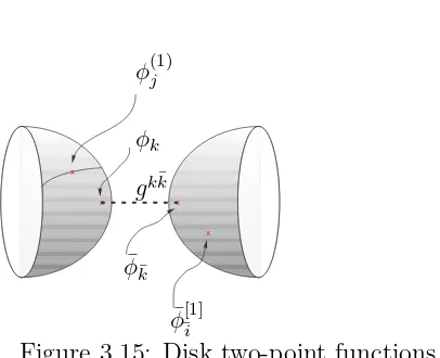
iii) Cylinder splitting. If ¯φ¯[1]i and φ

(1)

j are inserted at opposite ends of this

x x

x

x

¯

φ_¯[1]_i φ(1)_j

φk

¯

φ¯_k

gkk¯

Figure 3.15: Disk two-point functions

states which stay in the (c, c) or (a, a) rings with charge (1,1) or (−1,−1). Recall the definition of disk two-point function (3.24), we get

Z

C

φ(1)_j φk

gk¯k

*Z

Σ0,1

¯ φ_¯[1]_i φ¯¯_k

+

= ∆jk∆¯_i¯_keKGk¯k. (3.34)

If ¯φ¯[1]_i and φ(1)j are inserted on the same side (Figure 3.16), then by the charge

argu-ment, we have to project to ground states ωp which stay in the (c, c) ring of charge

(1,2) and (2,1). The three-point function on the disk is *Z

C

φ(1)_j Z

Σ0,1

¯ φ¯[1]_i ωp

+

. (3.35)

If the disk one-point function does not vanish, we obtain a wrong moduli dependent term

gpp¯ Cp¯

*Z

C

φ(1)_j Z

Σ0,1

¯ φ¯[1]_i ωp

+

, (3.36)

where Cp¯ is defined as (3.26). When the disk one-point functions vanish, we get the

holomorphic anomaly equation for a cylinder, ∂

∂¯t¯i

∂

∂tjF0,2 =e

K_Gi¯j_∆

¯_i¯_j∆ij +

D

2G¯ij. (3.37)

Since φ(1)_i , ϕ(1)p ; ¯φ¯(1)i , ¯ϕ

(1) ¯

p have charges 1 and −1, respectively, the requirement of

x x x

x

¯

φ_¯[1]_i φ(1)_j

ωp

¯

ωp¯

gpp¯

Figure 3.16: Disk one-point function

∂¯_i∂pF(0,2), ∂i∂p¯F(0,2), and ∂p¯∂qF(0,2). Correspondingly, the insertions are ¯φ¯[1]_i ϕ (1)

p ,

φ(1)_i ϕ¯[1]p¯ , and ¯ϕ [1] ¯

p ϕ

(1)

q . We can repeat the same discussion and find that the only

contribution comes from the disk one-point functions, and therefore the vanishing of the disk one-point function makes them all zero.

3.4.2

Some discussion

The derivation above may not seem to distinguish between compact and non-compact Calabi-Yau target spaces. In fact, the anomalies can only appear in the compact case. Beforehand, note that this agrees with our expectations: D-branes wrapped on cycles in compact Calabi-Yau manifolds and filling spacetime (or perhaps even two directions in spacetime [20]) give an inconsistent setup unless there are sinks for the topological D-brane charges. Simultaneously, these sinks cancel the disk one-point functions, and so the appearance of the new anomalies is correlated with an invalid spacetime construction.

Furthermore, the standard results of Chern-Simons gauge theory and matrix mod-els as open topological string theories are not affected by the new anomalies. For example, N D-branes wrapping the S3 _{of the space T}∗_S3_{, gives C}

¯

p 6= 0. The total

space of T∗_S3 _{is Calabi-Yau and non-compact, with the S}3 _{radius as the complex}

structure modulus. It is well-known that open topological string theory on this space is theU(N) Chern-Simons theory, which is topological and should be independent of the S3 _{radius. To resolve this apparent contradiction, consider embeddingT}∗_S3 _{in a}

wrapped byN anti-D-branes. The boundary states of the two stacks combine to give Cp¯= 0, and the new anomalies do not appear. Now take the limit where the second

3-cycle moves infinitely far away from the base S3 _{to recover an anomaly-free local}

Calabi-Yau construction. The point is that in non-compact Calabi-Yau manifolds, the new anomalies can be removed by an appropriate choice of boundary conditions at infinity.

3.5

Feynman rules to solve the holomorphic anomaly

equation

The series of open holomorphic anomaly equations without new anomalies are

∂ ∂¯t¯iF

(g,h) ₌ 1

2C¯i¯j¯ke

2K_Gj¯j_Gkk¯ g

X

r=0

h

X

s=0

DjF(r,s)DkF(g−r,h−s)+DjDkF(g−1,h)

!

−eKGj¯j∆¯_i¯_jDjF(g,h−1), (3.38)

∂ ∂ti

∂ ∂¯t¯jF

(1,0) ₌ 1

2CikℓC¯jk¯ℓ¯e

2K_Gk¯k_Gℓ¯ℓ₋₍χ

24−1)Gi¯j, (3.39) ∂

∂t¯¯i

∂ ∂tjF

(0,2) _=eK_Gi¯j_∆

¯_i¯_j∆ij +

N

2G¯ij. (3.40)

Now we discuss the solution to these holomorphic anomaly equations. The moduli space of a Calabi-Yau 3-fold enjoys K¨ahler geometry. There exists a line bundle L

over it corresponding to rescalings of the K¨ahler potentialK. TheF(g,h)_{’s are sections}

of this line bundleL2−2g−h_{, so the covariant derivatives on this line bundle are defined}

as

Di =∂i −(2−2g−h)∂iK. (3.41)

rules. Firstly, we define the propagators [1] −S, −Sj_{, and −S}jk_{, where}

S, such that C¯_i¯_j¯_k=e−2KD¯_iD¯_j∂¯¯_kS, (3.42)

Sj =Gj¯jS¯_j, where S¯_j = ¯∂¯_jS, (3.43)

Sjk =Gj¯jS¯_jk, where S¯_jk = ¯∂¯_jSk, (3.44)

and the terminators [7]

∆, such that ∆¯i¯j =e−KD¯i∂¯j∆, (3.45)

∆j =Gj¯j∂¯j∆. (3.46)

Feynman diagrams for those propagators and terminators are given in Figure 3.17.

X

X X X X X

X X

Sij _Si _S

∆i _∆

Figure 3.17: The propagators for Feynman diagrams of topological string amplitudes

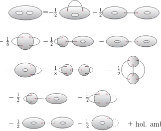
The low-genus and boundary cases,F(2,0)_,F(3,0)_,F(1,1)_{, andF}(0,3)_{, were studied in}

[1] and [7]. For example, for genus 2, the amplitudes is determined up to a holomorphic ambiguity,

F(2,0) = 1 2S

ij_C(1)

ij +

1 2C

(1)

i SijC

(1)

j −

1 8S

jk_Smn_C jkmn−

1 2S

ij_C

ijmSmnCn(1)

+ 1 8S

ij_C

ijpSpqCqmnSmn+

χ 24S

i_C(1)

i +

1 12S

ij_Spq_Smn_C

ipmCjqn−

χ 48S

i_C ijkSjk

+χ 24(

χ

24 −1)S+ hol. amb., (3.47)

where

C_i(₁g_···)_in ≡ Di1· · ·DinF

(g,0)_{, (3.48)}

C_ϕ(1) ≡ χ

and the Yukawa coupling Cijk can be interpreted as the building blocks of the

Feyn-man diagrams (Figure 3.18).

X X X X X X X X X X X X X X X X X X X X X X X X X X X X X X X X X X

=

−

2

−

−

−

−

−

−

8

−

−

−

−

−

2

+ hol. amb.

Figure 3.18: Feynman diagrams forF(2,0)

For genus 1 with 1 boundary, the amplitude is

F(1,1) = 1 2S

jk_∆jk−C(1)

j ∆j+

1 2CjklS

kl_∆j₋₍χ

24−1)∆ + hol. amb.. (3.50) We can draw Feynman diagrams as Figure 3.19.

x x x x x x x

=

−

2

−

−

1

2

−

+ hol. amb.

Chapter 4

The Relation between the Open and

Closed Topological String

In this chapter we show that a general solution to the extended holomorphic anomaly equations for the open topological string on D-branes in a Calabi-Yau manifold, re-cently written down by Walcher [7], is obtained from the BCOV solution to the holomorphic anomaly equations for the closed topological string on the same mani-fold [1], by shifting the closed string moduli by amounts proportional to the ’t Hooft coupling [9].

4.1

Generating function

In Chapter 3, we derived the open holomorphic anomaly equations. The extended equation for the string amplitudes with closed-string operator insertions [7] is

¯

∂¯_iF_i(₁g,h_,···)_,in = 1

2 X

g1+g2=g

h1+h2=h

C¯jk_i

X

s,σ

1 s!(n−s)!F

(g1,h1)

jiσ(1),···,iσ(s)F (g2,h2)

kiσ(s+1),···,iσ(n) +

1 2C

jk

¯_i F_jki(g−₁1_,···,h_,i)_n

−∆¯j_iFji(g,h1,···−,i1)n −(2g−2 +h+n−1)

n

X

s=1

Gis¯iF

(g,h)

i1,···,is−1,is+1,···,in. (4.1)

The last term comes from the collision of two closed-string marginal operators [1], since

Gi¯j =hφ

(2)

i φ¯

(2)

¯j iΣ0,0, (4.2)

where

φ(2)_j = Z

Σg,h

{G−,[G−, φj]}. (4.3)

The ingredients F_i(₁g,h_,...,i)_n are topological string amplitudes with worldsheet genusg, h boundaries, andninsertions of closed-string marginal operators indexed byi1,· · · , in;

also C¯jki =C¯i¯j¯ke2KGj

¯

j_Gkk¯_{, where C}

¯_i¯_j¯_k is the Yukawa coupling, indices are raised and

lowered using the Zamolodchikov metric Gi¯j = ∂i∂¯_jK, and ∆_¯ij = eKGj¯k∆¯_i¯_k, where

∆¯_i¯_k is the disk two-point function. Note that these are different from the ∆ (with or

without indices) that appear in BCOV, which we will denote as ˆ∆ below.

Following BCOV, we define the generating function for open topological string amplitudes,

W(x, ϕ;t,¯t) = X

g,h,n

1 n!g

2g−2

s λhF

(g,h)

i1,···,inx

i1_{· · ·x}in

1 1−ϕ

2g−2+h+n

+

χ

24−1− D

2g −2

s λ2

log

1 1−ϕ

, (4.4)

where the sum is over g, h, n≥0 such that (2g−2 +h+n)>0,gs is the topological

string coupling constant, andλis the ’t Hooft coupling constant, namelygs times the

topological string Chan-Paton factor. In the last term on the right, χ is the Euler characteristic of the Calabi-Yau manifold andDis the number of open-string ground states with zero charge. This term contributes to the holomorphic anomaly equations for F_i(1,0) and F_i(0,2), reproducing [2]

∂ ∂ti

∂ ∂¯t¯jF

(1,0) ₌ 1

2CiklC¯jk¯¯le

2K_Gkk¯_Gl¯l₋χ

24−1

Gi¯j (4.5)

and [7]

∂ ∂ti

∂ ∂¯t¯jF

(1,0) ₌ 1

2∆ik∆¯jk¯e

K_Gkk¯₋ D

2Gi¯j. (4.6) We will show this in the Appendix A.1. The generating function W satisfies an extension of Equation (6.11) in BCOV by a λ-dependent term, namely

∂ ∂¯t¯ie

W(x,ϕ;t,t¯) ₌

g2

s

2C

jk

¯_i ∂

2

∂xj_∂xk −G¯ijx j ∂

∂ϕ −λ∆

j

¯_i

∂ ∂xj

eW(x,ϕ;t,¯t), (4.7)

for each genus and boundary number.

Our key result is that Equation (4.7) can be rewritten in the same form as the closed topological string analogue by simply shifting

xi →xi+λ∆i, ϕ→ϕ+λ∆, (4.8)

where ∆i _{and ∆ are defined implicitly, modulo holomorphic ambiguities, by ∆}

¯

i¯j =

e−K_G

¯

jk∂¯i∆k=e−KD¯iD¯j∆. After this shift Equation (4.7) becomes,

∂ ∂¯t¯ie

W(x+λ∆,ϕ+λ∆;t,t¯) ₌

g2

s

2C

jk

¯_i ∂

2

∂xj_∂xk −G¯ijx j ∂

∂ϕ

eW(x+λ∆,ϕ+λ∆;t,¯t). (4.9)

This is exactly the same as the original BCOV equation for the closed topological string generating function, with theµ-dependent term absorbed by means of the shift (4.8).

Our result follows from a straightforward application of the chain rule: noting that ¯∂¯i∆j = ∆¯j_i, the variable shift produces two new terms on the left,

λ∆¯j_i

∂

∂xj +λ∆¯i

∂ ∂ϕ

eW. (4.10)

The first is the additional µ-dependent term on the right of (4.7). Using G¯_ij∆j =

∆¯_i, the second term combines with the second term on the right of (4.9) to give

−G¯_ij(xj +λ∆j)_∂ϕ∂ eW, which is required for matching powers of x+λ∆ in the

ex-pansion of the generating function. Thus we have reproduced the open topological string holomorphic anomaly equations from the closed topological string holomorphic anomaly equations, simply by a shift of variables.

rules. Equation (6.12) in BCOV defines the function

Y(x, ϕ;t,¯t) = − 1

2g2

s

( ˆ∆ijxixj+ 2 ˆ∆iϕxiϕ+ ˆ∆ϕϕϕ2) +

1 2log

det ˆ∆ g2

s

!

, (4.11)

where the ˆ∆ij are the inverses of the corresponding propagators Sij. Expanding

Z = R dxdϕexp(Y +W) in powers of gs then produces the full Feynman diagram

expansion of the closed topological string amplitudes. The shift (4.8) produces the additional terms appearing in the open string Feynman diagrams, shown in Section 2.10 of Walcher. Therefore the Feynman rules method in Section 3.5 is generalized to solve the open holomorphic anomaly equations. In field theory language, the shift effectively generates the vacuum expectation values hxi_{i = ∆}i _{and hϕi = ∆, and so}

terms containing ∆i _{and ∆ correspond to diagrams with tadpoles.}

4.2

The closed string moduli and coupling

The shift we use above is, strictly speaking, a shift of the variables x and ϕ, rather than the closed-string moduli t and gs. Howeve