Adaptive Radial Basis Function Detector for
Beamforming
Sheng Chen, Khaled Labib, Rong Kang and Lajos Hanzo
School of Electronics and Computer ScienceUniversity of Southampton, Southampton SO17 1BJ, UK E-mails:{sqc,koml105,rk405,lh}@ecs.soton.ac.uk
Abstract— We consider nonlinear detection in rank-deficient multiple-antenna assisted beamforming systems. By exploiting the inherent symmetry of the underlying optimal Bayesian detection solution, a symmetric radial basis function (RBF) detector is proposed and two adaptive algorithms are developed for training the proposed RBF detector. The first adaptive algorithm, referred to as the nonlinear least bit error, is a stochastic approximation to the Parzen window estimation of the detector output’s probability density function while the second algorithm is based on a cluster-ing. The proposed adaptive solutions are capable of providing a signal to noise ratio gain in excess of 8 dB against the theoretical linear minimum bit error rate benchmarker, when supporting four users with the aid of two receive antennas or five users employing three antenna elements.
I. INTRODUCTION
Adaptive beamforming is capable of separating user signals transmitted on the same carrier frequency, and thus provides a practical means of supporting multiusers in a space-division multiple-access scenario [1]–[10]. Classically, this is achieved by a linearbeamformer based on the minimum mean square error (L-MMSE) solution [1],[2],[7],[8],[11]. The L-MMSE beamforming requires that the number of users supported is no more than the number of receive antenna elements. If this condition is not met, the system is referred to as overloaded or rank-deficient. The optimal solution for the linear beamforming has been shown to be the minimum bit error rate (L-MBER) design [12],[13] which outperforms the L-MMSE one and is capable of operating in hostile rank-deficient scenarios. However, digital communication signal detection can be viewed as a classification problem [14]-[16], where the receiver detector simply classifies the received multidimensional channel-impaired signal into the most-likely transmitted symbol constellation point or class. Both the radial basis function (RBF) network [17]-[19] and other kernel models [20]-[25] have been applied to solve this nonlinear detection problem. All these nonlinear detectors attempt to approximate the underlying optimal Bayesian solution. The standard RBF or kernel modelling technique constitutes a black-box approach that seeks to extract a model representa-tion from the available training data. Adopting this black-box modelling approach is appropriate, if no a prioriinformation exists regarding the underlying data generating mechanism. If however there exists some a prioriinformation concerning the system to be modelled, this a priori information should be incorporated into the modelling process. Many real-life
phenomena exhibit inherent properties, such as symmetry, but these properties are often hard to infer from the data with the aid of black-box models. In regression modelling, the symmetric properties of the underlying system have been exploited by imposing symmetry in both RBF networks and least squares support vector machines [26],[27]. By imposing symmetry on the model’s structure, it is easier to extract the inherent symmetry properties of the underlying system from noisy training data and this leads to substantial improvements in the achievable regression modelling performance. In this paper, we propose a symmetric RBF detector for multiple-antenna aided beamforming systems.
The optimal Bayesian nonlinear detection solution has an inherent symmetry because the signal states corresponding to the different signal classes are distributed symmetrically. This symmetric property is difficult to infer from noisy training data using a standard RBF model. In fact, previous studies [16]-[25] have shown that a standard RBF detector typically requires significantly more RBF centres than the number of channel output states in order to approximate the Bayesian detector using noisy training data, and often there is a performance difference between such a RBF detector and the optimal Baysian solution. In contrast to the standard RBF model, the proposed symmetric RBF model is capable of approaching the optimal Bayesian performance accurately, despite using channel-impaired training data and despite using no more RBF centres than the number of channel output states. The advantage of the proposed symmetric RBF detector is demon-strated in challenging detection scenarios, where the number of users supported is almost twice the number of antenna array elements. Two adaptive algorithms are developed to update the symmetric RBF detector’s parameters on a sample-by-sample basis for the sake of maintaining a low real-time computational complexity. The first adaptive algorithm is a stochastic learning algorithm, referred to as the nonlinear least bit error rate (NLBER), which directly minimises an approximate detection error probability or bit error rate (BER). The second adaptive algorithm is based on the enhanced κ -means clustering algorithm [16].
II. MULTIPLEANTENNAASSISTEDBEAMFORMING
The system supports M users, where each user transmits on the same carrier frequency of ω = 2πf, and the receiver is equipped with a linear antenna array consisting of L
uniformly spaced elements. Further assume that the channel is non-dispersive. Then the symbol-rate complex-valued received signal samples can be expressed as
xl(k) = M
i=1
Aibi(k)ejωtl(θi)+nl(k) = ¯xl(k) +nl(k), (1)
for 1 ≤ l ≤ L, where tl(θi) is the relative time delay at array element l for source i, with θi being the direction of arrival for source i, nl(k) is the Gaussian white noise with E[|nl(k)|2] = 2σn2,Ai is the channel coefficient of useri, and bi(k)is thek-th symbol of useri, taking values from a binary phase shift keying (BPSK) symbol set, i.e. bi(k) ∈ {±1}. Source 1 is the desired user and the rest of the sources are the interfering users. The desired user’s signal-to-noise ratio is given by SNR=|A1|2σb2/2σ2n, whereσ2b = 1 is the BPSK symbol energy, and the desired signal-to-interferer i ratio is defined by SIRi=|A1|2/|Ai|2, for 2≤i≤M. The received signal vector x(k) = [x1(k)· · ·xL(k)]T can be expressed as
x(k) =Pb(k) +n(k) = ¯x(k) +n(k), (2) where n(k) = [n1(k)· · ·nL(k)]T and the system matrix P is given by P= [A1s1· · ·AMsM]with the steering vector of sourceigiven bysi=ejωt1(θi)· · ·ejωtL(θi)T, and the trans-mitted BPSK symbol vector byb(k) = [b1(k)· · ·bM(k)]T. Traditionally, a linear beamforming receiver, yLin(k) = θTx(k), is adopted to detect the desired user’s signal [1],[7]
with the associated decision given by
ˆ
b1(k) =sgn([yLin(k)]) =
+1, [yLin(k)]≥0, −1, [yLin(k)]<0, (3) where θ = [θ1· · ·θL]T denotes the complex-valued linear beamformer’s weight vector and[•]the real part. Classically, the L-MMSE solution for the weight vector of the linear beam-former is regarded as the optimal design [1],[2],[7],[8],[11]. The L-MMSE technique requires that the number of usersM is no higher than the number of antenna array elementsL. The optimal weight vector designed for the linear beamformer is known to be the L-MBER solution [12],[13] which directly minimises the BER of the linear beamformer and is capable of operating in rank-deficient scenarios.
However, the optimal multiple antenna aided beamforming detector is nonlinear [16],[25]. Let us denote the Nb = 2M combinations of b(k) as bq, 1 ≤ q ≤ Nb, and the first element ofbq, related to the desired user, asbq,1. The noiseless channel output x¯(k) takes values from the finite signal set ¯
x(k)∈ X ={x¯q =Pbq,1≤q≤Nb}, which can be divided into two subsets conditioned on the value of b1(k)as
X(±)={x¯
i∈ X,1≤i≤Nsb: b1(k) =±1}, (4)
where the size ofX(+)andX(−)isNsb=Nb/2 = 2M−1. Let the conditional probabilities of receivingx(k)givenb1(k) = ±1 bep±(x(k)) =p(x(k)|b1(k) =±1). According to Bayes decision theory [28], the optimal detection strategy is
ˆb1(k) = +1, if p+(x(k))≥p−(x(k)),
−1, if p+(x(k))< p−(x(k)). (5)
If we introduce the real-valued Bayesian decision variable
yBay(k) =fBay(x(k))= 1
2p+(x(k))− 1
2p−(x(k)), (6) the optimal detection rule (5) is equivalent to ˆb1(k) = sgn(yBay(k)). Decision variable (6) can be expressed as
yBay(k) =
Nb
q=1
sgn(bq,1)βqe−
x(k)−x¯q2
2σ2n (7)
where βq denotes the a priori probability of x¯q. Since all the x¯q are equiprobable, βq = β = N 1
b(2πσ2n)L. The two subsetsX(+)andX(−)are distributed symmetrically, namely, for any signal state ¯x(+)i ∈ X(+) there exists a signal state ¯
x(i−)∈ X(−) satisfyingx¯(−)
i =−¯x(+)i . Given this symmetry,
the optimal Bayesian detector (7) can be characterised as
yBay(k) =
Nsb
q=1
βq
e−
x(k)−¯x(+)q 2
2σ2n −e−
x(k)+¯x(+)q 2
2σ2n
, (8)
wherex¯(+)q ∈ X(+). The Bayesian detector hasoddsymmetry, as fBay(−x(k)) = −fBay(x(k)). This symmetry is hard to infer from the noisy data by a standard RBF detector.
III. SYMMETRICRADIALBASISFUNCTIONDETECTOR Consider the training of the RBF detector of the form
yRBF(k) =fRBF(x(k);w) =
nc
i=1
θiφi(x(k)), (9)
based on the training data setDK ={x(k), b1(k)}Kk=1, where f(•;•)is a real-valued nonlinear mapping realised by the RBF network,θi is theith real-valued RBF weight,φi(•)denotes the response of thei-th RBF node, nc is the number of RBF nodes used, and w denotes the vector of all the adjustable parameters of the RBF detector. We propose to adopt the following symmetric RBF node
φi(x)=ϕ(x;ci, σi2)−ϕ(x;−ci, σi2), (10) where ci is the ith complex-valued RBF centre, σ2i the ith real-valued RBF variance, andϕ(•)the classic RBF function. In this study we adopt the Gaussian RBF function
ϕ(x;ci, σ2) =e−
x−ci2
σ2 . (11)
The symmetric RBF network (9) with the node structure (10) has an inherently odd symmetry. A standard RBF model with the RBF node defined by φi(x)= ϕ(x;ci, σ2i), by contrast, cannot guarantee odd symmetry, particularly when the RBF centres are generated from noisy training data.
A. The nonlinear least bit error rate algorithm
Let us define the signed decision variable ys(k) = sgn(b1(k))yRBF(k) and denote the probability density func-tion (PDF) ofys(k) as py(ys). Then the error probability of the nonlinear detector (9) is given by
PE(w) =Prob{ys(k)<0}= 0
The MBER solution for the detector’s parameter vector w is defined as the one that minimises PE(w). The problem with this approach is that the PDF ofys(k)is unknown. However, it may be sufficiently accurately estimated using the Parzen window method [29]-[31]. Given a block of training dataDK, a Parzen window estimate of py(ys)is readily given as
˜
py(ys) = 1 K√2πρ
K
k=1
e−
(ys−sgn(b1(k))yRBF(k))2
2ρ2 , (13)
where ρ2 is the chosen kernel variance. With this estimated PDF, the estimated or approximate BER is given by
˜ PE(w) =
0
−∞p˜y(ys)dys=
1 K
K
k=1
Q(˜gk(w)), (14)
whereQ(u)is the usual Gaussian error function andg˜k(w) =
sgn(b1(k))yRBF(k)/ρ. An approximate MBER solution forw can be obtained by minimising P˜E(w).
In order to derive a sample-by-sample adaptive algorithm, consider a “single-sample PDF estimate” of py(ys)given by
˜
py(ys, k) = √1 2πρe
−(ys−sgn(b1(k))yRBF(k))2
2ρ2 . (15)
Conceptually, given this instantaneous PDF “estimate” we have a single-sample BER “estimate”P˜E(w, k) =Q(˜gk(w)). Using the instantaneous gradient∇P˜E(w, k)gives rise to the following stochastic adaptive algorithm
w(k) = w(k−1) +√µ 2πρe
−yRBF(2 k)
2ρ2 sgn(b1(k))
×∂fRBF(x(k);w(k−1))
∂w , (16)
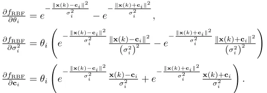
which we refer to as the NLBER algorithm. The step size µ and kernel variance ρ2 should be chosen appropriately to achieve a desired convergence performance, both in terms of convergence speed and steady-state BER misadjustment. For the symmetric RBF detector (9) using the Gaussian RBF function of (11), the derivatives of the RBF detector’s output with respect to the RBF detector’s parameters are given by
∂fRBF ∂θi =e
−x(k)−ci2
σ2i −e−
x(k)+ci2
σ2i ,
∂fRBF ∂σ2
i =θi
e−
x(k)−ci2
σ2
i x(k)−ci2
(σ2
i)2 −
e−
x(k)+ci2
σ2
i x(k)+ci2
(σ2
i)2
,
∂fRBF ∂ci =θi
e−
x(k)−ci2
σ2i x(k)−ci
σ2
i +e
−x(k)+ci2
σ2i x(k)+ci
σ2
i
.
B. The clustering algorithm
Let σˆn2 be an estimated σn2 and set all the RBF variances σi2 = 2ˆσ2n. Further assume that nc = Nsb and set all the RBF weights βi to a same positive value. Then in order for the symmetric RBF detector (9) to realise the Bayesian solution, we have to choose the RBF centresci,1≤i≤Nsb,
TABLE I
NUMBER OF ANTENNA ARRAY ELEMENTS,NUMBER OF USERS SUPPORTED
AND LOCATIONS OF USERS IN TERMS OF ANGLE OF ARRIVAL(AOA).
Example 1: two-element antenna array supporting four users
useri 1 2 3 4
AOAθ 0◦ 20◦ −30◦ −45◦
Example 2: three-element antenna array supporting five users
useri 1 2 3 4 5
AOAθ 0◦ 10◦ −17◦ 15◦ 20◦
appropriately. This task can be achieved by the enhanced κ -means clustering algorithm [16]. Note that unlike in the single-user case, the receiver only has access to b1(k), not b(k), during training, and the following clustering algorithm can be used to update the RBF centres
ci(k) =ci(k−1) +µcMi(ˇx(k))(ˇx(k)−ci(k−1)), (17)
wherexˇ(k) =x(k)ifb1(k) = +1,xˇ(k) =−x(k)ifb1(k) =
−1, andµc is the step size. The membership functionMi(x)
is defined as
Mi(x) =
1, if ¯vix−ci2≤v¯jx−cj2,∀j =i, 0, otherwise,
(18) where¯viis the variation of theith cluster. In order to estimate the associated variationv¯i, the following updating rule is used
¯
vi(k) =µvv¯i(k−1)+(1−µv)Mi(ˇx(k))ˇx(k)−ci(k−1)2, (19) where µv is a constant slightly less than 1.0. The initial variations¯vi(0),∀i, are set to the same small number.
IV. SIMULATION STUDY
Two simulated beamforming systems, as listed in Table I, were used. The array element spacing was half of the wavelength. The simulated narrowband channels were Ai = 1 +j0,1 ≤ i≤M, and the desired user and all the interfering users had equal signal power. Therefore SIRi= 0 dB for2≤i≤M.
-5 -4 -3 -2 -1 0
0 5 10 15 20
log10(Bit Error Rate)
SNR (dB) L-MBER
[image:3.595.47.313.543.636.2]NLBER Bayesian
1e-3 1e-2 1e-1 1
0 500 1000 1500 2000 2500 3000
Bit Error Rate
[image:4.595.84.276.60.203.2]sample Linear MBER NLBER: Esti. BER NLBER: True BER Bayesian
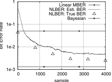
Fig. 2. Learning curve of the NLBER-based RBF detector averaged over 10 runs for the two-element antenna array supporting four users, where SNR=
7dB and the RBF detector hasnc= 8symmetric RBF nodes.
-3 -2 -1 0
0 2 4 6 8 10 12 14
Bit Error Rate
Model Size Linear MBER
[image:4.595.339.532.63.207.2]NLBER Bayesian
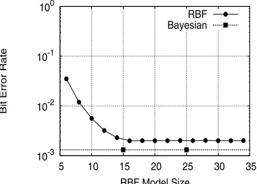
Fig. 3. The influence of the detector’s size on the bit error rate performance of the NLBER-based symmetric RBF detector for the two-element antenna array supporting four users, where SNR= 7dB.
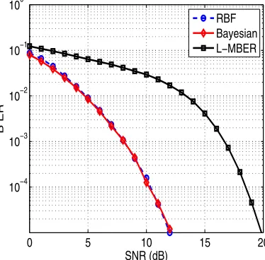
Example 1. Fig. 1 depicts the BERs of both the L-MBER beamformer and the Bayesian detector for the desired user. The size of the Bayesian detector is specified by the number of symmetric signal states Nsb = 8. Given SNR= 7 dB and detector size nc = 8, Fig. 2 shows the learning curve of the NLBER algorithm averaged over 10 runs, where we used the first eight data points as the initial RBF centres ci(0), set the initial RBF weights to θi(0) = 0.1 and the initial RBF variances to σ2i(0) = σ2n, for 1 ≤ i ≤ nc = 8. The step size and kernel variance of the NLBER algorithm (16) were chosen to be µ = 0.4 and ρ2 = 10σ2n. These values were found empirically to be appropriate. The learning curve (dashed curve) was the estimated BER P˜E(w(k)), calculated using (14) with a block size ofK= 400and a kernel variance of ρ2 = σ2n. To check that the estimated BER P˜E(w(k))
gave the correct convergence trend, we also calculated the true BER PE(w(k)) using Monte Carlo simulation for a number of points, shown in Fig. 2 by the triangles. With the same initial conditions, Fig. 3 illustrates the performance of the NLBER-based detector as a function of model size nc. For nc ≥ Nsb the symmetric RBF detector trained by the stochastic NLBER algorithm is capable of closely approaching the optimal Bayesian performance. The BER of the NLBER-based symmetric RBF detector having nc = 8 RBF nodes is depicted in Fig. 1, in comparison to the Bayesian detector.
0 500 1000 1500
0 0.1 0.2 0.3 0.4 0.5 0.6
Training Data Size
Euclidean Distance
[image:4.595.72.273.244.385.2]mu=0.05 mu=0.1 mu=0.2
Fig. 4. Learning curve of the clustering-based RBF detector averaged over 5 runs for the two-element antenna array supporting four users, where SNR=
7dB and the RBF detector hasnc= 8symmetric RBF nodes.
0 5 10 15 20 10−4
10−3 10−2 10−1 100
SNR (dB)
B ER
RBF Bayesian L−MBER
Fig. 5. The desired-user’s bit error rate performance for the two-element antenna array supporting four users at the angular positions of Table I. The clustering-based RBF detector hasnc= 8symmetric RBF nodes.
The clustering-based symmetric RBF detector was next inves-tigated. We used the firstNsbdata points as the initial centres ci(0)and set all the RBF variances to2σ2n. The convergence
of the clustering algorithm (17) was assessed based on the following Euclidean distance metric
ED(k) =
Nsb
i=1
ci(k)−x¯(+)i 2. (20)
[image:4.595.338.525.254.438.2]-5 -4 -3 -2 -1 0
0 5 10 15 20
log10(Bit Error Rate)
SNR (dB) L-MBER
[image:5.595.79.264.56.244.2]NLBER Bayesian
Fig. 6. The desired-user’s bit error rate performance for the three-element antenna array supporting five users at the angular positions of Table I. The NLBER-based RBF detector hasnc= 16symmetric RBF nodes.
1e-3 1e-2 1e-1 1
0 1000 2000 3000 4000
Bit Error Rate
[image:5.595.335.536.58.198.2]sample Linear MBER NLBER: Esti. BER NLBER: True BER Bayesian
Fig. 7. Learning curve of the NLBER-based RBF detector averaged over 10 runs for the three-element antenna array supporting five users, where SNR=
5dB and the RBF detector hasnc= 16symmetric RBF nodes.
Example 2. The BER performance of the two benchmarkers, the L-MBER beamformer and the Bayesian detector, are shown in Fig. 6. The size of the Bayesian detector isNsb= 16. The convergence performance of the NLBER algorithm is characterised in Fig. 7, given SNR= 5 dB and nc = 16. Again, the learning curve of Fig. 7 was averaged over 10 runs, and we used the first 16 data points as the initial RBF centres, set all the initial RBF weights to 0.06 and all the initial RBF variances to9σn2. The two algorithmic parameters of the NLBER algorithm were chosen as step sizeµ= 0.4and kernel variance ρ2= 4σn2. The block size used for estimating the approximated BERP˜E(w(k))wasK= 800with a kernel variance of ρ2 = σ2n. The true BER markers (triangles) in Fig. 7 confirm that the learning curve P˜E(w(k)) correctly indicated the convergence trend and the algorithm achieved convergence after 3000 samples of training. Given SNR= 5dB and the same initial conditions as before, Fig. 8 illustrates the influence of the number of RBF centres nc on the BER performance of the NLBER-based symmetric RBF detector. Usingnc= 16symmetric RBF nodes, the performance of the NLBER-based symmetric RBF detector is compared to those
-3 -2 -1 0
0 5 10 15 20 25 30 35 40
Bit Error Rate
Model Size Linear MBER
[image:5.595.335.536.245.387.2]NLBER Bayesian
Fig. 8. The influence of the detector’s size on the bit error rate performance of the NLBER-based symmetric RBF detector for the three-element antenna array supporting five users, where SNR= 5dB.
0 500 1000 1500 2000 2500 3000 0
0.2 0.4 0.6 0.8 1
Training Data Size
Euclidean Distance
mu=0.1 mu=0.05 mu=0.2
Fig. 9. Learning curve of the clustering-based RBF detector averaged over 5 runs for the three-element antenna array supporting five users, where SNR=
5dB and the RBF detector hasnc= 16symmetric RBF nodes.
of the other two benchmarkers in Fig. 6.
For the clustering-based symmetric RBF detector, again we used the first Nsb data points as the initial centres ci(0) and set all the RBF variances to 2σn2. The convergence of the clustering algorithm (17) averaged over 5 runs was illustrated in Fig. 9 for the three values of the step size µc, where the initial clustering variations ¯vi(0) were again set to 0.01 and the adaptive gain for updating the clustering variations was set toµv= 0.995. The BER performance of the clustering-based symmetric RBF detector is depicted in Fig. 10, in comparison with the two benchmarkers. Finally, Fig. 11 illustrates the influence of the detector’s size on the BER performance of the clustering-based symmetric RBF detector.
V. CONCLUSIONS
[image:5.595.86.279.287.428.2]0 5 10 15 20 10−4
10−3 10−2 10−1 100
SNR (dB)
BER
[image:6.595.73.264.59.246.2]RBF Bayesian L−MBER
Fig. 10. The desired-user’s bit error rate performance for the three-element antenna array supporting five users at the angular positions of Table I. The clustering-based RBF detector hasnc= 16symmetric RBF nodes.
10-3 10-2 10-1 100
5 10 15 20 25 30 35
Bit Error Rate
RBF Model Size RBF Bayesian
Fig. 11. Influence of the detector’s size on the bit error rate performance of the clustering-based symmetric RBF detector for the three-element antenna array supporting five users, where SNR= 5dB.
capable of providing an SNR gain in excess of 8 dB against the powerful linear minimum bit error rate benchmarker, when supporting four users with the aid of two receive antennas or five users employing three receive antenna elements.
ACKNOWLEDGEMENTS
The financial support of the EU under the auspice of the Newcom project is gratefully acknowledged.
REFERENCES
[1] J. Litva and T.K.Y. Lo,Digital Beamforming in Wireless Communica-tions. London: Artech House, 1996.
[2] L. C. Godara, “Applications of antenna arrays to mobile communica-tions, Part II: Beam-forming and direction-of-arrival consideracommunica-tions,”
Proc. IEEE, vol.85, no.8, pp.1193–1245, 1997.
[3] J.H. Winters, “Smart antennas for wireless systems,” IEEE Personal Communications, vol.5, no.1, pp.23–27, 1998.
[4] R. Kohno, “Spatial and temporal communication theory using adaptive antenna array,”IEEE Personal Communications, vol.5, no.1, pp.28–35, 1998.
[5] G.V. Tsoulos, “Smart antennas for mobile communication systems: ben-efits and challenges,”IEE Electronics and Communications J., vol.11, no.2, pp.84–94, 1999.
[6] P. Vandenameele, L. van Der Perre and M. Engels, Space Division Multiple Access for Wireless Local Area Networks. Boston: Kluwer Academic Publishers, 2001.
[7] J.S. Blogh and L. Hanzo,Third Generation Systems and Intelligent Wire-less Networking – Smart Antennas and Adaptive Modulation. Chichester, U.K.: Wiley, 2002.
[8] A. Paulraj, R. Nabar and D. Gore,Introduction to Space-Time Wireless Communications. Cambridge, U.K.: Cambridge University Press, 2003. [9] A.J. Paulraj, D.A. Gore, R.U. Nabar and H. B¨olcskei, “An overview of MIMO communications – A key to gigabit wireless,” Proc. IEEE, vol.92, no.2, pp.198–218, 2004.
[10] D. Tse, and P. Viswanath,Fundamentals of Wireless Communication. Cambridge, U.K.: Cambridge University Press, 2005.
[11] D.N.C. Tse and S.V. Hanly, “Linear multiuser receivers: effective inter-ference, effective bandwidth and user capacity,”IEEE Trans. Information Theory, vol.45, no.2, pp.641–657, 1999.
[12] S. Chen, N.N. Ahmad and L. Hanzo, “Adaptive minimum bit error rate beamforming,”IEEE Trans. Wireless Communications, vol.4, no.2, pp.341–348, 2005.
[13] S. Chen, L. Hanzo, N.N. Ahmad and A. Wolfgang, “Adaptive mini-mum bit error rate beamforming assisted receiver for QPSK wireless communication,”Digital Signal Processing, vol.15, no.6, pp.545–567, 2005.
[14] K. Abend and B.D. Fritchman, “Statistical detection for communication channels with intersymbol interference,” Proc. IEEE, vol.58, no.5, pp.779–785, 1970.
[15] S. Chen, S. McLaughlin, B. Mulgrew and P.M. Grant, “Adaptive Bayesian decision feedback equaliser for dispersive mobile radio chan-nels,”IEEE Trans. Communications, vol.43, no.5, pp.1937–1946, 1995. [16] S. Chen, L. Hanzo and A. Wolfgang, “Nonlinear multi-antenna detection methods,” EURASIP J. Applied Signal Processing, vol.2004, no.9, pp.1225–1237, 2004.
[17] S. Chen and B. Mulgrew, “Overcoming co-channel interference using an adaptive radial basis function equaliser,”Signal Processing, vol.28, no.1, pp.91–107, 1992.
[18] S. Chen, B. Mulgrew and P.M. Grant, “A clustering technique for digital communications channel equalisation using radial basis function networks,”IEEE Trans. Neural Networks, vol.4, no.4, pp.570–579, 1993. [19] A. Wolfgang, S. Chen and L. Hanzo, “Radial basis function network assisted space-time equalisation for dispersive fading environments,”
Electronics Letters, vol.40, no.16, pp.1006–1007, 2004.
[20] F. Albu and D. Martinez, “The application of support vector machines with Gaussian kernels for overcoming co-channel interference,” in
Proc. 9th IEEE Int. Workshop Neural Networks for Signal Processing
(Madison, WI), Aug.23-25, 1999, p.49-57.
[21] D.J. Sebald and J.A. Bucklew, “Support vector machine techniques for nonlinear equalization,”IEEE Trans. Signal Processing, vol.48, no.11, pp.3217–3226, 2000.
[22] S. Chen, A.K. Samingan and L. Hanzo, “Support vector machine multiuser receiver for DS-CDMA signals in multipath channels,”IEEE Trans. Neural Networks, vol.12, no.3, pp.604-611, 2001.
[23] S. Chen, S.R. Gunn and C.J. Harris, “The relevance vector machine technique for channel equalization application,” IEEE Trans. Neural Networks, vol.12, no.6, pp.1529–1532, 2001.
[24] F. P´erez-Cruz, A. Navia-V´azquez, P.L. Alarc´on-Diana and A. Art´es-Rodrguez, “SVC-based equalizer for burst TDMA transmissions,”Signal Processing, vol.81, no.8, pp.1571–1787, 2001.
[25] S. Chen, L. Hanzo and A. Wolfgang, “Kernel-based nonlinear beam-forming construction using orthogonal forward selection with Fisher ratio class separability measure,”IEEE Signal Processing Letters, vol.11, no.5, pp.478–481, 2004.
[26] L.A. Aguirre, R.A.M. Lopes, G.F.V. Amaral and C. Letellier, “Constrain-ing the topology of neural networks to ensure dynamics with symmetry properties,”Physical Review E, vol.69, pp.026701-1–026701-11, 2004. [27] M. Espinoza, J.A.K. Suykens and B. De Moor, “Imposing symmetry in least squares support vector machines regression,” inProc. Joint 44th IEEE Conf. Decision and Control, and the European Control Conf. 2005
(Seville, Spain), Dec.12-15, 2005, pp.5716–5721.
[28] R.O. Duda and P.E. Hart, Pattern Classification and Scene Analysis. New York: Wiley, 1973.
[29] E. Parzen, “On estimation of a probability density function and mode,”
The Annals of Mathematical Statistics, vol.33, pp.1066–1076, 1962. [30] B.W. Silverman, Density Estimation. London, U.K.: Chapman Hall,
1996.
[image:6.595.80.267.287.421.2]