A generalised model for distortion performance analysis of wavelet based watermarking

(1)

wavelet based watermarking

.

White Rose Research Online URL for this paper:

http://eprints.whiterose.ac.uk/76018/

Book Section:

Bhowmik, D. and Abhayaratne, C. (2009) A generalised model for distortion performance

analysis of wavelet based watermarking. In: Kim, H.J., Katzenbeisser, S. and Ho, A. T. S. ,

(eds.) Digital Watermarking. Springer Berlin Heidelberg , pp. 363-378.

https://doi.org/10.1007/978-3-642-04438-0_31

[email protected] https://eprints.whiterose.ac.uk/ Reuse

Unless indicated otherwise, fulltext items are protected by copyright with all rights reserved. The copyright exception in section 29 of the Copyright, Designs and Patents Act 1988 allows the making of a single copy solely for the purpose of non-commercial research or private study within the limits of fair dealing. The publisher or other rights-holder may allow further reproduction and re-use of this version - refer to the White Rose Research Online record for this item. Where records identify the publisher as the copyright holder, users can verify any specific terms of use on the publisher’s website.

Takedown

If you consider content in White Rose Research Online to be in breach of UK law, please notify us by

(2)

Analysis of Wavelet based Watermarking

Deepayan Bhowmik and Charith Abhayaratne

Department of Electronic and Electrical Engineering, University of Sheffield Sheffield S1 3JD, United Kingdom.

{d.bhowmik, c.abhayaratne}@sheffield.ac.uk

Abstract. A model for embedding distortion performance for wavelet based watermarking is presented in this paper. Firstly wavelet based watermarking schemes are generalised into a single common framework. Then a mathematical approach has been made to find the relationship between distortion performance metrics and the watermark embedding parameters. The derived model shows that for wavelet based watermark-ing schemes the sum of energy of the selected wavelet coefficients to be modified is directly proportional to the distortion performance (the mean square error) measured in the pixel domain. The propositions are made using the energy conservation theorem between input signal and trans-form domain coefficients for orthonormal wavelet bases. Such an analysis is useful to choose the wavelet coefficients during watermark embedding procedure and to find suitable input parameters such as wavelet kernel or the choice of subband.

Key words: Watermarking, wavelet transforms, distortion performance.

1 Introduction

With the success of transforms based image/video compression schemes, such as, JPEG, JPEG2000 and MPEG-2, the frequency domain watermarking has received a huge attention. The discrete wavelet transform (DWT) has been widely used as a multi-resolution analysis method in most frequency domain watermarking techniques. [1–11]. Usually the imperceptibility and robustness are considered as two major properties of any watermarking scheme. The im-perceptibility is often measured by evaluating the distortion of the host image.

(3)

DWT (Wv1) Host

Image (I)

Coefficient selection and watermark

embedding

Watermark (W)

IDWT (Wv

1 -1₎

Watermarked

Image (I’) _{(including CA)}Attack

Test Image (J)

DWT (Wv1)

Original Image (I) for non blind detection

Watermark Extraction (Blind / Non-blind) Comparison of

original and extracted watermark

Extracted Watermark (W’) Authentication

Decision

DWT (Wv1) Host

Image (I)

Coefficient selection and watermark

embedding

Watermark (W)

IDWT (Wv

1 -1₎

Watermarked

Image (I’) _{(including CA)}Attack

Test Image (J)

DWT (Wv1)

Original Image (I) for non blind detection

Watermark Extraction (Blind / Non-blind) Comparison of

original and extracted watermark

Extracted Watermark (W’) Authentication

[image:3.595.169.448.115.269.2]

Decision

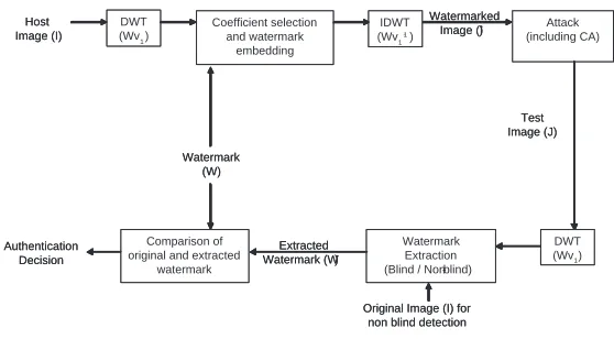
Fig. 1.Block diagram of the generalised functional modules of wavelet based water-marking schemes.

In the distortion performance model first a proposition is made to show the relationship between the noise power in the transform domain and the input signal domain. Then using the above proposition a relationship is established between the distortion performance metrics and the input parameters of a given wavelet based watermarking scheme. The rest of the paper is organised with Sect. 2 presenting the generalisation of embedding schemes. Detailed mathe-matical analysis and the model is presented in Sect. 3 followed by experimental results in Sect. 4. Concluding remarks can be found in Sect. 5.

2 The common framework for wavelet based watermark

embedding

There are many wavelet based watermarking schemes available in the literature. In this context a formal evaluation framework for wavelet based methods is really useful to the watermarking community. It is observed that most of the popu-lar wavelet based watermarking schemes can be dissected in common functional blocks as shown in Fig. 1. In this paper we discuss and present the distortion performance model of wavelet based algorithms and therefore restrict our dis-cussion to the embedding part of the watermarking schemes. In a more general form of the watermarking schemes a forward wavelet transform is applied to the target image. The wavelet coefficients are then modified according to the partic-ular embedding procedure. The modification is done on the selected coefficients in the selected subbands. An inverse wavelet transform which is the same as the forward wavelet kernel is then applied to produce the watermarked image. The basic embedding principle for any wavelet based watermarking algorithm is the same and the modified coefficientC′

m,nat (m, n) position, can be presented as:

C′

(4)

[image:4.595.134.490.140.265.2]

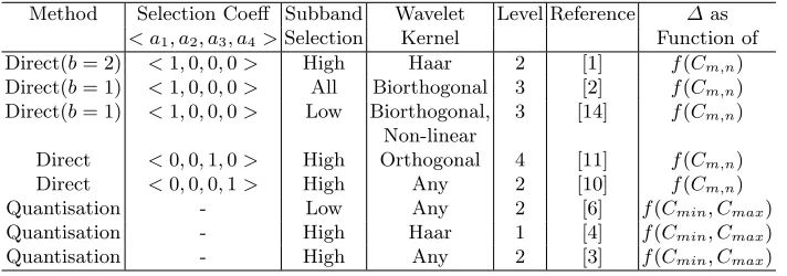
Table 1.Realisation of wavelet based algorithms using different combination of input parameters

Method Selection Coeff Subband Wavelet Level Reference ∆as < a1, a2, a3, a4>Selection Kernel Function of

Direct(b= 2) <1,0,0,0> High Haar 2 [1] f(Cm,n) Direct(b= 1) <1,0,0,0> All Biorthogonal 3 [2] f(Cm,n) Direct(b= 1) <1,0,0,0> Low Biorthogonal, 3 [14] f(Cm,n)

Non-linear

Direct <0,0,1,0> High Orthogonal 4 [11] f(Cm,n) Direct <0,0,0,1> High Any 2 [10] f(Cm,n) Quantisation - Low Any 2 [6] f(Cmin, Cmax) Quantisation - High Haar 1 [4] f(Cmin, Cmax) Quantisation - High Any 2 [3] f(Cmin, Cmax)

where Cm,n is the coefficient to be modified and ∆m,n is the modification due

to watermark embedding. Based on the modification algorithms, the embedding procedures are categorised into two main types of embedding algorithms: direct coefficient modification [1, 2, 7, 10, 11] and quantisation based modification [4, 6, 8, 3].

In the direct coefficient modification schemes, selected coefficients are directly modified based on the following generalised modification value ∆m,n at (m, n)

position:

∆m,n= (a1)α(Cm,n)bWm,n+ (a2)vm,nWm,n+ (a3)βCw+ (a4)Sm,n, (2)

wherea1, a2, a3, a4are the selection coefficients,Cm,nis the coefficient to be

mod-ified,αis the watermark weighting factor,b= 1,2... is the watermark strength parameter,Wm,nis the watermark value,vm,nis the weighting parameter based

on pixel masking in HVS model,β is the weighting parameter in the case of fu-sion based scheme,Cwis the watermark wavelet coefficient andSm,nis any other

value which is normally a function ofCm,n. In most of the algorithms watermark

weighting parametersαandβ are user defined to an optimal value. The water-mark information Wm,n is either generated randomly with a random seed or

taken from a gray scale logo or a binary logo. As mentioned before the weighting parameter and the watermark information are always user defined, hence these are considered as constant parameters in a controlled experimental environment. Other parameters in the modification equation are a function of the wavelet co-efficient Cm,n which depends on the input image and considered as a variable

here. Therefore it is observed that in all the cases the modification value is a direct function of the coefficientCm,n as mentioned in Table 1. This table also

represents the common input parameters used in the embedding procedure and shows how different algorithms can be realised with this generalised framework. Considering a specific case, in this paper we have not chosen HVS model based watermarking scheme as our main focus is on distortion performance analysis which is different from HVS based performance metrics.

(5)

is proposed in these type algorithms. The algorithms change the median value of a local area (typically a 3x1 coefficient window) considering the neighbouring values. The modification value∆m,nis decided based on the quantisation stepδ

(−δ≤∆≤δ) within the range of the selected 3x1 window. Different functions are suggested in the literature to find the value ofδand the functions normally consist of minimum (Cmin) and maximum (Cmax) value of the coefficients in

each selected window. A predefined weighting factor α is often used to deter-mine the value of δ. As ∆ depends on step size δ and α is user defined, the modification value∆ is typically a function ofCmin andCmax in each selected

3x1 window (refer Table 1).

With this common generalised framework we have analysed and proposed a distortion performance model in the next section.

3 Embedding Distortion Performance Analysis

In this section a detailed discussion is carried out on the proposed model. The embedding distortion performance is usually measured by the Mean Square Error (MSE).

Definition 1.TheMean Square Error (MSE)or average noise powerPpin

pixel domain between original imageIand watermarked imageI′ _{is defined by:}

Pp=

1 M N

M−1

X

j=0 N−1

X

i=0

|I(j, i)−I′_{(j, i)}_|2_, ₍₃₎

whereM andN are the image dimension andjandiindicate each pixel position. In order to formulate the model we show the transformation of noise energy from frequency domain to the signal domain using Parseval’s equality.

Definition 2.In theParseval’s Equality, the energy is conserved between an input signal and the transform domain coefficient in the case of an orthonormal filter bank wavelet base [15]. Assuming the input signal x[n] with the length of n∈ Z and the corresponding transformed domain coefficients ofy[k] where k∈Z, according to energy conservation theorem,

kxk2₌_k_y_k2 _. ₍₄₎

Based on these primary definitions we build the model which consists of the following propositions and its proof.

Proposition 1.Sum of the noise power in the transform domain is equal to sum of the noise power in the input signal for orthonormal transforms. If

the input signal noise is defined by∆x[n]and the noise in transform domain is

∆y[k]then

X

n

|∆x[n]|2=X

k

|∆y[k]|2 , (5)

(6)

Proof. The discrete wavelet transform (DWT) can be realised with a filter bank or lifting scheme based factoring. In both cases the wavelet decomposition and the reconstruction can be represented by a polyphase matrix [16]. The in-verse DWT can be defined by a synthesis filter bank using the polyphase matrix M′_{(z) =}³h′e(z)

g′

e(z)

h′

o(z)

g′

o(z)

´

where h′_{(z) represents the low pass filter coefficients and}

g′_{(z) is the high pass filter coefficients and the subscripts} _e_and _o _{denote even}

and odd indexed terms, respectively. Now the transform domain coefficient y can be re-mapped into input signalxas bellow:

³_x

e(z)

xo(z)

´

=³h′e(z)

g′

e(z)

h′

o(z)

g′

o(z)

´ ³_y

e(z)

yo(z)

´

. (6)

Assuming∆yis the noise introduced in wavelet domain and∆xis the modified signal after the inverse transform, we can define the relationship between the noise in the wavelet coefficient and the noise in the modified signal using the following equations. From (6) we can write

³_x

e(z)+∆xe(z)

xo(z)+∆xo(z)

´

=³h′e(z)

g′

e(z)

h′

o(z)

g′

o(z)

´ ³_y

e(z)+∆ye(z)

yo(z)+∆yo(z)

´

. (7)

From (7) using theLinearity property of theZtransform of the filter coefficients and signals in the polyphase matrix we can get,

xe(z) +∆xe(z) =h′e(z)(ye(z) +∆ye(z))

+h′

o(z)(yo(z) +∆yo(z)),

h′

e(z)ye(z) +h′o(z)yo(z) +∆xe(z) =h′e(z)ye(z) +h′e(z)∆ye(z)

+h′

o(z)yo(z) +h′o(z)∆yo(z),

∆xe(z) =h′e(z)∆ye(z) +h′o(z)∆yo(z). (8)

Similarly∆xo(z) can be obtained and written as

∆xo(z) =g′e(z)∆ye(z) +go′(z)∆yo(z). (9)

Combining (8) and (9), finally we can write the polyphase matrix form of the noise in the output signal:

³_∆x

e(z)

∆xo(z)

´

=³h′e(z)

g′

e(z)

h′

o(z)

g′

o(z)

´ ³_∆y

e(z)

∆yo(z)

´

. (10)

Recalling the Parseval’s energy conservation theorem as stated inDefinition 2., from (10) we can conclude that

X

|∆xe|2+

X

|∆xo|2 =

X

|∆ye|2+

X

|∆yo|2 ,

X

n

|∆x[n]|2 =X

k

|∆y[k]|2 . (11)

(7)

Using the generalised framework, theProposition 1 can be applied to build the relationship between the modification energy in the coefficient domain to embed the watermark and the distortion performance metrics. In this model we made propositions for two different categories of embedding schemes, discussed in previous section.

Proposition 2.In a wavelet based watermarking scheme, the mean square error (MSE) of the watermarked image is directly proportional to the sum of the energy of the modification values of the selected wavelet coefficients. The modification value itself is a function of the wavelet coefficients and therefore we propose two different cases based on the categorisation.

Case A.For the direct modification embedding method the modification is a function of the selected coefficient to be watermarked and the relationship between

MSE (Pp) and the selected coefficient (Cm,n) is expressed as:

Pp∝

X

|f(Cm,n)|2. (12)

Case B.For the quantisation based method the modification is a function of the neighbouring wavelet coefficients of the selected median coefficient to be

watermarked and the relationship between MSE (Pp) and the wavelet coefficients

Cmin andCmax is expressed as:

Pp∝

X

|f(Cmin, Cmax)|2 . (13)

Proof.In a wavelet based watermark embedding scheme the watermark

informa-tion is inserted by modifying the wavelet coefficients. This watermark inserinforma-tion can be considered as introducing noise in the transform domain. Hence the sum of the energy of the modification value due to watermark embedding in the wavelet domain is equal to the sum of the noise energy in the transform domain as stated inProposition 1.From (1) and (5), the energy sum of the modification value∆m,ncan be defined as:

X

m,n

|∆m,n|2=

X

k

|∆y[k]|2 . (14)

Similarly, the pixel domain distortion performance metrics which is represented by MSE is considered as the noise error created in the signal due to the noise in wavelet domain. Therefore, the sum of the noise energy in the input signal is equal to the sum of the noise error energyPp in the pixel domain:

Pp.(M N) =

X

n

|∆x[n]|2 _, ₍₁₅₎

where M and N are the image dimensions. Now the relationship between the distortion performance metrics MSE of the watermarked image and the coef-ficient modification value which is normally a function of the selected wavelet coefficients can be decided using theProposition 1.Thus from (14) and (15) we can write:

(8)

where M and N are the image dimensions. Hence for any watermarked image, the average noise power Pp is proportional to the sum of the energy of the

modification values of the selected wavelet coefficients:

Pp∝Pm,n|∆m,n|2. (17)

Now with the help of the categorisation in the generalised form of the popular wavelet based watermarking schemes as discussed in Sect. 2, a relationship is established between the error energy of the watermarked image and the selected wavelet coefficient energy of the host image. For a direct modification based algorithm, the mean square errorPp is directly proportional to the sum of the

energy of the modification value∆which is a function of wavelet coefficient value as stated below:

Pp∝

X

|f(Cm,n)|2. (18)

Similarly for the quantisation based method the mean square error depends on the neighbouring wavelet coefficient values. In this case the modification energy

|∆m,n|2 hold an inequality due the modification range−δ≤∆m,n≤δ:

|∆m,n|2≤ |δ|2 . (19)

Therefore the upper bound of the mean square errorPp is defined by:

Pp∝

X

|f(Cmin, Cmax)|2 . (20)

¥

3.1 An Example of Direct Modification

Considering a specific case of the direct modification algorithm in [2] the modifi-cation value∆is a direct function of wavelet coefficient (∆m,n=αCm,nW m, n).

Hence (18) can be modified and the MSEPp can be expressed as:

Pp∝ l

X

k=1

|C(k)|2 _, ₍₂₁₎

whereC(k) is the selected coefficients to be watermarked andlis the number of such selected coefficients.

3.2 An Example of Quantisation based Method

In an intra subband based quantisation method suggested in [6], the quantisation stepδis defined as:

δ=αCmax+Cmin

2 , (22)

whereαis the user defined weighting factor. As the modification value∆depends onδ, with reference to (20), the relationship between the maximum limit of MSE Pp and wavelet energy is defined by the following equation:

Pp∝

X

k

(C(k)max+C(k)min)2 , (23)

where C(k)max and C(k)min are the neighbourhood coefficients of the median

(9)

Table 2.Correlation coefficient values between sum of energy and the MSE for different wavelet kernel in various subbands.

Direct modification Intra Subband Based

Haar D-4 D-6 D-8 D-10 D-16 Haar D-4 D-6 D-8 D-10 D-16 LL3 0.99 0.99 0.99 0.99 0.99 0.99 0.80 0.84 0.87 0.88 0.86 0.89 LH3 0.99 0.99 0.99 0.99 0.99 0.99 0.99 0.99 0.99 0.99 0.99 0.99 HL3 0.99 0.99 0.99 0.99 0.99 0.99 0.93 0.96 0.95 0.96 0.97 0.99 HH3 0.99 0.99 0.99 0.99 0.99 0.99 0.99 0.99 0.99 0.99 0.99 0.99 LH2 0.99 0.99 0.99 0.99 0.99 0.99 0.99 0.99 0.99 0.99 0.99 0.99 HL2 0.99 0.99 0.99 0.99 0.99 0.99 0.99 0.99 0.99 0.99 0.99 0.99 HH2 0.99 0.99 0.99 0.99 0.99 0.99 0.99 0.99 0.99 0.99 0.99 0.99 LH1 0.99 0.99 0.99 0.99 0.99 0.99 0.99 0.99 0.99 0.99 0.99 0.99 HL1 0.99 0.99 0.99 0.99 0.99 0.99 0.97 0.98 0.99 0.98 0.98 0.99 HH1 0.99 0.99 0.99 0.99 0.99 0.99 0.99 0.99 0.99 0.99 0.99 0.99

4 Experimental Simulations

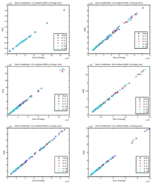
The propositions made in the previous section are verified in the experimental simulations. The sum of the energy of the selected wavelet coefficients and the MSE of the watermarked image have been calculated for 30 different images with a combination of different input parameters. As the wavelet coefficients varies greatly in different subbands we have considered the performances of all subbands separately after a 3 level wavelet decomposition. Also a set of dif-ferent wavelet kernels having various filter lengths are selected to perform the simulations. We simulated and studied the performance of different wavelet ker-nels such as Haar, Daubechies-4 (D-4), Daubechies-6 (D-6), Daubechies-8 (D-8), Daubechies-10 (D-10) and Daubechies-16 (D-16) in order to verify our proposed model. Two different sets of results are obtained and displayed to verify the effects of different input parameters which are responsible for embedding distor-tion performance. These two sets of experimental arrangements and resulting plots are discussed separately as follows:

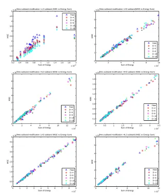
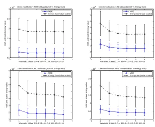
– In the experimentSet 1, the sum of energy of the selected wavelet coefficients to be modified and MSE of the watermarked image have been calculated using the same α and the same binary watermark logo for each selected method. We have used various wavelet kernels and observed the results for each selected subbands. The correlation between MSE and the energy sum is displayed in Fig. 2 and Fig. 3 for direct modification and intra subband based embedding, respectively. The correlation coefficients are also calculated and presented in Table 2.

(10)

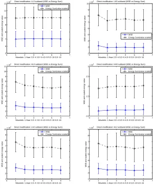
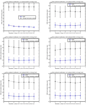
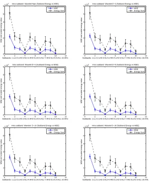
– In the experimentSet 2, the performance for different subbands are plotted for each wavelet kernel in a similar fashion as mentioned in experimentSet 1

in order to observe the trend. The direct modification results are shown in Fig. 7 and the intra subband modification methods are shown in Fig. 8. As earlier, a 95% confidence interval is considered which is denoted by the error bars.

2 4 6 8 10 12 14 16

x 109

0.2 0.4 0.6 0.8 1 1.2 1.4 1.6 1.8 2x 10

9 Direct modification: LL3 subband (MSE vs Energy Sum)

Sum of Energy

MSE Haar D−4 D−6 D−8 D−10 D−16

0 1 2 3 4 5 6 7 8

x 107

0 1 2 3 4 5 6 7 8 9x 10

6 Direct modification: LH3 subband (MSE vs Energy Sum)

Sum of Energy

0 2 4 6 8 10 12

x 107

0 2 4 6 8 10 12 14x 10

6 Direct modification: HL3 subband (MSE vs Energy Sum)

Sum of Energy

0 0.5 1 1.5 2 2.5

x 107

0 0.5 1 1.5 2 2.5

3x 10

6 Direct modification: HH3 subband (MSE vs Energy Sum)

Sum of Energy

0 1 2 3 4 5 6 7

x 107 0 1 2 3 4 5 6 7 8x 10

Sum of Energy

0 2 4 6 8 10

x 107 0 2 4 6 8 10 12x 10

Sum of Energy

[image:10.595.153.457.219.586.2]

(11)

0.2 0.4 0.6 0.8 1 1.2 1.4 1.6 1.8 2 x 1010

0 0.5 1 1.5 2 2.5 3 3.5 4 4.5 5x 10

4Intra subband modification: LL3 subband (MSE vs Energy Sum)

Sum of Energy

0 2 4 6 8 10

x 107

0 1 2 3 4 5 6x 10

5Intra subband modification: LH3 subband(MSE vs Energy Sum)

Sum of Energy

0 2 4 6 8 10 12 14

x 107

0 1 2 3 4 5 6 7x 10

5Intra subband modification: HL3 subband (MSE vs Energy Sum)

Sum of Energy

0 0.5 1 1.5 2 2.5 3 3.5

x 107

0 0.2 0.4 0.6 0.8 1 1.2 1.4 1.6 1.8

2x 10

5

Intra subband modification: HH3 subband (MSE vs Energy Sum)

Sum of Energy

0 1 2 3 4 5 6 7 8 9

x 107 0 0.5 1 1.5 2 2.5 3 3.5 4 4.5 5x 10

5Intra subband modification: LH2 subband (MSE vs Energy Sum)

Sum of Energy

0 2 4 6 8 10 12

x 107 0 1 2 3 4 5 6x 10

Sum of Energy

[image:11.595.143.457.103.484.2]

Fig. 3. Watermark embedding (Intra subband based) performance correlation plot: MSE vs. sum of energy, in different subband for individual images. Six wavelet kernels used here such as 1. Haar, 2. D-4, 3. D-6, 4. D-8, 5. D-10 and 6. D-16, respectively.

The simulation results show a strong correlation between MSE of the wa-termarked image and the energy sum of the selected wavelet coefficients to be modified. It is observed that for a direct modification, the correlation coefficient value is more than 0.97 and more than 0.80 in the case of intra subband based modification, for different wavelet kernels and various selected subbands. On the other hand, a similar graph patterns are observed in Fig. 4, Fig. 5, Fig. 6, Fig. 7 and Fig. 8, which show the proportionality trend between MSE and the energy sum as proposed in the model.

(12)

0 1 2 3 4 5 6 7 5

6 7 8 9 10 11 12x 10

8 Direct modification: LL3 subband (MSE vs Energy Sum)

Wavelets: 1.Haar 2.D−4 3.D−6 4.D−8 5.D−10 6.D−16

MSE and scaled energy value

MSE

Energy Sum(value scaled)

0 1 2 3 4 5 6 7

2 3 4 5 6 7 8 9 10x 10

MSE

0 1 2 3 4 5 6 7

1 2 3 4 5 6 7 8 9 10 11x 10

MSE

0 1 2 3 4 5 6 7

0.5 1 1.5 2 2.5

3x 10

MSE

0 1 2 3 4 5 6 7

1 2 3 4 5 6 7 8 9 10x 10

MSE

0 1 2 3 4 5 6 7

1 2 3 4 5 6 7 8 9x 10

MSE

[image:12.595.155.454.118.485.2]

Fig. 4.Watermark embedding (Direct Modification) performance graph for different subbands. Six different wavelet kernels used here such as 1. Haar, 2. D-4, 3. D-6, 4. D-8, 5. D-10 and 6. D-16, respectively. Subbands are shown left to right and top to bottom: LL3, LH3, HL3, HH3, LH2 and HL2, respectively.

5 Conclusions

(13)

veri-0 1 2 3 4 5 6 7 0.5

1 1.5 2 2.5 3x 10

MSE

0 1 2 3 4 5 6 7

0 1 2 3 4 5 6 7 8x 10

MSE

0 1 2 3 4 5 6 7

1 2 3 4 5 6 7 8x 10

MSE

0 1 2 3 4 5 6 7

0 0.5 1 1.5 2 2.5

3x 10

MSE

[image:13.595.148.456.107.360.2]

Fig. 5. Watermark embedding (Direct modification) performance graph for different subbands. Six different wavelet kernels used here such as 1. Haar, 2. D-4, 3. D-6, 4. D-8, 5. D-10 and 6. D-16, respectively. Subbands are shown left to right and top to bottom: HH2, LH1, HL1, HH1.

fied the model by evaluating the embedding distortion performance for different choices of wavelet kernels, subbands and the coefficient selections used in wavelet based watermark embedding. The experimental simulation successfully verified the proposed model.

Acknowledgments: This work is funded by BP-EPSRC Dorothy Hodgkin

postgraduate award.

References

1. Xia, X., Boncelet, C.G., Arce, G.R.: Wavelet transform based watermark for digital images. Optic Express3(12) (Dec. 1998) 497–511

2. Kim, J.R., Moon, Y.S.: A robust wavelet-based digital watermarking using level-adaptive thresholding. In: Proc. IEEE ICIP. Volume 2. (1999) 226–230

3. Huo, F., Gao, X.: A wavelet based image watermarking scheme. In: Proc. IEEE ICIP. (Oct. 2006) 2573–2576

(14)

0 1 2 3 4 5 6 7 0

1 2 3 4 5 6 7 8 9x 10

4Intra subband modification: LL3 subband (MSE vs Energy Sum)

MSE

0 1 2 3 4 5 6 7

1 1.5 2 2.5 3 3.5 4 4.5 5 5.5

6x 10

MSE

0 1 2 3 4 5 6 7

0.5 1 1.5 2 2.5 3 3.5 4 4.5 5x 10

MSE

0 1 2 3 4 5 6 7

0.2 0.4 0.6 0.8 1 1.2 1.4 1.6 1.8x 10

5Intra subband modification: HH3 subband (MSE vs Energy Sum)

MSE

0 1 2 3 4 5 6 7

1 1.5 2 2.5 3 3.5 4 4.5 5 5.5x 10

MSE

0 1 2 3 4 5 6 7

0.5 1 1.5 2 2.5 3 3.5 4 4.5x 10

MSE

[image:14.595.155.455.115.483.2]

Fig. 6. Watermark embedding (Intra subband modification) performance graph for different subbands. Six different wavelet kernels used here such as 1. Haar, 2. D-4, 3. D-6, 4. D-8, 5. D-10 and 6. D-16, respectively. Subbands are shown left to right and top to bottom: LL3, LH3, HL3, HH3, LH2 and HL2, respectively.

5. Wang, H.J., Su, P.C., Kuo, C.C.J.: Wavelet-based digital image watermarking. Optics Express3(Dec. 1998) 491–497

6. Xie, L., Arce, G.R.: Joint wavelet compression and authentication watermarking. In: Proc. IEEE ICIP. Volume 2. (1998) 427–431

7. Barni, M., Bartolini, F., Piva, A.: Improved wavelet-based watermarking through pixel-wise masking. IEEE Trans. Image Processing10(5) (May 2001) 783–791 8. Jin, C., Peng, J.: A robust wavelet-based blind digital watermarking algorithm.

Information Technology Journal5(2) (2006) 358–363

(15)

0 2 4 6 8 10 12 0

0.5 1 1.5 2 2.5x 10

7 Direct Mod.: Wavelet:Haar (Subband Energy vs MSE)

Subbands: 1.LL3 2.LH3 3.HL3 4.HH3 5.LH2 6.HL2 7.HH2 8.LH1 9.HL1 10.HH1

MSE Energy Sum

0 2 4 6 8 10 12

0 0.5 1 1.5 2 2.5x 10

7 Direct Mod.: Wavelet:D−4 (Subband Energy vs MSE)

MSE Energy Sum

0 2 4 6 8 10 12

0 0.5 1 1.5 2 2.5x 10

MSE Energy Sum

0 2 4 6 8 10 12

0 0.5 1 1.5 2 2.5x 10

MSE Energy Sum

0 2 4 6 8 10 12

0 0.5 1 1.5 2 2.5x 10

7 Direct Mod.: Wavelet: D−10 (Subband Energy vs MSE)

MSE and scaled energy value)

MSE Energy Sum

0 2 4 6 8 10 12

0 0.5 1 1.5 2 2.5x 10

[image:15.595.148.459.104.481.2]

MSE Energy Sum

Fig. 7. Watermark embedding (Direct Modification) performance graph for various wavelets in different subband. Wavelet kernels are shown left to right and top to bottom: Haar, D-4, D-6, D-8, D-10 and D-16, respectively.

technologies (PDCAT 2005). (Dec. 2005) 1058–1062

10. Feng, X.C., Yang, Y.: A New Watermarking Method Based on DWT. Lecture Notes in Computer Science3802(2005) 1122–1126

11. Kundur, D., Hatzinakos, D.: Toward robust logo watermarking using multiresolu-tion image fusion principles. IEEE Trans. Multimedia6(1) (Feb. 2004) 185–198 12. Ejima, M., Miyazaki, A.: On the evaluation of performance of digital watermarking

in the frequency domain. In: Proc. IEEE ICIP. Volume 2. (Oct. 2001) 546–549 13. Bhowmik, D., Abhayaratne, C.: Evaluation of watermark robustness to JPEG2000

(16)

0 2 4 6 8 10 12 0

1 2 3 4 5 6x 10

4 Intra subband: Wavelet:Haar (Subband Energy vs MSE)

MSE Energy Sum

0 2 4 6 8 10 12

0 1 2 3 4 5 6x 10

4 Intra subband: Wavelet:D−4 (Subband Energy vs MSE)

MSE Energy Sum

0 2 4 6 8 10 12

0 1 2 3 4 5 6x 10

MSE Energy Sum

0 2 4 6 8 10 12

0 1 2 3 4 5 6x 10

MSE Energy Sum

0 2 4 6 8 10 12

0 1 2 3 4 5 6x 10

4 Intra subband: Wavelet: D−10 (Subband Energy vs MSE)

MSE Energy Sum

0 2 4 6 8 10 12

0 1 2 3 4 5 6x 10

[image:16.595.159.459.113.482.2]

MSE Energy Sum

Fig. 8. Watermark embedding (Intra subband modification) performance graph for various wavelets in different subband. Wavelet kernels are shown left to right and top to bottom: Haar, D-4, D-6, D-8, D-10 and D-16, respectively.

14. Zhang, Z., Mo, Y.L.: Embedding strategy of image watermarking in wavelet trans-form domain. In: Proc. Image Compression and Encryption Technologies. Volume 4551., SPIE (2001) 127–131

15. Vetterli, M., Kovaˇcevic, J.: Wavelets and subband coding. Prentice-Hall, Inc., Upper Saddle River, NJ, USA (1995)