This is a repository copy of
Reservation Wages, Expected wages and the duration of
Unemployment: evidence from British Panel data
.
White Rose Research Online URL for this paper:
http://eprints.whiterose.ac.uk/9988/
Monograph:
Brown, S. and Taylor, K. (2009) Reservation Wages, Expected wages and the duration of
Unemployment: evidence from British Panel data. Working Paper. Department of
Economics, University of Sheffield ISSN 1749-8368
Sheffield Economic Research Paper Series 2009001
eprints@whiterose.ac.uk https://eprints.whiterose.ac.uk/ Reuse
Unless indicated otherwise, fulltext items are protected by copyright with all rights reserved. The copyright exception in section 29 of the Copyright, Designs and Patents Act 1988 allows the making of a single copy solely for the purpose of non-commercial research or private study within the limits of fair dealing. The publisher or other rights-holder may allow further reproduction and re-use of this version - refer to the White Rose Research Online record for this item. Where records identify the publisher as the copyright holder, users can verify any specific terms of use on the publisher’s website.
Takedown
If you consider content in White Rose Research Online to be in breach of UK law, please notify us by
Sheffield Economic Research Paper Series
SERP Number: 2009001
ISSN 1749-8368
Sarah Brown and Karl Taylor
*Reservation Wages, Expected wages and the duration of Unemployment:
evidence from British Panel data
January 2009
* Department of Economics University of Sheffield 9 Mappin Street Sheffield S1 4DT
United Kingdom
Abstract:
In this paper we analyse the role of wage expectations in an empirical model of incomplete spells of unemployment and reservation wages. To be specific, we model the duration of unemployment, reservation wages and expected wages simultaneously for a sample of individuals who are not in work, where wage expectations are identified via an exogenous policy shock based upon the introduction of Working Family Tax Credits (WFTC) in the UK. The results from the empirical analysis, which is based on the British Household Panel Survey, suggest that WFTC eligibility served to increase expected wages and that expected wages are positively associated with reservation wages. In addition, incorporating wage expectations into the econometric framework was found to influence the magnitude of the key elasticities: namely the elasticity of unemployment duration with respect to the reservation wage and the elasticity of the reservation wage with respect to unemployment duration.
Keywords: Expected Wages; Reservation Wages; and Unemployment Duration.
JEL codes: J13; J24; J64
Acknowledgements:
We are grateful to the ESRCfor financial support under grant number RES-000-22-2004 and to the Data Archive, University of Essex, for supplying the British Household Panel Surveys,
I. Introduction and Background
The reservation wage, the lowest wage at which an individual is willing to work, plays a key
role in labour market theory. In particular, the reservation wage plays an important role in
theoretical models of job search, labour supply and labour market participation (see, for
example, Mortensen, 1986, Mortensen and Pissarides, 1999, and Pissarides, 2000). An
extensive empirical literature exists, which has explored the implications of reservation wage
setting at the individual level focusing on the relationship between reservation wages and the
duration of unemployment, an area of particular interest to policy-makers, with seminal
contributions made by Lancaster and Chesher (1983, 1984) and Jones (1988).
The empirical evidence has supported a positive relationship between reservation
wages and the duration of unemployment as predicted by optimal job search theory, i.e. high
reservation wages are associated with longer spells of unemployment. It is important to
acknowledge that there have been a number of issues, which have complicated the empirical
analysis in this area. For example, there is a shortage of data sets which include information
relating to reservation wages at the individual level, with early studies based on the offered
wages of individuals who have been unemployed at some point in time (see Kiefer and
Neumann, 1979). Furthermore, reservation wages and the duration of unemployment are
arguably jointly determined: reservation wages influence the probability of exiting
unemployment and reservation wages are influenced by the length of the spell of
unemployment.
Two main approaches have been adopted in the empirical literature to explore the
relationship between reservation wages and the duration of unemployment. Lancaster and
Chesher (1983) pioneered an approach whereby, rather than estimating the response of
reservation wages to the unemployment rate, they calculate the elasticity of the reservation
approach has been recently used by Blackaby et al. (2007) to explore the reservation wages of
‘economically inactive’ rather than unemployed individuals and by Addison et al. (2009) to
explore reservation wage and unemployment duration elasticities across a number of
European labour markets. The second approach which has been used extensively in the
existing literature to explore the relationship between reservation wages and the duration of
unemployment is the instrumental variables (IV) approach introduced by Jones (1988), which
we adopt in order to allow for the joint determination of the reservation wage and the
duration of unemployment.
In the existing empirical literature, it is apparent that, although the role of expected
wages has been acknowledged, it has not been explicitly incorporated into the econometric
analysis. For example, Lancaster and Chesher (1983) regard reservation wages, expected
wages and the duration of unemployment as three jointly determined variables. However, in
the context of their non parametric approach they do not calculate the effect of expected
wages on reservation wages. In contrast, we aim to analyse the effect of expected wages on
reservation wages and how including the expected wage into the framework influences the
relationship between the reservation wage and the duration of unemployment. Thus, we
expand the framework introduced by Jones (1988) by jointly modelling these three variables
using individual level data drawn from the British Household Panel Survey (BHPS).
The inclusion of the expected wage within this framework is an important
contribution to this area since, although its potential role has been alluded to in the existing
empirical literature on reservation wages, its role on reservation wage setting has not been the
focus of empirical scrutiny. This is not surprising, however, since although individuals’
expectations play a central role in many areas of economic theory, microeconometric
evidence of their causes and effects is relatively sparse. The work that does exist is
predominately focused on financial expectations, exploring the motivation behind, for
and van Soest, 1999 and Souleles, 2004). The absence of a wider research programme is
perhaps reflective of both a shortage of relevant data and scepticism amongst economists
over the use of subjective information on expectations drawn from surveys (see Manski,
2004).
In order to contribute to the empirical literature on labour market expectations, we
explore how a change in labour market policy in the UK influences the expected wages of
individuals who are not in work. To be specific, we analyse how eligibility for Working
Family Tax Credits (WFTC), which replaced and expanded the generosity of Family Credits
in 1999, influences the expected wages of the unemployed. According to Brewer et al.
(2006), the introduction of the WFTC in 1999 almost doubled the generosity of the previous
in-work benefits associated with the Family Credits scheme, thereby aiming to encourage
individuals currently on benefit into employment. Thus, the influence of the introduction of
the WFTC on expected wages and the subsequent effects on reservation wages and the
duration of unemployment present a potentially important contribution to the empirical
literature in this area, which should be of particular interest to policy makers.
II. Data
Our empirical analysis is based on panel data drawn from the BHPS, which is a random
sample survey, carried out by the Institute for Social and Economic Research, of each adult
member from a nationally representative sample of more than 5,000 private households
(yielding approximately 10,000 individual interviews). For wave one, interviews were
conducted during the autumn of 1991. The same individuals are re-interviewed in successive
waves. Given the availability of detailed information on job search in the BHPS, we focus on
the time period 1996 to 2002. In addition, the start of our period of study coincides with the
introduction of the Job Seekers Allowance (JSA) in the UK, which tightened the job search
requirements for benefit eligibility. As detailed by Manning (2005), all claimants had to sign
to work; and the steps taken to identify and apply for jobs. In 2003, Working Tax Credit and
Child Tax Credit replaced WFTC, hence our sample ends in 2002.
The defining feature of the BHPS for our empirical study is that it contains detailed
information on reservation wages, expected wages and the duration of unemployment at the
individual level. To be specific, if the respondent ‘is not currently working but has looked for
work or has not looked for work in last four weeks but would like a job’, he/she is asked to
specify: ‘What is the lowest weekly take home pay you would consider accepting for a job?’
This series of questions is asked in all waves of the BHPS. Individuals who answer the
question regarding lowest pay are then asked: ‘About how many hours in a week would you
expect to have to work for that pay?’ This enables us to construct the hourly reservation
wage.1 Turning to expected wages, in all waves of the BHPS, job seekers were asked: ‘About
how many hours in a week do you think you would be able to work?’ Such individuals are
then explicitly asked about their expected wage: ‘What weekly take-home pay would you
expect to get (for that)?’ Hence, we are also able to construct the hourly expected wage. The
duration of unemployment is measured as the length of time in the current labour market
spell (measured in days), i.e. whether employed, self employed or not in work.
Our sample comprises those individuals not in employment or self-employment. The
data set is unbalanced with 3,034 observations for the seven years where, on average,
individuals are in the panel for two years. The sample includes individuals of working age
(16-65) who satisfy the rationality restriction of Lancaster and Chesher (1983), i.e. that
unemployment benefit income is less than or equal to the reservation wage, which in turn is
less than or equal to the expected wage.2 Out of the sample of individuals who are currently
1
Given the reference to ‘take home pay’ in the question, it seems reasonable to assume that respondents would refer to the net (i.e. after tax) wage. It should be acknowledged that Hofler and Murphy (1994), who use stochastic frontier techniques to estimate reservation wages for a sample of employed individuals, argue that the reservation wage declared by individuals in surveys may be measured inaccurately. For example, individuals may not be well-informed enough to provide an accurate answer or it may be difficult to factor in non-wage characteristics of jobs, which may entice individuals into accepting job offers.
2
not working and who state that they havelooked for work or have not looked for work in the
last four weeks but would like a job, 61.96% are typically classified as ‘economically
inactive’.3 We include these individuals in the sample if they report a reservation wage, since
in so doing they are arguably signaling their attachment to the labour market. Such an
approach is in accordance with recent contributions in the labour economics literature, which
recognise that the distinction between the unemployed and inactive may not necessarily be as
clear-cut as previously assumed in the labour economics literature and that some of those
traditionally labelled as inactive do actually want to work (see, for example, Schweitzer,
2003, and Blackaby et al., 2007).4
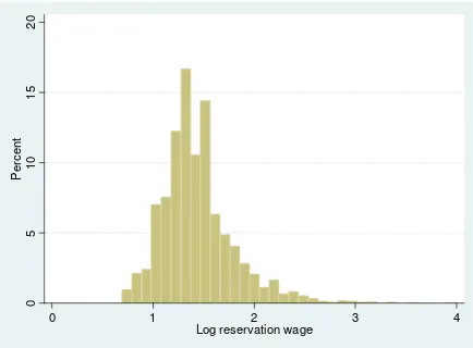
The distribution of the natural logarithm of the reservation wage is presented in
Figure 1, where the mean log hourly reservation wage is 1.438, i.e. an hourly reservation
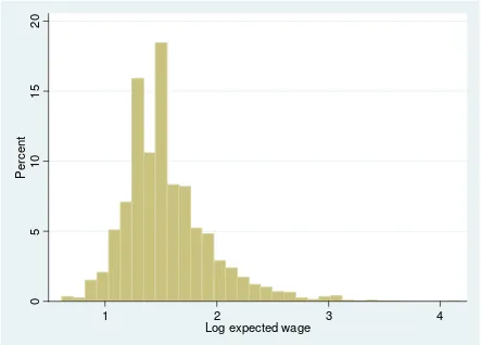
wage of approximately £4.21. Similarly, the distribution of the natural logarithm of the
expected wage is shown in Figure 2, where the mean log expected wage is 1.549, i.e. an
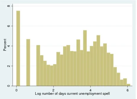
hourly expected wage of approximately £4.71. Figure 3 shows the distribution of the natural
logarithm of the number of days not in work, where the mean is 3.041, i.e. around 21 days,
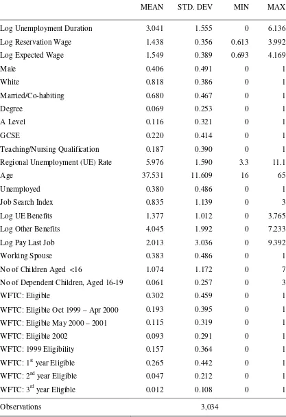
the minimum is 1 day and the maximum just over 1 year and 3 months. Full summary
statistics are presented in Table 1A where all monetary values have been deflated to 1991
prices. The average age in the sample is 38 years old and 22% of individuals in the sample
have a GCSE level qualification as their highest level of educational attainment. Most
individuals who are not in work have undertaken at least one type of job search, which is
consistent with JSA requirements.5
3
The ‘economically inactive’ group includes: individuals involved in family care; full time students; the long term sick or disabled; and individuals involved in government training. In the BHPS, 1996 to 2002, 80.1% of those typically classified as ‘economically’ inactive do not specify a reservation wage, with the remaining 19.9%, who do specify a reservation wage, being included in our estimation sample. Amongst the latter, the ‘family care’ group dominates.
4
Throughout the paper, the term unemployment duration describes the duration of being out of work for both groups, i.e. the unemployed and the ‘economically’ inactive.
5
III. Reservation Wages and the Duration of Unemployment
Methodology
In the BHPS, the duration of unemployment reflects a current rather than completed spell of
unemployment as recorded at the interview date. Hence, by definition, when the reservation
wage information is recorded, there are no exits from unemployment into employment, i.e.
information on reservation wages is only reported for those who are not in work. In this
context, Jones (1988) proposed the following structural model, i.e. a system of two
simultaneous equations, estimated by instrumental variables on elapsed unemployment
duration:
( )
( )
( )
( )
1it 1 2it 2 log log log log it it it it it it t rw rw tβ γ ε
φ λ ε
= + +
= + +
X
X (1)
where i and t denote the individual and time period respectively, log
( )
t is the log duration ofthe number of days not being in work, log
( )
rw is the log hourly reservation wage, X1 and2
X are vectors of variables which influence unemployment duration and the reservation
wage respectively, β and φ are parameters to be estimated and capture the influence of the
explanatory variables on the reservation wage and unemployment duration respectively, γ
and λ measure the elasticity of unemployment duration with respect to the reservation wage
and the elasticity of the reservation wage with respect to unemployment duration, and the ε’s
are random error terms. In accordance with the existing literature, we include the following
variables in both X1 and X2: gender; ethnicity; marital status; highest level of educational
attainment; the regional unemployment rate (see Jones, 1988, and Haurin and Sridhar,
2003)6; a quadratic in age; whether the individual is currently unemployed rather than
‘economically inactive’; and the index of job search intensity. To identify the unemployment
6
duration equation, the vector X2 also includes: following Jones (1988), log unemployment
benefits, which arguably influence job search costs; the log of the sum of all other types of
benefit income; following Kiefer and Neumann (1979) and Hui (1991), the log of pay in last
job; having a working spouse; the number of children under 16; and the number of dependent
children aged 16 to 19. Our set of over-identifying instruments follows the existing literature
and, in particular, is consistent with Lancaster (1985). In both the unemployment duration
and reservation wage equations, we also include a set of region, year and month of interview
binary controls.
Due to the panel nature of the data in order to allow for individual time invariant, i.e.
fixed effects, we include a vector of individual level mean characteristics of time varying
covariates for control variables in Z1i,Z1i ⊃
{
X1i, log( )
rw}
, and Z2i, Z2i ⊃{
X2i, log( )
t}
,for the unemployment duration and reservation wage equations, respectively. This enables
the parameters β, γ, φ and λ to be considered as an approximation to a fixed effects
estimator. Hence, following Mundlak (1978), equation (1) is modified as follows:
( )
( )
( )
( )
1it 1i 1
2it 2i 2
log log log log it it it it it it t rw rw t
β γ π ε
φ λ θ ε
= + + +
= + + +
X Z
X Z (2)
The Mundlak transformation to allow for fixed effects has been adopted in a range of labour
market applications, see, for example, Korkeamäki and Kyyrä (1996), Barth (1997) and,
more recently, Kirby and Riley (2008).
Results
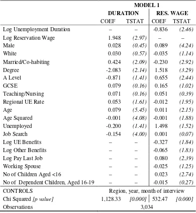
We estimate equation (2) as a system of equations by two stage least squares.7 The results are
shown in Table 2 where the first column presents the unemployment duration equation whilst
the second column presents the reservation wage equation. In accordance with the existing
literature, higher education, specifically having a degree (undergraduate or post-graduate), is
7
associated with a lower duration of unemployment. In line with the findings of Jones (1988),
the length of unemployment duration is positively related to the regional unemployment rate,
although only at the 10 percent level, as well as the age of the individual. We have also
controlled for the influence of job search upon the length of the spell of unemployment and
the results suggest that undertaking job search decreases the length of time not in work,
which is consistent with the predictions of job search theory. For example, a one standard
deviation increase in job search intensity decreases the number of days of not working by
17.5 percentage points. The elasticity of unemployment duration with respect to the
reservation wage ( ˆγ) is positive and statistically significant, supporting the predictions of job
search theory, and is similar in magnitude to that reported in existing studies, such as
Lancaster (1985) and Jones (1988), whilst being smaller in magnitude to the corresponding
elasticity found by Dolton and O’Neill (1995).
Turning to the reservation wage equation, the results suggest that individuals who are
male, highly educated and older have a higher reservation wage – findings which are broadly
consistent with previous UK evidence, see, for example, Haurin and Sridhar (2003) and
Gorter and Gorter (1993). A higher regional unemployment rate and being married or
cohabiting are associated with a lower reservation wage. Whilst the elasticity of
unemployment duration with respect to the reservation wage ( ˆλ) is elastic, the elasticity of
the reservation wage with respect to unemployment duration, in accordance with the findings
in the existing literature, is inelastic and negative at -0.84.
As discussed above, the exclusion restrictions are based upon the existing literature
and rely on identifying variables which influence unemployment duration only indirectly via
the reservation wage, such as factors which affect the costs of job search. For an instrument
to be valid, it must be correlated with the variable to be instrumented, i.e. the log reservation
wage, and uncorrelated with the log duration of unemployment. A test of including the set of
level, they are jointly significant. To be specific, benefit income is statistically significant as
is the number of dependent children under 16, which is consistent with the findings of Jones
(1988). Given that we have more than one instrument and that we are only instrumenting a
single variable, i.e. the reservation wage, it is possible to identify the model by testing the
validity of one instrument assuming the others are valid, see Cameron and Trivedi (2005). In
particular, although not reported, we find that other benefit income and the number of
children under 16 are statistically insignificant if included in the unemployment duration
equation. Thus, the over-identifying restriction that the covariates are valid instruments
appears appropriate.
To summarise, the findings accord with the existing literature in that the reservation
wage serves to increase the duration of unemployment, whilst the duration of unemployment
has a moderating influence on the reservation wage. As discussed in Section I, the expected
wage plays an important role in job search theory, although this role has not been explored
from an empirical perspective. Hence, we now focus on modeling unemployment duration,
reservation wages and expected wages, simultaneously, in order to explicitly incorporate
expected wages into the econometric framework.
IV. Reservation Wages, Expected Wages and the Duration of Unemployment
Methodology
As highlighted in the introduction, Lancaster and Chesher (1983) regard the reservation
wage, expected wage and unemployment duration as jointly determined outcomes. In
addition, they argue that job seekers might revise their reservation wage as their expected
wage (i.e. potential income) fluctuates. Hence, in a stochastic framework the introduction of
an unexpected change in labour market policy arguably acts as an exogenous shock,
impacting on the expected wage, which in turn may influence the reservation wage and,
subsequently, the duration of unemployment. In order to explore the impact of such a change
Whilst a range of labour market policies such as the national minimum wage have
been recently introduced in the UK, which have focused on increasing the returns from
employment, the WFTC, in contrast, aimed to encourage those currently in receipt of benefit
income into employment (Dilnot and McCae, 1999).8 Eligibility for WFTC depended on
hours of work (i.e. one adult in the family must work 16 hours or more a week), the number
of dependent children (under 16 or under 19 and in full-time education) and capital (less than
£8,000). Couples claimed jointly and need not be married. In addition, the scheme included
payable childcare tax credit of up to 70% of costs incurred (Brewer et al., 2006). WFTC were
introduced in October 1999 and were fully phased in by April 2000 with the principal aim of
increasing labour market participation. Indeed, Brewer et al. (2006) found that WFTC
increased the employment rate of lone mothers, reduced the labour supply of women in
couples with children, and increased the labour supply of men in couples with children.
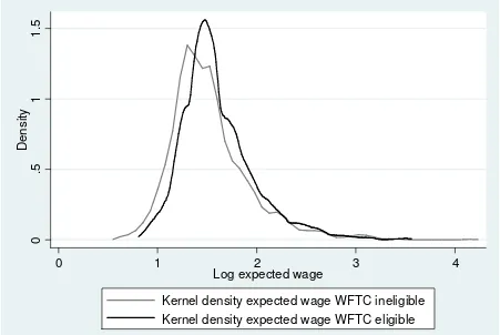
If the policy change is unexpected then a shift in the expected net income distribution
is predicted, which may affect the reservation wage and, subsequently, unemployment
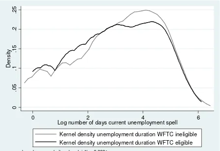
duration. Figure 4 shows the expected wage distributions by WFTC eligibility: where for
those individuals who are eligible for WFTC, the distribution is shifted to the right in
comparison to that for those individuals who are ineligible for WFTC. Figures 5 and 6 show
the reservation wage and unemployment duration distributions by WFTC eligibility,
respectively. As with the expected wage distribution, there is some evidence in the raw data
that the distribution of the reservation wage for those eligible for WFTC lies above the
distribution for those who are not eligible for WFTC. Differences in the distribution of the
duration of unemployment by WFTC eligibility are less transparent, however, in that, at
8
lower (higher) levels of unemployment duration, those eligible for WFTC have a distribution
which lies above (below) that of those individuals who are ineligible for WFTC.
With respect to the sample means, there are clear differentials by WFTC eligibility,
which are statistically significant. For example, the expected wage and reservation wage both
have a higher mean and lower variance for those eligible for WFTC, see Table 1B.
Conversely, the duration of unemployment is lower in the raw data for those who are eligible
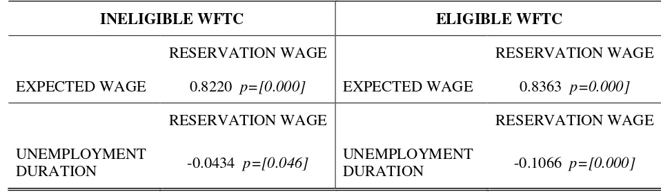
for WFTC. The raw correlations in the data between the reservation wage and unemployment
duration, and the reservation wage and the expected wage are shown in Table 1C by WFTC
eligibility. Clearly, there is a positive and statistically significant relationship between the
reservation wage and expected wage and the magnitude is larger for the sample of individuals
who are eligible for WFTC. The inverse relationship between the reservation wage and the
duration of the unemployment spell is also heightened for the sample of individuals who are
eligible for WFTC.
Given the above findings in the raw data it is interesting to explore whether the key
elasticities between the reservation wage and the duration of unemployment differ, once
wage expectations are explicitly incorporated into the model, relative to those estimated in
the two equation system specification.9 In order to explore such considerations, we model a
system of three equations by three stage least squares using Mundlak fixed effects as follows:
( )
( )
( )
( )
( )
( )
1it 1i 1
2it 2i 2
3it 3i 3
log log
log log log
log it it it it it it it it it t rw
rw t ew
ew WFTC
β γ π ε
φ λ τ θ ε
η ϕ α ε
= + + +
= + + +
= + + +
X Z
X + Z
X Z
(3)
The vector X3 contains covariates which potentially influence the expected wage of the
individual, which are based on the controls which are usually included in a Mincerian wage
9
equation, see Willis (1986), specifically: gender; ethnicity; marital status; highest level of
educational attainment; a quadratic in age; and whether the individual has had previous
employment by including their wage level from their last period of employment.
We also condition on WFTC (i.e. WFTC eligibility as described above) in the
expected wage equation, which acts as an exclusion restriction to identify the parameters of
the reservation wage equation when the expected wage is included as a covariate.10 The
exclusion restrictions used to identify the parameters of the unemployment duration equation
are as in equation (2) above. The vector Z3 contains the mean of time varying covariates to
control for fixed effects, Mundlak (1978). The parameters η and ϕ capture the influence of
variables on the expected wage and measure the elasticity of the expected wage with respect
to the introduction of WFTC.
In order to explore the robustness of our findings, we estimate a range of
specifications where WFTC is defined in four alternative ways: firstly, as a single binary
indicator denoting eligibility for WFTC in any year from 1999 onwards (i.e. ‘model 2’);
secondly, as three binary controls for eligibility between October 1999 and April 2000 (the
period when WFTC was introduced), eligibility between May 2000 and 2001 and eligibility
in 2002 (i.e. ‘model 3’); thirdly, as eligibility in 1999, i.e. eligibility status at the time of the
policy change, entered as a time invariant control from 1999 onwards (i.e. ‘model 4’); finally,
as three binary indicators each equal to unity if it is the first, second, or third year that the
individual has been eligible for WFTC (i.e. ‘model 5’). The different specifications allow us
to explore the sensitivity of the results to the definition of the exclusion condition in the
expected wage equation. For example, it may be the case that the WFTC policy reform may
by making job search more effective but not by altering individual’s expectations and their subsequent reservation wages.
10
only be a ‘surprise’ (i.e. unexpected) for the year of introduction or for the first year that the
individual is eligible.
Results
We estimate equation (3) as a system of equations by three stage least squares. The results are
shown in Tables 3 and 4 where models 2 and 3 are presented in Table 3 and models 4 and 5
are presented in Table 5.11 Across the four specifications, the first column presents the
unemployment duration equation, the second column presents the reservation wage equation,
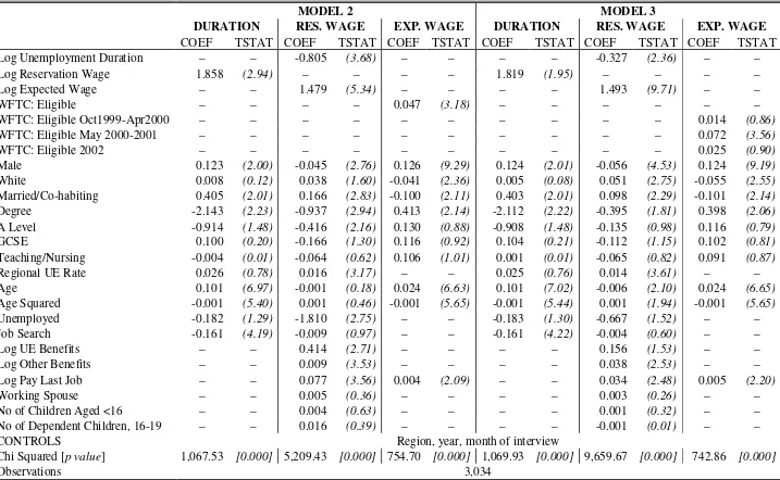
and the third column presents the expected wage equation. It is apparent that in ‘model 2’ in
Table 3, being eligible for WFTC has a positive and statistically significant influence on the
expected wage ( ˆϕ) – at approximately 5 percentage points.12 Gender, educational attainment
and age act in accordance with the direction of impact that one would expect in a wage
equation: to be specific, males and older individuals expect a higher wage as do those with
higher levels of educational attainment. In the reservation wage equation, the elasticity of the
reservation wage with respect to the expected wage is positive and elastic. Out of the
over-identifying instruments in the reservation wage equation, benefit income has a positive
impact upon the reservation wage as found by Jones (1988), Gorter and Gorter (1993) and
Dolton and O’Neill (1995). For example, a one percent increase in the level of unemployment
benefits is associated with a higher reservation wage in the order of 0.4 percentage points.
This finding is similar to the upper range found by Addison et al. (2009) for the benefit
elasticity across European countries using the non parametric approach of Lancaster and
Chesher (1983).
In terms of the key elasticities, ˆγ and ˆλ, which measure the elasticity of
unemployment duration with respect to the reservation wage and the elasticity of the
11
For brevity, we do not report the parameter estimates of π, θ and α. These results are available on request. 12
reservation wage with respect to unemployment duration, respectively, compared to the
estimates found in the two equation system, i.e. ‘model 1’, incorporating the expected wage
into the econometric framework has slightly altered the magnitude of the elasticities. To be
specific, there has been a moderate decrease in the elasticity of unemployment duration with
respect to the reservation wage from 1.95 to 1.86 and a slight increase in the elasticity of the
reservation wage with respect to unemployment duration from -0.84 to -0.81, although the
changes are not statistically significant. An increase in the reservation wage by 10 percent
reduces the chance of finding employment by around 19 percentage points. This is
comparable in magnitude to the estimate of the elasticity of unemployment duration with
respect to the reservation wage of 1.8 obtained by Lancaster (1985) in a two equation model.
In ‘model 3’ we control for WFTC eligibility by including three binary indicators,
which denote the year when the individual was eligible for WFTC: arguably if the
introduction of WFTC was an unexpected policy shock, its effect may be largest at or near
the point of introduction and potentially may dissipate thereafter. Since WFTC were not fully
implemented until April 2000, this is potentially when one might expect the influence of the
policy change to be the most pronounced. The results shown in Table 3 indeed suggest that
this is borne out by the data. To be specific, we find that eligibility for WFTC during the
induction phase, i.e. October 1999 to April 2000, has no significant statistical association
with the expected wage. The only statistically significant effect relates to eligibility between
May 2000 and 2001, which is found to increase the expected wage by 7.2 percentage points.
Finally, the specification encapsulated by ‘model 3’ serves to further moderate the magnitude
of the key elasticities ˆγ and ˆλ. Interestingly, the elasticity of the reservation wage with
respect to unemployment duration ( ˆλ) is now significantly different from that found in the
two equation model adopted in the existing literature, i.e. ‘model 1.’
In Table 4, the WFTC control is defined as where eligibility in 1999 is entered as a
time invariant binary indicator from 1999 onwards. The results suggest that the influence of
WFTC eligibility is moderated in comparison to ‘model 2’ and is only statistically significant
at the 10 percent level. This finding is perhaps not surprising given that the results of ‘model
3’ suggest that WFTC eligibility only has a statistically significant positive impact upon wage
expectations when the policy is fully implemented, i.e. May 2000. Again, the key elasiticities
in terms of magnitude, sign and elasticity remain unchanged. The final specification that is
estimated is ‘model 5’ where three binary controls are entered which represent the first,
second and third years of WFTC eligibility. Whilst the key elasticities between reservation
wages and unemployment duration are robust to this alternative definition of controlling for
WFTC eligibility, WFTC eligibility only has a statistically significant association with the
expected wage during the initial, i.e. first year, of eligibility.
To summarise, the incorporation of expected wages into the econometric framework
serves to lower the effect of the reservation wage on the duration of unemployment and
serves to moderate the inverse effect of the duration of unemployment on the reservation
wage. However, with the exception of one specification, the differentials are statistically
insignificant when compared to the two equation approach. It is interesting to note that once
the period of WFTC eligibility is explicitly taken into account, the extent to which the
elasticity of the reservation wage with respect to unemployment duration ( ˆλ) becomes
smaller in magnitude, i.e. more inelastic, is statistically significant as compared to the two
equation model.13
13
V. Conclusion
In this paper, we have extended the structural model of Jones (1988) to incorporate the role of
expected wages. Although the expected wage plays an important role in theoretical models of
job search and labour market participation, to the authors’ knowledge, this is the first paper to
explicitly incorporate the expected wage into an empirical framework, which jointly models
the length of unemployment duration (in the context of incomplete spells), the reservation
wage and the expected wage. As such, we make an important contribution to the existing
empirical literature in this area. In our econometric framework, an exogenous policy shock,
i.e. the introduction of WFTC, is allowed to influence the expected net income distribution,
which in turn influences the reservation wage and hence the duration of not being in work.
Our empirical results suggest that the introduction of WFTC had a positive influence
on expected wages, which in turn were positively associated with reservation wages. In
addition, we find that the magnitude of the elasticity of unemployment duration with respect
to the reservation wage and the elasticity of the reservation wage with respect to
unemployment duration are both reduced in absolute terms relative to the corresponding
elasticities estimated in the two equation model, which does not explicitly incorporate wage
expectations. However, with the exception of one specification, the differentials in the key
elasticities across the two equation and three equation models are not statistically significant.
The effect of incorporating wage expectations only has a significant effect upon the
differentials in the key elasticities when we explicitly take into account the period of WFTC
eligibility. To be specific, the results suggest that the sensitivity of reservation wages with
respect to unemployment duration becomes considerably less elastic, changing from -0.84
(‘model 1’) to -0.33 (‘model 3’). Such a finding is consistent with individuals becoming more
informed about labour market conditions once wage expectations and the ‘surprise’ element
Our empirical findings highlight the importance of incorporating wage expectations in
the analysis of the behaviour and decision-making of those individuals who are not in work,
as well as contributing more generally to the sparse, yet growing, empirical literature
exploring the role and implications of expectations at the individual and household level.
Moreover, given the influence of wage expectations on reservation wages, it is apparent that
policy-makers may be able to influence the reservation wages of those out of work by
focusing on the determinants of expected wages. For example, the role of Government
agencies such as Job Centre Plus in the UK, which support people of working age from
welfare into work and aid employers in filling vacancies, in disseminating advice and
information to those out of work, may serve to not only help make job search more effective,
with the aim of increasing the arrival rate of job offers, but also to help to shape the wage
expectations of the unemployed. It is apparent that understanding the eligibility and operation
of tax credit systems can be daunting for those out of work. Given that such aspects of the tax
system are primarily designed to encourage those on benefits into the labour market via
altering take-home wages, an important, if not essential, part of the process is to help to
inform those out of work about the operation of tax credits in order to influence their wage
expectations and thereby to encourage labour market participation.
References
Addison, J., Centeno, M. and P. Portugal (2009) Unemployment Benefits and Reservation:
Key Elasticities from a Stripped-Down Job Search Approach. Economica
(forthcoming).
Barth, E. (1997) Firm-Specific Seniority and Wages. Journal of Labor Economics, 15(3), 495-506.
Blackaby, D. H., Latreille, P., Murphy, P. D., O’Leary, N. C. and P. J. Sloane (2007) An
Analysis of Reservation Wages for the Economically Inactive. Economics Letters, 97(1), 1-5.
Brewer, M., Duncan, A., Shephard, A. and M. Suárez (2006) Did Working Families Tax
Credit Work? The Impact of In-Work Support on Labour Supply in Great Britain.
Brown, S., Garino, G., Taylor, K. and S. Wheatley Price (2005) Debt and Financial
Expectations: An Individual and Household Level Analysis. Economic Inquiry,43, 100-20.
Brown, S., G. Garino and K. B. Taylor (2008) Mortgages and Financial Expectations: A
Household Level Analysis. Southern Economic Journal, 74(3), 857-78.
Cameron, A. and P. Trivedi (2005) Microeconometrics: Methods and Applications.
Cambridge University Press.
Das, M. and A. van Soest (1999) A Panel Data model for Subjective Information on
Household Income Growth. Journal of Economic Behaviour and Organisation, 40, 409-26.
Dilnot, A. and McCae, J. (1999) Family Credit and the Working Family Tax Credit. IFS
Briefing Note Number 3.
Dolton, P. and D. O’Neill (1995) The Impact of Restart on Reservation Wages and
Long-Term Unemployment. Oxford Bulletin of Economics and Statistics, 57(4), 451-70. Gorter, D. and C. Gorter (1993) The Relationship Between Unemployment Benefits, the
Reservation Wage and Search Duration. Oxford Bulletin of Economics and Statistics. 55, 199-214.
Haurin, D. R. and K. S. Sridhar (2003) The Impact of Local Unemployment Rates on
Reservation Wages and the Duration of Search for a Job. Applied Economics, 35, 1469-76.
Hofler, R. A. and K. J. Murphy (1994) Estimating Reservation Wages of Employed Workers
Using a Stochastic Frontier. Southern Economic Journal, 60, 961-76.
Hui, WT. (1991) Reservation Wage Analysis of Unemployed Youths in Australia. Applied Economics, 23, 1341-50.
Jones, S. (1988) The Relationship Between Unemployment Spells and Reservation Wages as
a Test of Search Theory. Quarterly Journal of Economics, 103(4), 741-65.
Kiefer, N. M. and G. R. Neumann (1979) An Empirical Job-Search Model with a Test of the
Constant Reservation Wage Hypothesis. Journal of Political Economy, 87, 89-107. Kirby, S. and R. Riley (2008) The external Returns to Education: UK Evidence Using
Repeated Cross-Sections. Labour Economics, 15(4), 619-30.
Korkeamäki, O. and T. Kyyrä (1996) A Gender Wage Gap Decomposition for Matched
Employer-Employee Data. Labour Economics, 13(5), 611-38.
Lancaster, T. and A. Chesher (1983) An Econometric Analysis of Reservation Wages.
Econometrica, 51, 1661-76.
Lancaster, T. and A. Chesher (1984) Simultaneous Equations with Endogenous Hazards. In
Studies in Labor Market Dynamics, Neumann, G. R. and Westergaard-Nielsen, N. C.
(eds.), Springer-Verlag, Heidelberg.
Manning, A. (2005) You Can’t Always Get What You Want: the Impact of the UK Job
Seeker’s Allowance. Centre for Economic Performance, LSE, Discussion Paper
Number 697.
Manski, C. (2004) Measuring Expectations. Econometrica, 72, 1329–76.
McKay, S. (2003) Working Families' Tax Credit in 2001, Department of Work & Pensions
Research Report Number 181.
Mortensen, D. T. (1986) Job Search and Labor Market Analysis, in O. Ashenfelter and R.
Layard (eds.) Handbook of Labor Economics, Volume 2, North-Holland.
Mortensen, D. T. and C. A. Pissarides (1999) New Developments in Models of Search in the
Labor Market, in O. Ashenfelter and D. Card (eds.) Handbook of Labor Economics, Volume 3, North Holland.
Mundlak, Y. (1978) ‘On the Pooling of Time Series and Cross Section Data’, Econometrica, 46, 69-85.
Pissarides, C. A. (2000) Equilibrium Unemployment Theory, Second Edition. MIT Press,
Cambridge, MA.
Souleles, N. S. (2004) Expectations, Heterogenous Forecast Errors, and Consumption: Micro
Evidence from the Michigan Consumer Sentiment Surveys. Journal of Money, Credit, and Banking, 36, 39-72.
Schweitzer, M. (2003) Ready, Willing and Able? Measuring Labour Market Availability in
the UK. Bank of England Working Paper Number 186.
Willis, R. (1986) Wage Determinants: A Survey and Reinterpretation of Human Capital
Figure 1: The Distribution of the Log Reservation Wage, 1996 to 2002
0
5
1
0
1
5
2
0
P
e
rc
e
n
t
0 1 2 3 4
Figure 2: The Distribution of the Log Expected Wage, 1996 to 2002
0
5
1
0
1
5
2
0
P
e
rc
e
n
t
1 2 3 4
Figure 3: The Distribution of the Log Number of Days Currently Not in Work, 1996 to 2002
0
2
4
6
8
P
e
rc
e
n
t
0 2 4 6
Figure 4: Density Plot of the Log Expected Wage by WFTC Eligibility
0
.5
1
1
.5
D
e
n
s
it
y
0 1 2 3 4
Log expected wage
Kernel density expected wage WFTC ineligible Kernel density expected wage WFTC eligible
Figure 5: Density Plot of the Log Reservation Wage by WFTC Eligibility
0
.5
1
1
.5
2
D
e
n
s
ity
1 2 3 4
Log reservation wage
Kernel density reservation wage WFTC ineligible Kernel density reservation wage WFTC eligible
Figure 6: Density Plot of the Log Duration of Unemployment by WFTC Eligibility
0
.0
5
.1
.1
5
.2
.2
5
D
e
n
s
it
y
0 2 4 6
Log number of days current unemployment spell
Kernel density unemployment duration WFTC ineligible Kernel density unemployment duration WFTC eligible
Table 1A: Summary Statistics
MEAN STD. DEV MIN MAX
Log Unemployment Duration 3.041 1.555 0 6.136
Log Reservation Wage 1.438 0.356 0.613 3.992
Log Expected Wage 1.549 0.389 0.693 4.169
Male 0.406 0.491 0 1
White 0.818 0.386 0 1
Married/Co-habiting 0.680 0.467 0 1
Degree 0.069 0.253 0 1
A Level 0.116 0.321 0 1
GCSE 0.220 0.414 0 1
Teaching/Nursing Qualification 0.187 0.390 0 1
Regional Unemployment (UE) Rate 5.976 1.590 3.3 11.1
Age 37.531 11.609 16 65
Unemployed 0.380 0.486 0 1
Job Search Index 0.835 1.139 0 3
Log UE Benefits 1.377 1.012 0 3.765
Log Other Benefits 4.045 1.992 0 7.233
Log Pay Last Job 2.013 3.036 0 9.392
Working Spouse 0.383 0.486 0 1
No of Children Aged <16 1.074 1.172 0 7
No of Dependent Children, Aged 16-19 0.061 0.257 0 3
WFTC: Eligible 0.302 0.459 0 1
WFTC: Eligible Oct 1999 – Apr 2000 0.193 0.395 0 1
WFTC: Eligible May 2000 – 2001 0.115 0.319 0 1
WFTC: Eligible 2002 0.093 0.291 0 1
WFTC: 1999 Eligibility 0.157 0.364 0 1
WFTC: 1st year Eligible 0.265 0.442 0 1
WFTC: 2nd year Eligible 0.047 0.212 0 1
WFTC: 3rd year Eligible 0.012 0.108 0 1
Table 1B: Mean and Standard Deviation of Log Unemployment Duration, Log Reservation Wage and Log Expected Wage by WFTC Eligibility
INELIGIBLE WFTC ELIGIBLE WFTC
MEAN STD. DEV MEAN STD. DEV
Log Unemployment Duration 3.090 1.543 2.926 1.579
Log Reservation Wage 1.419 0.368 1.482 0.323
Log Expected Wage 1.525 0.395 1.605 0.368
Observations 2,118 916
Table 1C: Correlations between Log Unemployment Duration and Log Reservation Wage and between Log Reservation Wage and Log Expected Wage by WFTC Eligibility
INELIGIBLE WFTC ELIGIBLE WFTC
RESERVATION WAGE RESERVATION WAGE
EXPECTED WAGE 0.8220 p=[0.000] EXPECTED WAGE 0.8363 p=0.000]
RESERVATION WAGE RESERVATION WAGE
UNEMPLOYMENT
DURATION -0.0434 p=[0.046]
UNEMPLOYMENT
[image:30.612.74.553.313.454.2]Table 2: 2SLS Model of Unemployment Duration and the Reservation Wage
MODEL 1
DURATION RES. WAGE
COEF TSTAT COEF TSTAT
Log Unemployment Duration – – -0.836 (2.46)
Log Reservation Wage 1.948 (2.97) – –
Male 0.028 (0.45) 0.089 (4.24)
White 0.030 (0.57) -0.035 (1.14)
Married/Co-habiting 0.424 (2.09) -0.230 (2.92)
Degree -2.083 (2.14) 1.518 (3.29)
A Level -0.871 (1.41) 0.655 (2.44)
GCSE 0.079 (0.16) 0.165 (1.02)
Teaching/Nursing 0.071 (0.16) 0.051 (0.39)
Regional UE Rate 0.053 (1.61) -0.012 (1.95)
Age 0.079 (5.45) 0.011 (2.15)
Age Squared -0.001 (4.08) -0.001 (1.88)
Unemployed -0.200 (1.41) 1.498 (1.52)
Job Search -0.154 (4.00) 0.001 (0.07)
Log UE Benefits – – -0.327 (1.84)
Log Other Benefits – – -0.065 (1.83)
Log Pay Last Job – – 0.080 (2.39)
Working Spouse – – -0.025 (1.25)
No of Children Aged <16 – – 0.023 (2.74)
No of Dependent Children, Aged 16-19 – – -0.015 (0.27)
CONTROLS Region, year, month of interview
Chi Squared [p value] 1,128.33 [0.000] 532.47 [0.000]
Table 3: 3SLS Model of Unemployment Duration, Reservation Wages and Expected Wages
MODEL 2 MODEL 3
DURATION RES. WAGE EXP. WAGE DURATION RES. WAGE EXP. WAGE
COEF TSTAT COEF TSTAT COEF TSTAT COEF TSTAT COEF TSTAT COEF TSTAT
Log Unemployment Duration – – -0.805 (3.68) – – – – -0.327 (2.36) – –
Log Reservation Wage 1.858 (2.94) – – – – 1.819 (1.95) – – – –
Log Expected Wage – – 1.479 (5.34) – – – – 1.493 (9.71) – –
WFTC: Eligible – – – – 0.047 (3.18) – – – – – –
WFTC: Eligible Oct1999-Apr2000 – – – – – – – – – – 0.014 (0.86)
WFTC: Eligible May 2000-2001 – – – – – – – – – – 0.072 (3.56)
WFTC: Eligible 2002 – – – – – – – – – – 0.025 (0.90)
Male 0.123 (2.00) -0.045 (2.76) 0.126 (9.29) 0.124 (2.01) -0.056 (4.53) 0.124 (9.19)
White 0.008 (0.12) 0.038 (1.60) -0.041 (2.36) 0.005 (0.08) 0.051 (2.75) -0.055 (2.55)
Married/Co-habiting 0.405 (2.01) 0.166 (2.83) -0.100 (2.11) 0.403 (2.01) 0.098 (2.29) -0.101 (2.14)
Degree -2.143 (2.23) -0.937 (2.94) 0.413 (2.14) -2.112 (2.22) -0.395 (1.81) 0.398 (2.06)
A Level -0.914 (1.48) -0.416 (2.16) 0.130 (0.88) -0.908 (1.48) -0.135 (0.98) 0.116 (0.79)
GCSE 0.100 (0.20) -0.166 (1.30) 0.116 (0.92) 0.104 (0.21) -0.112 (1.15) 0.102 (0.81)
Teaching/Nursing -0.004 (0.01) -0.064 (0.62) 0.106 (1.01) 0.001 (0.01) -0.065 (0.82) 0.091 (0.87)
Regional UE Rate 0.026 (0.78) 0.016 (3.17) – – 0.025 (0.76) 0.014 (3.61) – –
Age 0.101 (6.97) -0.001 (0.18) 0.024 (6.63) 0.101 (7.02) -0.006 (2.10) 0.024 (6.65)
Age Squared -0.001 (5.40) 0.001 (0.46) -0.001 (5.65) -0.001 (5.44) 0.001 (1.94) -0.001 (5.65)
Unemployed -0.182 (1.29) -1.810 (2.75) – – -0.183 (1.30) -0.667 (1.52) – –
Job Search -0.161 (4.19) -0.009 (0.97) – – -0.161 (4.22) -0.004 (0.60) – –
Log UE Benefits – – 0.414 (2.71) – – – – 0.156 (1.53) – –
Log Other Benefits – – 0.009 (3.53) – – – – 0.038 (2.53) – –
Log Pay Last Job – – 0.077 (3.56) 0.004 (2.09) – – 0.034 (2.48) 0.005 (2.20)
Working Spouse – – 0.005 (0.36) – – – – 0.003 (0.26) – –
No of Children Aged <16 – – 0.004 (0.63) – – – – 0.001 (0.32) – –
No of Dependent Children, 16-19 – – 0.016 (0.39) – – – – -0.001 (0.01) – –
CONTROLS Region, year, month of interview
Chi Squared [p value] 1,067.53 [0.000] 5,209.43 [0.000] 754.70 [0.000] 1,069.93 [0.000] 9,659.67 [0.000] 742.86 [0.000]
Table 4: 3SLS Model of Unemployment Duration, Reservation Wages and Expected Wages
MODEL 4 MODEL 5
DURATION RES. WAGE EXP. WAGE DURATION RES. WAGE EXP. WAGE
COEF TSTAT COEF TSTAT COEF TSTAT COEF TSTAT COEF TSTAT COEF TSTAT
Log Unemployment Duration – – -0.611 (3.43) – – – – -0.517 (3.52) – –
Log Reservation Wage 1.891 (1.97) – – – – 1.841 (1.93) – – – –
Log Expected Wage – – 1.486 (7.27) – – – – 1.488 (8.62) – –
WFTC: 1999 Eligibility – – – – 0.014 (1.78) – – – – – –
WFTC: 1st year Eligible – – – – – – – – – – 0.046 (3.11)
WFTC: 2nd year Eligible – – – – – – – – – – 0.051 (1.71)
WFTC: 3rd year Eligible – – – – – – – – – – 0.017 (0.31)
Male 0.124 (2.00) -0.051 (3.46) 0.129 (9.52) 0.124 (2.00) -0.052 (3.91) 0.126 (9.30)
White 0.008 (0.12) 0.047 (2.20) -0.057 (3.43) 0.007 (0.11) 0.044 (2.23) -0.043 (2.41)
Married/Co-habiting 0.408 (2.02) 0.139 (2.68) -0.098 (2.08) 0.404 (2.00) 0.124 (2.93) -0.099 (2.10)
Degree -2.165 (2.25) -0.730 (2.69) 0.446 (2.31) -2.131 (2.21) -0.615 (2.64) 0.413 (2.14)
A Level -0.924 (1.50) -0.308 (1.83) 0.140 (0.95) -0.912 (1.48) -0.249 (1.69) 0.127 (0.86)
GCSE 0.099 (0.20) -0.148 (1.28) 0.124 (0.98) 0.102 (0.20) -0.137 (1.31) 0.116 (0.92)
Teaching/Nursing -0.011 (0.02) -0.072 (0.77) 0.130 (1.25) -0.003 (0.01) -0.068 (0.80) 0.106 (1.02)
Regional UE Rate 0.025 (0.76) 0.015 (3.31) – – 0.025 (0.75) 0.015 (3.58) – –
Age 0.101 (6.98) -0.003 (0.80) 0.025 (6.73) 0.101 (6.98) -0.003 (1.39) 0.024 (6.62)
Age Squared -0.001 (5.40) 0.001 (0.95) -0.001 (5.75) -0.001 (5.40) 0.001 (1.41) -0.001 (5.65)
Unemployed -0.181 (1.28) -1.335 (2.40) – – -0.183 (1.30) -1.126 (2.38) – –
Job Search -0.160 (4.18) -0.007 (0.90) – – -0.161 (4.19) -0.005 (0.72) – –
Log UE Benefits – – 0.307 (2.37) – – – – 0.260 (2.36) – –
Log Other Benefits – – 0.064 (3.33) – – – – 0.056 (3.48) – –
Log Pay Last Job – – 0.059 (3.36) 0.005 (2.30) – – 0.051 (3.52) 0.005 (2.12)
Working Spouse – – 0.004 (0.29) – – – – 0.004 (0.32) – –
No of Children Aged <16 – – 0.003 (0.52) – – – – 0.002 (0.50) – –
No Dependent Children, 16-19 – – 0.009 (0.26) – – – – 0.006 (0.19) – –
CONTROLS Region, year, month of interview
Chi Squared [p value] 1,065.84 [0.000] 6,413.58 [0.000] 736.52 [0.000] 1,064.35 [0.000] 7,970.17 [0.000] 744.87 [0.000]