Transient climate response estimated from radiative forcing and observed temperature change

This is a repository copy of

Transient climate response estimated from radiative forcing

and observed temperature change

.

White Rose Research Online URL for this paper:

http://eprints.whiterose.ac.uk/43312/

Article:

Gregory, JM and Forster, PM (2008) Transient climate response estimated from radiative

forcing and observed temperature change. Journal of Geophysical

Research-Atmospheres, 113 (D23). ISSN 0148-0227

https://doi.org/10.1029/2008JD010405

eprints@whiterose.ac.uk https://eprints.whiterose.ac.uk/

Reuse

See Attached

Takedown

If you consider content in White Rose Research Online to be in breach of UK law, please notify us by

Transient climate response estimated from radiative forcing

and observed temperature change

J. M. Gregory1,2 and P. M. Forster3

Received 13 May 2008; revised 19 September 2008; accepted 7 October 2008; published 10 December 2008.

[1] Observations and simulations (using the HadCM3 AOGCM) of time-dependent

twentieth-century climate change indicate a linear relationshipF=rDTbetween radiative

forcing Fand global mean surface air temperature change _DT. The same is a good description of_DTfrom CMIP3 AOGCMs integrated with CO2increasing at 1% per year

compounded. The constant ‘‘climate resistance’’r is related to the transient climate

response (TCR,_DTat the time of doubled CO2under the 1% CO2scenario). Disregarding

any trend caused by natural forcing (volcanic and solar), which is small compared with the trend in anthropogenic forcing, we estimate that the real-world TCR is 1.3 –2.3 K (5–95% uncertainty range) from the data of 1970– 2006, allowing for the effect of unforced variability on longer timescales. The climate response to episodic volcanic forcing cannot be described by the same relationship and merits further investigation; this constitutes a systematic uncertainty of the method. The method is quite insensitive to the anthropogenic aerosol forcing, which probably did not vary much during 1970 –2006 and therefore did not affect the trend in _DT. Our range is very similar to the range of recent AOGCM results for the TCR. Consequently projections for warming during the twenty-first century under the SRES A1B emissions scenario made using the simple empirical relationshipF=rDTagree with the range of AOGCM results for that scenario.

Our TCR range is also similar to those from observationally constrained model-based methods.

Citation: Gregory, J. M., and P. M. Forster (2008), Transient climate response estimated from radiative forcing and observed temperature change,J. Geophys. Res.,113, D23105, doi:10.1029/2008JD010405.

1. Introduction

[2] Climate models show that continued emissions of

greenhouse gases at or above current rates would cause climate change during the twenty-first century that would very likely be larger than that observed in the twentieth century, but there are great uncertainties about the size of the projected changes [Meehl et al., 2007]. The magnitude of global climate change on multiannual timescales is conventionally measured by the global mean surface air temperature change DT. This quantity is useful because general circulation models (GCMs) suggest that many aspects of projected climate change scale withDTi.e., the changeDV(x,t) in some quantityVsuch as temperature or precipitation, as a function of geographical location xand timet, can be approximated as the productDV=P(x)DT(t) of a constant spatial patternPwith a magnitude represented byDT[Mitchell et al., 1999;Huntingford and Cox, 2000]. [3] The magnitude of the influence of a forcing agent is

measured by its radiative forcingF, which is usually defined

as the change in global mean net downward radiation at the tropopause caused by adding the forcing agent, either instantaneously, or with allowance for stratospheric adjust-ment. Recent work [Shine et al., 2003;Gregory et al., 2004; Hansen et al., 2005;Gregory and Webb, 2008;Williams et al., 2008; Andrews and Forster, 2008] suggests a more general definition ofFas the net global mean heat flux into the climate system caused by the forcing agent without any climate response having occurred. In response to F, the magnitude of climate change is determined by a heat balance

N_¼FaDT; ð1Þ

whereNis the net heat flux into the climate system (W m2) andais the climate sensitivity parameter (W m2K1) [e.g., Gregory et al., 2004]. The term aDT is the radiative

response of the climate system to forcing on multiannual timescales. For a stable systema> 0, so that if a positive

forcing is imposed, such as by an increase in greenhouse gas concentrations, the net response is to lose more heat to space, and thus to tend to regain a steady state.

[4] When the system has reached a new steady state, in

whichN= 0 by definition, the magnitude of climate change depends on forcing and feedback according toDT=F/a. In

the particular case of a doubling of the CO2concentration,

for which F= F2,DT is usually called the ‘‘equilibrium 1_{Department of Meteorology, Walker Institute for Climate System}

Research, University of Reading, Reading, UK. 2_{Met Office Hadley Centre, Exeter, UK.} 3

School of Earth and Environment, University of Leeds, Leeds, UK.

Copyright 2008 by the American Geophysical Union. 0148-0227/08/2008JD010405

climate sensitivity’’ DT2, with DT2 = F2/a. The real

climate is however never in a steady state, and during time-dependent change the rate of storage of heat also has an influence according to DT = (F N)/a. On multiannual

timescales, the storage of heat is overwhelmingly in the ocean [Levitus et al., 2001; Bindoff et al., 2007]. The heat balance indicates that during time-dependent climate change a greater rate of ocean heat uptake means a smallerDTfor a given forcing.

[5] The important influence of heat storage on

time-dependent change limits the practical usefulness of the equilibrium climate sensitivity in comparing simulations of climate change for the coming century. ThereforeCubasch et al.[2001] introduced a new metric, the ‘‘transient climate response’’ (TCR), defined as DT for the time of doubled CO2in a scenario in which CO2 increases at 1% per year

compounded. This is a commonly used idealized scenario for studies of climate change with atmosphere-ocean general circulation models (AOGCMs). At 1% per year, the time for doubling is 70 years, and in practice a time-mean over years 61 – 80 is used to evaluate the TCR (=(F2N)/a).

The TCR is less than DT2 (=F2/a) because the ocean

heat uptakeN> 0.

[6] One way to describe the ocean’s role is as thermal

inertia, with N = CdDT/dt, where C is a constant heat capacity [Frame et al., 2005]. For forced climate change on multidecadal timescales, the effective heat capacity C is greater than that of the ocean ‘‘mixed layer,’’ and is actually not constant [Keen and Murphy, 1997; Watterson, 2000], because the ocean is not well-mixed, and the vertical profile of temperature change is time-dependent. An alternative description isN=kDT, wherekis the ‘‘ocean heat uptake

efficiency’’ [Gregory and Mitchell, 1997; Raper et al., 2002]. This formulation views the deep ocean as a heatsink, into which the surface climate loses heat in a way analogous to its heat loss to space. It permits the influences of climate feedback and ocean heat uptake to be compared, since a

and k have the same units. Like climate sensitivity, this

formulation of ocean heat uptake is a model-based result. It is evident that its validity is restricted; it cannot be correct for steady state climate change, because N _! 0 as DT approaches its equilibrium value, so the efficiency of ocean heat uptake must decline. The formulation was proposed only as a description for a system in a time-dependent state forced by a scenario with a fairly steadily increasing forcing.

[7] WhenN=kDTholds, we can write the heat balance

of the climate system asF=rDTwithrk+a, which we

call the ‘‘climate resistance,’’ because it is the reciprocal of the climate response. Unlike the formulation with a thermal inertia, the relationship F = rDT has no timescale. It

suggests that climate change tracks radiative forcing. The aim of this paper is to examine the applicability of this relationship to projected and recent past climate change.

2. Results From 1% CO2 Experiments 2.1. Climate Resistance and TCR

[8] Many AOGCMs in the Coupled Model

Intercompar-ison Project phase 3 (CMIP3) of the World Climate Research Programme (WCRP) have been run under the 1% CO2scenario. Give forcing due to CO2alone, we

can evaluate climate resistancerfrom the runs in this data

set. To obtain r, we use ordinary least squares linear

regression (OLS) ofF against DT for years 1 – 70, during which CO2is increasing. In a set of 16 CMIP3 AOGCMs,

the correlation coefficients for decadal-meanFwith decadal-meanDTexceed 0.98 in almost every case, indicating that linearity is a very good assumption. Because of the high correlation, the results from OLS regression are practically identical regardless of whether DT or F is taken as the independent variable.

[9] We adopt a standard value ofF2= 3.7 W m2for the

forcing due to doubled CO2[Myhre et al., 1998], which is

close to the average of AOGCM values reported byForster and Taylor [2006]. AOGCMs actually have a spread of O(10)% in the 2 CO2 forcing [Collins et al., 2006;

Forster and Taylor, 2006]. Furthermore,Gregory and Webb [2008], Williams et al. [2008] and Andrews and Forster [2008] show that the spread may be greater still if rapid tropospheric adjustment processes are counted in the forc-ing, in an analogous way to stratospheric adjustment. For comparability with previous results, which likewise use a standard value for F2, we ignore these issues here. Con-sequently the uncertainty inrmay be underestimated (see

also section 6).

[10] The regressions of decadal-meanFagainstDTin our

set of AOGCMs give a 5 – 95% confidence interval forrof

2.0 ± 0.7 W m2 K1, treating it as having a normal distribution (Table 1 and Figure 1). Since F = rDT, the

TCR can then be simply evaluated as F2/r, the DT that

corresponds toF2. The modelrrange gives a TCR range

of 1.4 – 2.6 K (median 1.8 K; the uncertainty is skewed because TCR/1/r). The model TCR range evaluated by

this method is not sensitive to the choice of F2, because

F2is used first to computeFand then to convertrto TCR,

and these appearances ofF2cancel each other.

[11] The TCR range calculated fromris of course similar

to the actual range ofDTat the time of 2 CO2i.e., the

definition of TCR. From the TCR values given byRandall et al.[2007] for our set of models, we consequently obtain almost the same range ofr(Table 1).

2.2. Climate Feedback and Ocean Heat Uptake [12] Raper et al.[2002] calculatedaandkfor an earlier

set of AOGCMs using the means of F, N and DT over years 61 – 80 of 1% CO2experiments, i.e., asa= (FN)/

DTandk=N/DT.Dufresne and Bony[2008] have recently

done the same for the CMIP3 AOGCMs. Here we evaluate them by OLS regression of decadal-mean FN and N respectively against DT, as for r. The results fora andk

are shown in Table 1 and Figure 1. The 5 – 95% ranges are 1.4 ± 0.6 and 0.6 ± 0.2 W m2 K1respectively, treating them as normal distributions. There is a tendency for oura

to be larger andksmaller than in the results ofDufresne and Bony[2008]. This is caused by the ‘‘cold start’’ effect in the 1% runs [Hasselmann et al., 1993; Keen and Murphy, 1997], which means the regression of Nagainst DT tends to have a small positive intercept, and a smaller slope than a line drawn from the origin to the point of 2CO2i.e., the

ratioN/DTused byDufresne and Bony[2008]. The differ-ence thus reflects the fact thatN/DTis not exact.

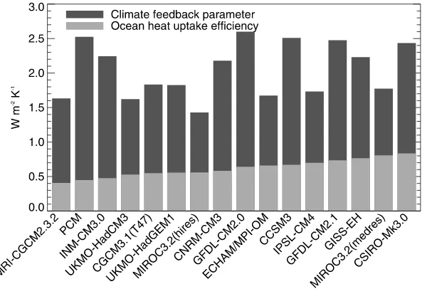
[13] These figures show that on average climate feedback

is about twice the size of ocean heat uptake, but the relative

importance ofaandkvaries among models. In some (e.g.,

PCM) ocean heat uptake is much smaller than climate feedback, while in others (e.g., MIROC3.2, both resolu-tions) they are comparable. Ifaandkare both constant, the

realized warming DT at any time in a given model is a constant fraction of the equilibrium warmingDTeqmfor the

forcing, since F = aDTeqm ) DT/DTeqm = a/(a + k).

Models with a larger khave a smaller realized fraction of

warming at any time.

[14] Raper et al. [2002] found that in the set of models

they considered there was an anticorrelation betweenaand k; large equilibrium climate sensitivity (smalla) tended to

go with large ocean heat uptake efficiency (large k). This

tendency meant that the range of TCR was smaller than if

the two factors had been independent, and they tentatively suggested physical mechanisms which might be responsi-ble. In the CMIP3 models, however, this tendency is absent, as noted also by Plattner et al. [2008]. The correlation coefficient betweena and kacross the CMIP3 models is

0.1, not significantly different from zero.

3. Climate Resistance From Simulated Past Changes

[15] The previous section shows that constantris a good

approximation in the idealized 1% CO2scenario up to 2

CO2, but that there is a large model uncertainty in r. We

wish to consider whether r can be evaluated from past

Figure 1. Climate feedback parameteraand ocean heat uptake efficiencykin a set of 16 AOGCMs,

from Table 1. The total height of each bar is the climate resistancer=a+k. The models are arranged in

order of incre .

Table 1. Climate Feedback Parametera, Ocean Heat Uptake Efficiencyk, and Climate Resistancer(All in W m2K1) Calculated by OLS Regression of Decadal-MeanFN,N, andFRespectively AgainstDTUnder a Scenario of CO2Increasing at 1% per Year for

70 Years in a Set of AOGCMsa

Model

Regression AR4 D&B

DT2/DT1

a k r r a k

CCSM3 1.84 0.67 2.51 2.5 – – 1.3

CGCM3.1(T47) 1.28 0.55 1.83 1.9 – – 1.3

CNRM-CM3 1.60 0.58 2.18 2.3 1.2 0.8 1.3

CSIRO-Mk3.0 1.60 0.83 2.44 2.6 – – –

ECHAM/MPI-OM 1.01 0.66 1.67 1.7 0.9 0.6 1.5

GFDL-CM2.0 1.96 0.64 2.60 2.3 1.2 0.5 1.5

GFDL-CM2.1 1.74 0.73 2.48 2.5 1.4 0.8 1.4

GISS-EH 1.46 0.77 2.23 2.3 – – –

INM-CM3.0 1.77 0.48 2.24 2.3 1.5 0.6 1.5

IPSL-CM4 1.03 0.70 1.73 1.8 1.0 0.8 1.3

MIROC3.2(hires) 0.87 0.56 1.43 1.4 – – –

MIROC3.2(medres) 0.97 0.81 1.77 1.8 0.9 0.8 1.4

MRI-CGCM2.3.2 1.23 0.41 1.63 1.7 1.5 0.6 1.1

PCM 2.08 0.45 2.52 2.8 1.5 0.6 1.1

UKMO-HadCM3 1.09 0.53 1.62 1.9 1.0 0.6 –

UKMO-HadGEM1 1.27 0.56 1.87 1.9 – – 1.3

Ensemble 1.4 ± 0.6 0.6 ± 0.2 2.0 ± 0.7 2.1 ± 0.7

a

The uncertainties in the ‘‘Ensemble’’ row are the 5 – 95% range assuming a normal distribution for the models. The results are compared withr

climate change. In this section we evaluate the climate resistance from simulations of the last 150 years carried out with the HadCM3 AOGCM [Gordon et al., 2000], in order to test whetherrthus obtained is consistent with the

results of the HadCM3 1% CO2experiment.

[16] Both temperature change DT and radiative forcing

F are defined relative to a steady state climate in which the forcing agents are constant. In AOGCM simulations of recent climate change, this unperturbed climate is often taken to be the late nineteenth century. However, if we suppose that the perturbations are small enough to be treated as linear (an assumption that is implicit in the use of a constantr) we do not need to know the steady state in order

to evaluater, which depends only on the slope ofFagainst

DTand is unaffected by constant offsets [cf.Gregory et al., 2002;Forster and Gregory, 2006].

3.1. Radiative Forcing

[17] The main radiative forcing agents of recent climate

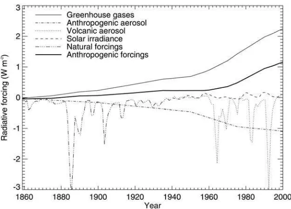
change are the following. Greenhouse gases (carbon dioxide, methane, nitrous oxide, halocarbons and ozone) make the largest contribution. Anthropogenic aerosol (the albedo and cloud effects of sulfate aerosol and black carbon) has a net negative forcing, offsetting a substantial part of the positive greenhouse-gas forcing. Volcanic aerosol has an episodically large negative forcing, following explosive eruptions, such as those of Krakatau (1883), Agung (1963), El Chichon (1982) and Pinatubo (1991); after each, it decays over a few years as the aerosol settles out of the stratosphere. Solar irradiance varies with the 11-year cycle, but has rather small longer term trends.

[18] Time series of these radiative forcings as used in

HadCM3 simulations of the past are shown in Figure 2. (HadCM3 does not simulate the forcing due to black carbon aerosol.) These forcings are consistent within uncertainties with the current best estimates for the real world (section 4). When all forcings are included in the model, the simulated

DT follows observations remarkably well [Stott et al., 2000]. The relative influences of these forcings upon twentieth-century climate change has been studied in great detail by many workers on detection and attribution of climate change [e.g.,IDAG, 2005] using AOGCM experi-ments like those with HadCM3, leading to the conclusion that ‘‘greenhouse gas forcing has very likely caused most of the observed global warming over the last 50 years’’ [Hegerl et al., 2007].

3.2. Simulations With Anthropogenic Forcing Only [19] We first consider the results from an ensemble of

four experiments with anthropogenic forcing onlyFGAi.e., greenhouse-gas and aerosol [Stott et al., 2000]. (In the next subsection we consider natural forcing as well i.e., volcanic and solar.) We obtain rby regressing DTGA againstFGA.

This assumes there is no uncertainty in the values ofF; the best fit slope is the one which minimizes the RMS deviation inDTof the data points from the regression line. This is appropriate because the forcing in the model is precisely known and effectively prescribed as a function of time. On the other hand, there is scatter in DT, due to unforced internal variability of the climate system, for example variability in cloudiness leading to fluctuations in absorbed shortwave radiation, or variation in oceanic upwelling affecting SSTs. By such mechanisms random variability is added toDTandNin the heat balance Equation 1, causing deviations fromDT/F. Whereas in the analysis of the 1% experiments, it was immaterial whether we choseDTorFas an independent variable, in these historical experiments the signal is weaker and the correlation lower, so the choice affects the results. This is consistent with the finding of Spencer and Braswell[2008], who use a simple model to illustrate how climate sensitivity can be biased high when diagnosed by linear regression under a small-forcing regime.

Figure 2. Radiative forcings in HadCM3 relative to its steady state control climate. Anthropogenic forcing is the sum of forcings from greenhouse gases and anthropogenic aerosol. Before 1940 the sum of volcanic and solar forcings (i.e., natural forcings) is shown because they were not separately diagnosed.

[20] We evaluaterfor each of the four HadCM3

ensem-ble members for three time periods. (These model integra-tions end in 1999.) We calculate the ensemble average and spread of the results (shown as ‘‘TGAv FGAe-members’’ in

Table 2). The use of an ensemble allows us to quantify the uncertainty which arises from internally generated (unforced) variability on all timescales. The influence of unforced variability can be reduced by calculating the ensemble-mean

DTGA(t) year-by-year, and regressing this time series

against FGA (‘‘e-mean’’ in Table 2, shown in Figure 3).

Because the signal-to-noise ratio is higher in the ensemble-mean time series, the correlation coefficients are higher for e-mean than for e-members. The standard deviation of unforced variability in DT estimated from the residuals about regression line is about the 0.12 K for the ensemble members, and 0.06 K for the ensemble mean i.e., smaller by

ffiffiffi 4 p

, as we would expect.

[21] Similarly, the uncertainties onrare larger for shorter

periods because the forced climate change is relatively smaller compared with the unforced variability. Autocorrelation in the time series would lead to an underestimate of the uncer-tainty inr, but there is insignificant autocorrelation in the

deviations ofDTGAfrom a linear trend against time. Within

their uncertainties, all the regressions give values ofrwhich

are consistent with 1.6 ± 0.1 Wm2K1obtained from the HadCM3 1% CO2experiment (Table 1).

3.3. Simulations With Both Anthropogenic and Natural Forcing

[22] We now consider the results from an ensemble of

four HadCM3 experiments with forcing Fall from both

anthropogenic and natural factors [Stott et al., 2000]. On examining the plot of DTall against Fall, the sum of

anthropogenic and natural forcing, we find that a few years Table 2. Results for Correlation Coefficient r and Climate Resistance r (W m2 K1) for Various Time Periods in the HadCM3 AOGCM Experiment Ensembles up to 1999 and the Real World up to 2006a

1900 – 1999/2006 1970 – 1999/2006 1980 – 1999/2006

r r r r r r

HadCM3 Model

TGAv FGAe-members 0.82 1.6 ± 0.2 0.82 1.6 ± 0.5 0.69 1.4 ± 0.6

TGAv FGAe-mean 0.94 1.6 ± 0.1 0.96 1.5 ± 0.1 0.91 1.4 ± 0.2

Tallv FGAe-members 0.77 1.8 ± 0.2 0.83 1.5 ± 0.5 0.72 1.6 ± 1.3

Tallv FGAe-mean 0.87 1.7 ± 0.2 0.95 1.5 ± 0.2 0.89 1.4 ± 0.3

bF/bTe-members – – 0.77 1.8 ± 0.6 0.63 1.9 ± 1.4

bF/bTe-mean – – 0.89 1.8 + 0.4 – 0.4 0.77 1.7 + 1.0 – 0.7

Real World

T v FGA 0.80 1.7 + 0.3 – 0.2 0.90 2.1 + 0.4 – 0.3 0.84 2.1 + 0.8 – 0.4

T v FG 0.86 3.2 + 0.4 – 0.3 0.91 2.2 + 0.4 – 0.3 0.85 2.0 + 0.7 – 0.4

RealbF/bT – – 0.91 2.5 + 0.5 – 0.4 0.84 2.9 + 1.2 – 0.8

a

The lines with a title containing ‘‘T v F’’ showrfrom ordinary least squares regression of surface air temperature anomalyDTagainst radiative forcing F. Various estimates ofDTandFare used, as described in the text. The lines with a title containingbF/bTshowrcalculated as the ratio of the rates of

change ofFandDT. For the model, the ‘‘e-members’’ lines show the meanrand the distribution ofrcalculated from theDTtime series of the individual

ensemble members, while the ‘‘e-mean’’ lines showrandrcalculated from the ensemble-meanDTtime series. Uncertainties are 5 – 95% confidence

intervals:a+bcmeans the median isa, 95-percentilea+band 5-percentileac.

Figure 3. Annual mean surface air temperature anomalyDTGA from the ensemble-mean of HadCM3

anthropogenic-forcings experiments plotted against anthropogenic radiative forcingFGA. Each point is

lie substantially to the left of the regression line which fits the majority of years i.e., they are at higherDTor lowerFall

than expected (Figure 4b). The correlation of the ensemble-meanDTallwithFallis only 0.41. The deviant years are ones

soon after a large volcanic eruption. The response ofDTto the episodic volcanic forcing is much weaker than its response to the decadal increase in total forcing. We suppose this is because the rapid response of ocean heat content to the sudden negative forci m a volcano is different in

character from its response to the slower changes caused by other kinds of forcing [Forster and Collins, 2004;Forster and Gregory, 2006; Hegerl et al., 2007]. Consideration of vertical heat transport and heat capacity is necessary to model it correctly. Consequently the climate response to volcanoes cannot be described by the same relationshipF=

rDT as multidecadal climate change; either the climate

resistance ris not the same as for decadal timescales or a

relationship of this form is inapplicable.

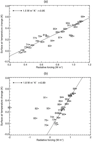
Figure 4. Relationship between annual-mean radiative forcing and surface air temperature anomaly

DTallfrom the ensemble mean of the HadCM3 all-forcings experiments for 1970 – 1999. Each point is

labeled with its year. (a) DTall is plotted against anthropogenic forcing FGA. The line is obtained by

ordinary least squares regression ofDTGAagainstFGA(the first method in the text). (b)DTallis plotted

against the sum of radiative forcingsFall. The line is obtained by ordinary least squares regression of

DTallandFallseparately against time (the second method in the text). In both cases the fits excluded years

strongly affected by volcanoes, which are those indicated by crosses; those included in the fits are indicated by asterisks.

[23] Since our interest is in the longer timescales, we

exclude the years strongly affected by volcanoes (the ‘‘volcano’’ years) from the calculation, identifying them as those in which the volcanic forcing has a magnitude exceeding 0.5 W m2. This is an ad-hoc criterion to remove the points that lie far off a linear relationship. However, the volcanic forcing is not zero in the other years. To obtain an estimate ofrunder these circumstances, we have tried three

methods, in all cases excluding the volcano years. 3.3.1. Ordinary Least Squares Regression of_DTall AgainstFGA

[24] The first method is to disregard the natural forcing

altogether, and regress DTall against the anthropogenic

forcing FGA as before (Figure 4a and ‘‘ModelTallv FGA’’

in Table 2). We treat the solar forcing like the volcanic because its dominant variation is likewise not monotonic, but periodic, on the 11-year solar cycle. We assume that such forcings do not affect DTon decadal timescales. The results of the regression are not significantly different from those usingTGA, because in these HadCM3 experiments the

overall warming in the 20th century, and its trend since 1970, are similar with and without natural forcing [see Gregory et al., 2006, their Figure 2], consistent with the assumption that natural forcings have little long-term effect. This is not surprising given their small average magnitude and trends (Figure 2). The standard deviation of unforced variability estimated from the residuals is about 0.12 K, as from the regression againstFGA. This equals the interannual

standard deviation of DT in the HadCM3 control run, in which forcing is constant, so only the unforced internal variability is present. The equality indicates that short-period fluctuation in the natural forcing has little effect onDT. 3.3.2. Ratio of Rates of Change of DTallandFall

[25] The second method takes natural forcing into

account but assumes that it affects only the trend in DT, not its interannual fluctuations. This method makes use of additional information about time-dependence, which is not exploited by regression. During recent decades, excluding the volcano years, the time series of bothDTandFallcan be

reasonably well fitted by linear functions of timeti.e.,DT= aT+bTtandFall=aF+bFt. For 1970 – 1999, the correlation coefficients with time ofDT in individual experiments are 0.8 – 0.9, of ensemble-mean DT 0.95, and of Fall 0.88.

Linear time-dependence is not a good approximation for the twentieth century as a whole, so we do not use this method for the entire period. The coefficients of the time-dependence can be estimated by OLS regression, because the independent variable in each case is time, in which there is no uncertainty. If both Fall and DT depend linearly on

time, they must have a linear relationship with each other:

Fall¼aFþbFt¼aFþbFðDTaTÞ=bT

¼ðaFaTbF=bTÞ þðbF=bTÞDT;

i.e., the linear relationship implied betweenFallandDThas

slope r= bF/bT, the ratio of the rates of change ofFalland

DT(Figure 4b, and ‘‘ModelbF/bT’’ in Table 2).

[26] The results for rfrom this rate-ratio method (1.8 +

0.4 – 0.4 W m2K1for the ensemble mean in 1970 – 1999) are larger than from the OLS regression. This is because of the difference in the forcing time series, not the different

method. If we apply the rate – ratio method to obtainrfrom

DTallandFGA, we obtain the same results as we did by OLS

regression ofDTallagainstFGA. It arises becauseFallhas a

greater upward trend thanFGA, owing (in the HadCM3 time

series) to an increase in solar forcing in the 1970s, and an increase in volcanic forcing i.e., a reduction in negative forcing in the late 1990s. Note that this increase comes only from the years with weak or no volcanic forcing, since the years strongly affected by volcanoes have been entirely excluded, possibly giving a biased estimate of the natural forcing trend.

[27] The uncertainty on r is estimated using a Monte

Carlo technique with the uncertainties onbTandbFfrom the separate regressions. (BecausebF/bTis nonlinear inbT, the confidence interval is not symmetrical.) The uncertainty is larger than from the OLS regression against FGA(the first

method) because the short-period fluctuations inFallmake

its trendbFrelatively uncertain. If these fluctuations have an effect onTall, part of the uncertainty inbTis correlated with uncertainty in bF; ignoring this means the uncertainty in their ratio is overestimated. However, the evidence from the first method is that such an effect must be small.

3.3.3. Total Least Squares Regression ofDTallAgainst

Fall

[28] Because of the fluctuations in Fall, we cannot use

what might appear to be the obvious method of OLS regression of Tall against Fall. The fluctuations represent

an uncertainty inFall, which means that OLS regression is

inapplicable [cf.Spencer and Braswell, 2008], as it assumes there is no uncertainty in the independent variable. Given an a priori estimate of this uncertainty, we could use the modified method, called ‘‘total least squares regression’’ (TLS) by workers in optimal climate fingerprinting, which allows for uncertainty in both variables. We have tried this method too, employing software from the Goddard Space Flight Center IDL Astronomy User’s Library that imple-ments the algorithm described byPress et al. [1992, their section 15.3 on straight line data with errors in both coordinates]. As estimates of the independent uncertainties inTallandFall, we used the standard deviations derived from

the residuals in their separate regressions of Tall and Fall

against time.

[29] This TLS method gives very similar results (not

shown) to the rate – ratio method (in fact they are the same for 1970 – 1999 to one decimal place), but it involves additional assumptions that are doubtful. First, it assumes that the same relation Fall = rDTall applies to interannual

variability as to the longer-term trend; this is certainly not the case in the volcano years, and may not be correct for other years, given the lack of evidence for correlation of interannual variability between Tall and Fall. Second, it

assumes that the uncertainty inFallis normally distributed,

which is not true because the volcanic forcing has a skewed distribution, with a longer negative tail. Because these reservations make the TLS method less robust, without yielding a reduction in uncertainty in the results, we prefer the rate-ratio method to the TLS method.

3.4. Summary of Results From HadCM3 Simulations of the Past

[30] From the HadCM3 results, we conclude that the

anthropogenic forcing in the twentieth century and for the idealized future 1% increase of CO2 from which TCR is

evaluated. It is obvious that the strong but short-lived forcing from volcanoes does not affect DT in the same way as anthropogenic forcing, but it is unclear what effect natural forcings have on the trend ofDT. If we assume that their trend on multidecadal timescales affects the trend of

DT, the climate resistance accounting for natural forcing in recent decades but excluding years with strong volcanic forcing is about 20% higher than for anthropogenic forcing alone (i.e., the ratio of r with natural forcing included to rwithout taking natural forcing into account). However, the

exclusion of volcano years may bias this result. We there-fore prefer the estimate without natural forcing, but note this issue as a systematic uncertainty.

4. Climate Resistance From Observed Past Changes

[31] Having shown that the TCR of HadCM3 can be

evaluated from its simulation of past changes, we next apply the same methods to estimates of past changes in the real world. Global average surface air temperature change dur-ing the last century is a relatively well-observed quantity. We use the time series derived by the Met Office and the University of East Anglia [HadCRUT3; Brohan et al., 2006]. As well as the scatter due to internal climatic variability, individual years have some random measure-ment and sampling error. In recent decades this has a standard deviation of 0.037 K [Brohan et al., 2006, their Figure 12].

[32] Estimates of past radiative forcing have considerable

uncertainty, despite improvements in recent years [Forster et al., 2007]. We show time series in Figure 5 of median estimates of the forcings. Long-lived greenhouse-gas forc-ings are derived from ice core, firn and in-situ measurements from a variety of sources [see Forster et al., 2007]. Solar forcings are by Wang [2005]. Aerosol forcings are

derived from the HadGEM1 AOGCM by Forster and Taylor [2006] and include a component due to land-use changes. The HadGEM1 model was chosen as it included absorbing aerosol species and its total aerosol forcing in 2005 matched the best estimate of the IPCC WG1 AR4 [see Forster et al., 2007]. Volcanic and ozone forcings are by Myhre et al.[2001], scaled to match the IPCC WG1 AR4 estimate in 2005, assuming no change in forcing during 2000 – 2005.

4.1. Climate Resistance From OLS and Rate-Ratio Methods

[33] The uncertainty in the anthropogenic forcing is

systematic, i.e., it means that any of the terms might be consistently over- or underestimated, rather implying ran-dom errors in individual years. Hence, as in the model, we can use OLS regression ofDTagainstFGA, which implicitly

assumes a uniform prior distribution for the dependent variableDT, i.e., all values are equiprobable in the absence of knowledge. Since the purpose is to evaluate DT for a given forcing, this choice of prior is consistent with the suggestion ofFrame et al.[2005].

[34] Excluding years strongly affected by volcanoes by

the same criterion as in the model, we evaluaterfor the three

time periods (Figure 6a, and ‘‘RealT v FGA’’ in Table 2). For

recent decades,rin the real world (2.1 + 0.4 – 0.3 W m2K1

for 1970 – 2006) is a little larger than in HadCM3. (The uncertainty is not symmetrical becauseris the reciprocal of

the regression slope.) The correlation coefficients are high, and the statistical uncertainties onrare smaller for longer

time periods.

[35] As in the model, we compare this with r from the

ratio of the slopes of Fall andT, excluding volcano years,

separately regressed against time, in order to take into account the trend of the natural forcing (Figure 6b, and ‘‘Real bF/bT’’ in Table 2). Again, as in the model, the resistance from this method (2.5 + 0.5 – 0.4 W m2 K1 for 1970 – 2006) is larger than from OLS regression ofDT Figure 5. Median estimates of real-world radiative forcings relative to 1850. Anthropogenic forcing is

the sum of forcings from greenhouse gases and anthropogenic aerosol.

against FGA, which we prefer, for reasons summarized in

section 3.4.

4.2. Uncertainty From Forcing

[36] The systematic uncertainty in FGA gives rise to

systematic uncertainty in r in addition to the statistical

uncertainty from unforced variability. The largest systematic uncertainty in FGA is associated with the poorly known

anthropogenic aerosol forcing FA. During the twentieth

century as a whole FA is temporally anticorrelated with

the greenhouse-gas forcingFG(Figure 5). If we

underesti-mate the magnitude ofFA, we will overestimate the increas-ing tendency ofFG+FA, which will reduce the fitted slope

in the regression of DT versus FGA, and hence bias r

upward. Fingerprinting studies can distinguish better be-tween the effects of FG andFA by considering the spatial patterns than we can do here by using only global averages [Stott et al., 2006].

[37] We can minimize the influence of the uncertainty in

FAby considering a period when it is changing least rapidly

Figure 6. Relationship between annual-mean estimated real-world radiative forcing and observed surface air temperature anomalyDTfor 1970 – 2006. Each point is labeled with its year. (a)DTis plotted against anthropogenic forcing FGA. The line is obtained by ordinary least squares regression of DT

againstFGA(the first method in the text). (b)DTis plotted against the sum of radiative forcingsFall. The

line is obtained by ordinary least squares regression ofDTandFallseparately against time (the rate-ratio

[Forster and Gregory, 2006]. That suggests restricting our attention to recent decades [Myhre et al., 2001, and Figure 5]. In Table 2 we show the results of regression against FG (‘‘Real T v FG’’). The comparison with the

results for FGAconfirms that omitting FAleads to largerr

for 1900 – 2006, during which periodFAchanged

substan-tially, but that results for 1970 – 2006 and 1980 – 2006 are insensitive toFA. Henceforth, we prefer to use 1970 – 2006 rather than 1980 – 2006 since the longer of these periods gives smaller statistical uncertainty in r. Forster et al.

[2007] give a median estimate of FA = 1.3 W m2 at

2005, with a 5 – 95% range of0.5 to2.2 W m2. If we assume the fractional uncertainty to be time-independent and scaleFA(t) by factors within this range,rfor 1970 – 2006 is

unaffected to two significant figures. Consequently we do not include an allowance for aerosol uncertainty in our results. However, we note that any time-dependent bias in the aerosol forcing would introduce a systematic error inr.

[38] Most of FG is due to long-lived greenhouse gases,

whose forcing has an uncertainty of 10% [Forster et al., 2007, their Table 2.12]. Forcing by ozone, both tropospheric and stratospheric, is smaller, but with a larger fractional uncertainty. During the twentieth century, ozone forcing was a reasonably constant fraction (9 – 14%) ofFG. Therefore we

account for the ozone forcing uncertainty as a constant fraction of FG, and we estimate that it increases the

uncertainty on FG to 13%, by reference to Forster et al.

[2007]. We combine this 13% systematic uncertainty on

r with the statistical uncertainty on r from the OLS

regression, and obtain r = 2.1 + 0.5 – 0.4 W m2 K1

(for 1970 – 2006).

[39] Since uncertainty in FA is disregarded, and

uncer-tainty inFGis common toF2andr, we can omit forcing

uncertainty in converting rto TCR. Our r= 2.1 + 0.4

0.3 W m2K1implies a 5 – 95% range for TCR =F2/r

in the real world of 1.5 – 2.1 K. This range is narrower than and lies within CMIP3 range of 1.2 – 2.4 K [Meehl et al., 2007].

4.3. Effect of Longer-Period Unforced Variability [40] The statistical uncertainty on the slope from OLS

regression ofDTagainstFGAreflects the effect of unforced

variability on DTon timescales which can be adequately sampled by the length of the time series used. However, unforced variability on longer timescales is not included. For instance, some or all of the trend inDTduring 1970 – 2006 might be due to internally generated climate variabil-ity on multidecadal timescales, rather than being caused by the forcing. This is the reason why the uncertainty from the ensemble mean in section 3 (Table 2) is greater than from the ensemble members, which have a spread arising from longer-period unforced variability. We cannot assess such variability from the observedDT, since we have only one realization of the real world. This problem is related to that of ‘‘detection’’ of climate change, i.e., deciding statistically whether the observed DT time series is consistent with unforced variability. It becomes more severe the shorter the observational record used, because the unforced variability becomes relatively larger. For example,Chylek et al.[2007] evaluateafromDTover the last decade by assuming it is

entirely a forced response; we suggest that there is substan-tial uncertainty in the results from such a short period due to unforced variability.

[41] This problem can only be addressed quantitatively by

using AOGCM control runs to assess the effect of variabil-ity on longer timescales. To do this, we use DT recon-structed from the OLS regression line of observed DT againstFGA, i.e., remove the temporal variability, generate

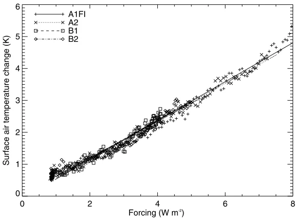
a set of realizations with synthetic temporal variability by adding randomly selected portions from CMIP3 AOGCM control runs to the reconstructed time series, and evaluate Figure 7. Annual-mean global-mean surface air temperature changeDTand radiative forcingF, with

respect to steady state in the late nineteenth century, simulated for the twenty-first century using the HadCM3 AOGCM under the four SRES marker scenarios indicated. For each scenario, a regression line has been plotted.

the distribution ofrfrom fitting the realizations. We carried

out this procedure using 19 different control runs. We also included randomly generated synthetic measurement and sampling uncertainty of the size estimated for the HadCRUT3 DT time series, but this has negligible effect by comparison with the variability from the control runs. The TCR range estimated from the real world is widened by allowing for this longer-period variability. However, the AOGCMs differ considerably regarding the magnitude of the effect. For instance, for standard deviations of trends over a period of the length of 1970 – 2006, CCCma CGCM3.1(T47) has 0.14 K century1, UKMO-HadCM3 0.30 and GFDL-CM2.1 0.49. In these cases, the TCR range is 1.5 – 2.1 K (not significantly widened), 1.3 – 2.3 K and 1.1 – 2.4 K respectively. It is notable that the last two are similar to the CMIP3 range, and that the means of both CMIP3 and our ranges are 1.8 K.

5. TCR and Equilibrium Climate Sensitivity [42] The equilibrium climate sensitivity DT2 = F2/a

is the warming in a steady state under 2CO2, as discussed

in section 1. Meehl et al. [2007] report that the 5 – 95% range of equilibrium climate sensitivity in CMIP3 models is 2.1 – 4.4 K. Over the last three decades, a lot of attention has been given to DT2 but it is still relatively poorly con-strained. A number of studies examined by Hegerl et al. [2007] and summarized by Meehl et al.[2007] (Box 10.2) have set observational constraints, but these are fairly weak, especially on the upper bound. That raises the question of why our observational constraint on the TCR is by contrast rather strong.

[43] Observational estimates of DT2 are, in effect,

attempting to deduce the climate feedback parameter a

from DT(t) in nonequilibrium states, when DT = F/(a + k) and a = (F N)/DT. There are three reasons why

uncertainty is larger in observational estimates ofDT2than

in our estimate of TCR.

[44] First, F is poorly known. This is the dominant

uncertainty if climate change relative to the preindustrial state is considered [Gregory et al., 2002] because of the aerosol forcing uncertainty, to which we have limited our exposure by our choice of time period (section 3.3).

[45] Second, ifDT2is large andasmall, such thatak,

then DT is insensitive to a. In this situation, N F; the

forcing is mostly being taken up by the ocean, climate feedback is making only a small contribution to resisting climate change, and it is hard to quantify a from this

contribution. That is why the upper bound of DT2 is

particularly uncertain. Another expression of this is the nonlinear relation between TCR and DT2:

TCR_¼ F2 aþk¼

F2

F2=DT2

ð Þ þk¼

DT2 1_þðkDT2=F2Þ

:

For smallDT2, TCR’DT2, but forDT2! 1, TCR! F2/k, i.e., independent of DT2. This is illustrated from

model results byKnutti et al.[2005, Figure 3a] andMeehl et al.[2007, Figure 10.25a], showing how TCR tends to level off for large DT2. For large DT2, even with a small uncertainty in TCR andr, there can be a large uncertainty in

DT2anda.

[46] Third, to extractafroma+krequires a knowledge

ofN, to obtaink. This can be evaluated from heat storage in

the ocean [Gregory et al., 2002;Forest et al., 2006] or the TOA radiative flux [Forster and Gregory, 2006], but in either case it is rather uncertain from observations. More-over, there is internal variability in N, as discussed in section 3.2, which increases the uncertainty in the evalua-tion ofk. When we evaluater=a+k, however, we do not

need a knowledge of N, because we are quantifying the overall climate response, rather than climate feedback or ocean heat uptake separately. Consistency with observed

DT in effect requires some cancellation of uncertainty betweenaandk[cf.Knutti and Tomassini, 2008].

6. Projections of Future Temperature Change 6.1. Scenario Dependence of Climate Resistance

[47] When we first introducedr = a+ k, we remarked

that we expectedF=rDTwith constantronly to apply for

scenarios of fairly steadily increasing forcing, because the approximation of constant k would otherwise be

inade-quate. Moreover, for scenarios with a slower rate of increase ofF, the climate system at any time will be nearer the steady stateF=aDT, sorwill be smaller.

[48] We can test the approximation of a constant

scenario-independentrfor projections of the twenty-first century in

simulations following various SRES emissions scenarios [Nakic´enovic´ et al., 2000] made with HadCM3 [Johns et al., 2003], using theDTandFdiagnosed from the model. The SRES scenarios give a range of increase in F over the twenty-first century (figures from the simple climate model ofCubasch et al.[2001], Appendix II.3 of the report) which would be achieved by rates of CO2 increase alone of

between 0.5% and 1.5% compounded per year, bracketing the idealized 1% scenario. The HadCM3 experiments show a scenario-independent linear relationship betweenDTand F (Figure 7). The relationship is not perfect because of variability on all timescales generated internally by the climate system. Nonetheless, the correlation coefficients are at least 0.98. The climate resistance r obtained from

OLS regression of DTagainst F is 1.6 – 1.8 W m2 K1, depending a little on scenario, but similar to r = 1.6 ±

0.1 W m2 K1 calculated from the 1% experiment. [49] Unfortunately radiative forcings from SRES

scenar-ios have not generally been diagnosed in AOGCMs, so we cannot present results similar to Figure 7 from other AOGCMs.Forster and Taylor[2006] estimated the forcing for SRES A1B in several models, but their method depends on the assumption thatain each model is constant in time

and not affected by the scenario, so the results they obtain are not entirely independent of the hypothesis we wish to test.

[50] However, using CMIP3 results for a wider range of

AOGCMs we can consider the ratio Ra/bDTa(t)/DTb(t) for pairs of SRES scenarios aandb. Ifris a constant, or

depends only on time, in any given modelRa/b(t) = Fa(t)/

Fb(t). If different models use the same forcings Fa(t) and Fb(t),Ra/b(t) will be model-independent.Meehl et al.[2007]

tuned a simple climate model to replicate the results of 19 AOGCMs from the CMIP3 database for SRES scenarios B1, A1B and A2. For any pair of SRES scenarios,Ra/b(t) is

scenarios available from the AOGCMs, Ra/b(t) has a

sub-stantial spread over models, which is likely to be due to model dependence in F(t). However, the AOGCM-mean Ra/b(t) is very close toRa/b(t) from the simple model, giving

some evidence for the scenario independence of climate resistance.Meehl et al.[2007] andKnutti et al.[2008] used this finding to estimate the AOGCM-meanDTa(t) for SRES scenarios for which the AOGCMs had not been run by scaling the AOGCM-mean DTA1B according to DTa(t) =

DTA1B(t) Ra/A1B(t) with Ra/A1B(t) from the simple climate

model.

[51] Stouffer and Manabe [1999] carried out a set of

experiments with the GFDL_R15_a AOGCM in which they applied rates of CO2 increase of between 0.25% and 4%

compounded per year, a much broader range than encom-passed by the SRES scenarios. Although all their experi-ments exhibit good linear relationships (their Figure 5), they show a substantial scenario dependence in r (calculated

from their Table 2), which varies between 1.4 W m2K1 for 0.25% and 2.5 W m2 K1 for 4%. It is smaller for lower rates, as expected. However, its variation between the 1% scenario (1.7 W m2 K1) and the 2% scenario (2.1 W m2K1) is only ±10%, while in HadCM3, the 2% scenario results inr= 1.8 ± 0.1 W m2K1, only slightly

larger than for the 1% scenario. Hence we consider that a scenario-independent ris an acceptable approximation for

SRES and other scenarios of practical interest for the twenty-first century. During 1970 – 2006 the real-world anthropogenic forcing FGA(t) had a rate of increase

equiv-alent to CO2 alone rising at 0.7% compounded per year.

Since this is within the SRES range, it supports the use of data from 1970 – 2006 to obtain a value forrappropriate for

the twenty-first century.

6.2. Projections for SRES Scenarios Using Climate Resistance

[52] IfF=rDTholds, we can userto make projections

of DT given F. For example, under emissions scenario SRES A1B the best estimate of the difference in FG between 2095 and 1990 is +4.3 and in FA +0.6 W m2

(also positive because aerosol forcing is projected to become less negative during the century). We assume that the projections of the contributions to the forcing have the same fractional uncertainties as their present-day estimates, namely forFGa normal distribution with a 5 – 95% range of

±13%, and forFAfollowing the probability density function

fromBoucher and Haywood [2001],Haywood and Schulz [2007] andForster et al.[2007]. Combining these by Monte Carlo sampling gives a 5 – 95% range of 4.4 – 5.5 W m2for FGA.

[53] Again using a Monte Carlo, we calculateFGA/rwith rfrom the OLS regression in section 4. The uncertainty on rincludes a contribution from the systematic uncertainty in

past FG, which is correlated with the uncertainty in future

FG, and these correlated uncertainties largely compensate.

In evaluating r and the TCR (section 2.1), we decided to

omit from consideration the possible induced cloud forcing of CO2 discussed by Gregory and Webb [2008] and

Andrews and Forster [2008]. Since CO2 is the dominant

contribution toFG, and provided this effect multipliesFGby

a constant ratio, it likewise will largely cancel out in the projections. BecausejF projected to increase andjFAj

to decline, their ratio changes with time. If the ratio were constant, the forcing uncertainty would cancel out entirely in the projections ofDT [Allen et al., 2000].

[54] The 5 – 95% range forDTfrom 1990 to 2095 is 2.0 –

2.8 K, which lies within and is narrower than the 5 – 95% range of projections from a set of 19 CMIP3 AOGCMs, from which we obtain 1.9 – 3.4 K (treating the models as normally distributed) for the difference in mean DT from 1980 – 1999 to 2090 – 2099. Enlarging the uncertainty onr

to take account of low, medium and high estimates for multidecadal unforced variability, following section 4.3, our projected range widens to 2.0 – 2.9 K, 1.7 – 3.1 K and 1.5 – 3.2 K respectively. These ranges are narrower than the likely range of 1.7 – 4.4 K from the assessment of Meehl et al.[2007] whose higher upper bound in particular reflects uncertainty in carbon cycle feedbacks that cannot be con-strained from the past (section 7 andKnutti et al.[2008]).

6.3. Time-Dependence of Climate Resistance

[55] As we saw in section 2.1, F / DT is a good

approximation in the 70 years of the 1% CO2experiments

up to 2CO2. However, deviations become apparent as the

forcing continues to rise. After a further 70 years, the scenario reaches 4 CO2. The increase in F, and hence

inDT, should be the same as in the first 70 years, i.e., the TCR. In fact, the warming during the second 70 years is greater in all the AOGCMs considered (Table 1). Examining N and F N shows that both k and a tend to decrease

(climate sensitivity rises, ocean heat uptake efficiency declines). (We calculate DT from 20-year means. For the first 70 years it is the mean for years 61 – 80. For the second 70 we use the difference between years 121 – 140 and 51 – 70; we cannot Centre a 20-year mean on year 140, since the 1% increase ends at year 140 in these experiments.) If the real world behaves qualitatively like this, projections made by scaling the TCR will tend to be underestimates; this is a possible explanation for our projections for A1B being lower than the AOGCM results. The underestimate would become more severe for projections further into the future, as the forcing rises. We note that in HadCM3 under SRES A1FI, the scenario with the strongest forcing, there is a tendency forDTto lie above the linear relationship in the 2090s (Figure 7).

7. Comparison With Optimal Fingerprinting [56] In effect, this method of estimatingDTfor the future

fromrfor the past is similar to scaling up the observed past

DTby the ratio of future forcing to past forcing, i.e.,DTf= Ff/FpDTp(f andpfor ‘‘future’’ and ‘‘past’’), which holds for constant r. A related idea has been employed by Stott and Kettleborough [2002] and Stott et al. [2006] in their observationally constrained projections, in which optimal fingerprinting methods (described by, e.g., IDAG [2005]) are used to estimate a factor by which an AOGCM simulation of the past should be scaled to agree with observations, to correct for errors in the modeled forcing and response. The same factor, with its uncertainty, is used to scale the AOGCM projection of the future, i.e., assuming that the fractional error inDTsimulated by the AOGCM is time-independent.

[57] Allen et al. [2000] supported this assumption by

considering the relationship between the temperature changes DT1 and DT2 at two times (with respect to an

initial steady stateDT= 0) as simulated by a simple climate model for a range of a. Their ‘‘transfer function’’ (their

Figure 2) is in effect a plot of DT2 against DT1 as a is

varied. They find it to be a straight line. A straight line with slope F2/F1 is expected if DT / F. Their result hence

indicates that F / D T is a good approximation for their simple climate model. Its use to support optimal finger-printing assumes that AOGCMs behave in the same way.

[58] Kettleborough et al.[2007] further investigated the

applicability of this linear approximation using the simple climate model, and concluded that the nonlinearity of the transfer function has only a minor effect on the projections made by scaling AOGCM results for SRES scenarios. However, their results show that the scaling works better for some scenarios than others. The use of scaling factors from optimal fingerprinting must have some similar limi-tations to the assumption of constant climate resistance.

[59] Optimal fingerprinting is a more powerful technique

than our regression ofFagainstDTbecause it makes use of the spatiotemporal patterns of temperature change, not just the global mean. Furthermore, it derives separate scaling factors for individual forcing agents, such as greenhouse gases and anthropogenic aerosol, and therefore does not assume that the climate is equally responsive to all of them. On the other hand, the regression has the advantage of not depending on model simulations of climate change. It avoids the systematic uncertainty inherent in modeling by instead making the simple assumption that DT_/F. Apart from the dependence on scenario already discussed, this relationship will be inaccurate if climate feedbacks emerge in the future that have not been observed in the past, for instance from nonlinear increases in carbon release from the biosphere or rapid weakening of the Atlantic meridional overturning circulation. However, this limitation applies equally to scaling based on optimal fingerprinting or to any other method of constraining projections using obser-vations [Allen et al., 2000;Kettleborough et al., 2007].

8. Conclusions

[60] Observations and AOGCM simulations of

twentieth-century climate change, and AOGCM experiments with steadily increasing radiative forcing F, indicate a linear relationshipF=rDT, whereDTis the global mean surface

air temperature change and r a constant ‘‘climate

resis-tance’’. The latter is the sum of the climate feedback parameteraand the ocean heat uptake efficiencyk. In the

CMIP3 AOGCMs, these two parameters have substantial and uncorrelated uncertainty, with a being about twice as

large askon average. The climate resistance is related to the

transient climate response according tor=F2/TCR, where F2is the radiative forcing due to doubled CO2

concentra-tion. This relationship is the analogue for time-dependent climate change of the relationship a= F2/DT2between

the climate feedback parameter and the equilibrium climate sensitivity DT2. The observational constraint on the

cli-mate resistance is much stronger than on the clicli-mate feedback parameter.

[61] In the real and simulated past record, deviations from

the linear relationship F / DT occur in years strongly affected by volcanic forcing, to which DT responds com-paratively weakly; further analysis would be useful of the different character of response to forcing which is episodic rather than multidecadal. Disregarding any trend caused by natural forcing, we estimate from the data of 1970 – 2006 by ordinary linear least squares regression that the real-worldr= 1.7 – 2.6 W m2K1and the TCR is 1.5 – 2.1 K

(5 – 95% uncertainty ranges). This range does not allow for the possible contribution to the observed DT of longer-period unforced variability, which can only be estimated using AOGCMs. When we incorporate a midrange estimate of this variability, obtained from the HadCM3 AOGCM, the TCR range is enlarged to 1.3 – 2.3 K. making it comparable to the CMIP3 AOGCM range of 1.2 – 2.4 K. The similarity of these ranges is notable because they are obtained from completely independent methods. Our range is not based on climate-change simulations, but uses only the observedDT and estimated pastF.

[62] The systematic uncertainties in natural forcing and

anthropogenic aerosol forcing may not be fully reflected in our stated range. A partial but possibly biased attempt to account for natural forcings gives a value ofrabout 20%,

larger i.e., TCR about 20% smaller. Our range is similar to 1.5 – 2.8 K derived by Stott et al. [2006] by optimal fingerprinting (converted from their units of K century1), and to 1.1 – 2.3 K obtained byKnutti and Tomassini[2008] by applying constraints from observedDTand ocean heat uptake to a very large ensemble of simulations of the past and future made by varying parameters in a climate model of intermediate complexity. These methods use more infor-mation (the entire twentieth century, and geographical patterns of variables other than surface air temperature), so it may appear surprising that their results have no less uncertainty. One possible reason is the comparative insen-sitivity of our result to the large uncertainty in anthropo-genic aerosol forcing, which was relatively constant during the period concerned, and therefore did not affect the trend inDT. Moreover, the relationshipF=rDTsuggests that the

recent few decades, during which change has been largest, are most influential in the observational constraint onrand

TCR.

[63] The linear relationship could not be expected to hold

under all scenarios; in general, it should be a reasonable assumption for scenarios of fairly steadily increasing forc-ing, in which casekDTis an acceptable approximation for

ocean heat uptake. The value ofrhas some dependence on

the scenario, so our empirical r is applicable only to

scenarios with a rate of future forcing increase within a restricted range, similar to that of the recent past from which it was evaluated. UsingDT=F/r, we obtain projections for