Hierarchical Bayesian Inversion for the Point Source Moment Tensor: Method and Applications

(1)

Hierarchical Bayesian Inversion for the

Point Source Moment Tensor: Method

and Applications

Marija Musta´

c

A thesis submitted for the degree of

Doctor of Philosophy at

The Australian National University

(2)

c

(3)

Declaration

This thesis is an account of research undertaken between July 2012 and August 2016 at the Research School of Earth Sciences, College of Physical & Mathematical Sciences, The Australian National University, Canberra, Australia.

Except where acknowledged in the text, the material presented in this thesis is, to the best of my knowledge, original and has not been submitted in whole or part for a degree in any university.

Marija Musta´c March, 2017

(4)

(5)

Acknowledgements

Primarily, I would like to thank my supervisor Hrvoje Tkalˇci´c for his guidance and support during this PhD. He showed me the intriguing side of earthquakes, and had valuable advice in many aspects of my work, from data processing to discussions. His enthusiasm for research has always been motivating, his academic rigour forma-tive, his company enjoyable and the meals he prepared have been delicious. I also sincerely appreciate his support when I was struggling with personal issues.

I am also grateful to my advisors. Malcolm Sambridge for his insight into the world of Bayesian inversion, clarity and elegancy of his explanations, Brian Ken-nett for valuable discussions and ease with which he augmented my knowledge in seismology, and Phil Cummings for his knowledge of seismic sources.

Many others have contributed to this research in various ways. Chronologically, I would like to thank Olivier Coutant for assistance with theAXITRA code, Douglas S. Dreger, Andrea Chiang and Sierra Boyd at the University of California, Berke-ley for valuable discussions and assistance, Alexender Burky form UC San Diego for his contribution in analysis of The Geysers earthquakes, Keiko Kuge from The University of Tokyo for valuable discussions on volcanic earthquakes and being a lovely host in Japan, Junkee Rhie and Sang–Jun Lee from the Seoul National Uni-versity for the Earth structure models, discussions and an enjoyable time in Seoul, Chang–Soo Cho from KIGAM for the data, Seongryong Kim for his contribution in looking at the DPRK event, Christian Sippl and Roberto Benavente for casual discussions throughout the years. Last but not least, Maree Coldrick, Sherryl Klu-ver and Mary Hapel for assistance with the administrative issues, and the RSES IT team for timely assistance and support.

This research was supported by an Australian National University Research Scholarship and AE Ringwood Supplementary Scholarship, as well as the USA DoD/AFRL under grant no. FA9453-13-C-0268. This study makes use of the computer package Hyper–sweep which was made available with support from the Inversion Laboratory (ilab). Ilab is a program for construction and distribution of data inference software in the geosciences supported by AuScope Ltd, a non–profit organisation for Earth Science infrastructure funded by the Australian Federal Gov-ernment. Waveform data, metadata, or data products for this study were accessed through the Northern California Earthquake Data Center (NCEDC) or provided by

(6)

the Korea Institute of Geoscience and Mineral Resources (KIGAM).

(7)

Abstract

One of the most important aspects of seismology is explaining the generation of seismic waves during earthquakes. The first mathematical models of earthquakes involved shear faulting, where deformation of rocks surrounding the fault increases the stress level. When the stress across the fault exceeds the frictional resistance of the rocks, it causes rock fracturing and results in radiation of elastic waves. Over the years, a large number of earthquakes that cannot be explained only with shear faulting (i.e. a double–couple force system) have been observed. Hence, the mathe-matical model of seismic sources evolved into a seismic moment tensor (MT), which also includes isotropic and compensated linear vector dipole components. Although uncertainties in MT inversions are important for estimating solution robustness, they are rarely available. If earthquake location is simultaneously recovered, the problem becomes non–linear and uncertainties cannot be calculated in a simple manner. Furthermore, noise in the data can alter the waveform and cause spurious non–double–couple components.

In this thesis, I address these issues using Bayesian hierarchical inversion, a relatively novel technique in seismology. Its probabilistic approach gives an ensemble of solutions instead of just one best–fit solution, thus, it can be used to estimate MT uncertainties. The algorithm developed as a part of this thesis uses waveform data of regional earthquakes and explosions with moderate magnitudes to compute the centroid location and the seismic moment tensor. Including the source location as a parameter enables one to explore the errors introduced by source mislocation. The algorithm includes a sophisticated treatment of data noise. I utilise the pre–event noise to create an empirical noise covariance matrix, and include the level of noise as an unknown in the inversion. As a result, the model complexity is determined by the data themselves.

There are two major groups of events for which the Bayesian approach can be of great importance, and to which the algorithm has been applied. The first one is seismic events in complex geological environments, such as volcanic and geothermal areas. A significant number of these events are expected to have source processes that cannot be explained using only a double–couple, but require the full MT. The second group is man–made events such as explosions, where the algorithm can be valuable for nuclear proliferation. The feasibility of the approach is initially demonstrated on synthetic data contaminated with noise and it is shown that the

(8)

empirical covariance matrix improves the estimate of the location. This is followed by application to a well–studied earthquake from Long Valley caldera, a volcanic environment in California, where a statistically significant isotropic component of the source is confirmed without a trade–off with the compensated linear vector dipole component.

The method was further improved to include multiple noise parameters that de-termine the fit on each record, and in turn weight the stations’ contribution in the inversion. This inclusion proved to be justified by the data in synthetic experiments, and when applied to the same earthquake from Long Valley caldera. Subsequently, I have analysed several earthquakes from a geothermal field in California, The Gey-sers. The double–couple components of the sources agree well with the regional stress field, but the non–double–couple components show a variety of values.

(9)

List of Figures

1.1 Relation between displacement on the fault and equivalent body forces. Cracking and frictional sliding over a surface can be ap-proximated by a time–varying average displacement. The average displacement can then be replaced by a system of equivalent forces which produce the same motions outside the source region. Figure taken from Lay and Wallace (1995). . . 3 1.2 Representation of the elements of the moment tensor as weights for

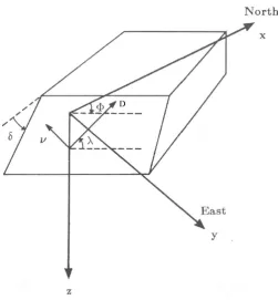
a set of dipoles and couples. Figure taken from Kennett (2009). . . . 5 1.3 Cartesian coordinate system describing the fault orientation. The

origin is in the epicentre. Strike angle φ is measured clockwise from north, dip angle δ from horizontal down and slip angle λ counter-clockwise from horizontal. D and ν are the slip vector and the fault normal, respectively. The figure is modified fromJost and Herrmann

(1989). . . 7

1.4 Components of the moment tensor from left to right: ISO, DC and CLVD; (a) Equivalent force systems. DC is shown as two linear dipoles in the top row and as couples which individually exert a torque in the bottom row. (b)P wave radiation patterns. The figure is taken fromJulian et al. (1998). . . 7 1.5 Elementary moment tensors used in the inversion (equal–area

projec-tion of the lower focal hemisphere). . . 10

2.1 Auto–correlations (for non–negative lags) of the three–component noise seismograms on different stations around the globe. Group one shows results for four stations in California (BKS, CMB, KCC and ORV), two stations in Australia (CTAO and ERAB), one in Japan (ERM) and one in north Russia (NRIL). Stations in Group two (BRVK in Kazakhstan, ESK in the United Kingdom, MBAR in Uganda and NNA in Peru) have more complex auto–correlations of the horizontal components. . . 30

(12)

2.2 (a) Auto–correlations of 15 noise series (three components of noise on five stations) and their average value. (b) The best–fit values of an exponential and two attenuated cosine functions for the aver-age auto–correlation. (c) Covariance matrices corresponding to the average auto–correlation (empirical) and the best–fit for the two pa-rameterisations. . . 32

2.3 Map of the region showing the earthquake location in Long Valley caldera (green star), location of real stations used in the inversions (red triangles) and synthetic stations added in the last synthetic ex-periment (blue triangles). The insert in the lower left corner shows the smaller caldera area. . . 33

2.4 Centroid locations for one thousand iterations in the outer Markov chain for the inversion of data without noise assuming a covariance matrix with two attenuated cosine functions. The average iteration number for each location determines its colour. Open circles show all proposed locations and full circles are the accepted ones. Symbol sizes are determined by the likelihood value (the 1% MAP locations are plotted with the largest circle, the next 9% with a smaller one, etc.). The black star represents the input location, while the green circle shows the MAP location. The first subplot shows locations in 3–D, and the other three subplots are cross sections through the MAP source location. . . 35

(13)

LIST OF FIGURES xiii

2.6 (a) The input mechanism (black) and MAP solutions obtained for data without noise assuming a diagonal (grey), exponential (blue) and two–attenuated–cosine (red) covariance matrix. (b) Synthetic data and seismograms from three MAP solutions, coloured in the same way as beachballs. (c) Lune source–type plots with solutions from all locations shown in light colours and the final ensemble shown in darker colours for the three inversions. The colours are as in the previous two plots; the star shows the input value. (d), (e) and (f) are the same for data with a low level of noise and (g), (h) and (i) for data with a high level of noise. . . 38

2.7 Similar to figure 2.5, but for inversions of synthetic data with a high level of noise using: (a–c) five stations and (d–f) ten stations. . . 39 2.8 (a) Input and recovered focal mechanisms for a synthetic experiment

with ten stations. (b) Three component seismograms. (c) The lune plots for all three assumptions of CD. For details see the caption of

figure 2.6. . . 41

2.9 Sampled centroid locations for real data from Long Valley caldera. For details see the caption of figure 2.4. . . 42

2.10 The double–couple part of the solutions for the LVC data, for details see the caption of figure 2.5. . . 43 2.11 Inversion results for the LVC data: (a) focal mechanisms, (b)

seismo-grams, (c) the lune plots. For details see the caption of figure 2.6. The green beachball in (a) and stars in (c) show the solution from

Minson and Dreger (2008). . . 44

3.1 (Grey) Auto–correlations of noise series on three seismogram compo-nents filtered between 20 and 50 s and (dashed black line) their fit using two attenuated cosine functions (cross–diagonal terms of the

Cn matrices defined in equation 3.1). (b) Covariance matrices Cn for

the horizontal and vertical components. . . 52

3.2 Flow diagram of the algorithm. The data covariance matrix and elementary seismograms are computed and the number of iterations determined prior to the inversion. Two Markov chains are used to sample the model space. For each location in the outer chain, six moment tensor parameters (a1 to a6) and the noise are sampled in

(14)

3.3 Map of the studied region with the LVC (black star) and The Gey-sers earthquake locations (white star), as well as stations used in the inversions of the LVC earthquake (black inverted triangles) and The Geysers earthquake (white inverted triangles). Station BKS was used in the analysis of both earthquakes. . . 55

3.4 (Grey) The logarithmic likelihood and (black) the BIC values for in-versions with (top) a diagonal, and (bottom) a two–attenuated–cosine covariance matrix for different numbers of noise hyperparameters in the inversion. BIC and likelihood values for two, three, and four noise parameters are averages from all inversions. . . 56

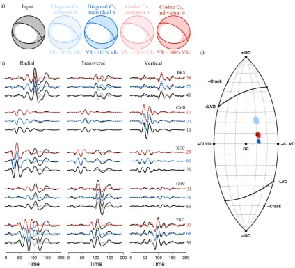
3.5 Comparison of solutions with different assumptions for CD. (a)

In-put mechanism and MAP solutions from inversions with a diagonal and a two–attenuated–cosine CD and one (common σ) and five

(in-dividual σ for each station) noise parameters. The numbers below beachballs show that most inversions have higher variance reduction (VR = 1−

R

(d−G(m))2

R

d2 ) than VR0, computed between the data with

and without noise. (b) (Grey) data without noise, (black) data with noise and synthetic seismograms from MAP solutions, coloured as in (a). Seismograms from inversions with multiple noise parameters are plotted with a dashed line. Numbers on the right hand side of the seismograms show the input level of noise (black) and the MAP values obtained in inversions with a diagonal (blue) and a two–attenuated– cosine (red) CD matrix for each station. (c) Lune source–type

di-agram showing the input mechanism (black star) and ensembles of solutions from the same four inversions, coloured as in (a). . . 58

3.6 (Grey) The logarithmic likelihood and (black) the BIC for the LVC earthquake, similar to figure 3.4. . . 59

3.7 (a) MAP solutions, (b) observed seismograms (black) and synthetic seismograms with added MAP noise values (blue for a diagonal CD

matrix and red for a two–attenuated–cosineCDmatrix), and (c) Lune

(15)

LIST OF FIGURES xv

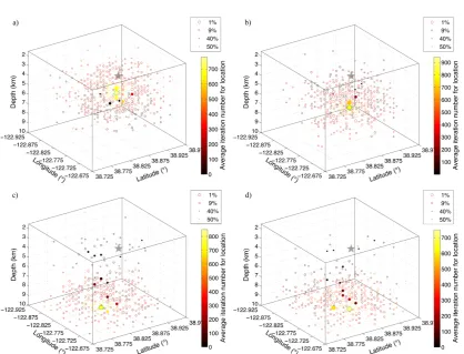
3.8 Centroid locations for 1000 iterations in the outer Markov chain for the inversion of Geysers data assuming a (a) diagonal covariance ma-trix and using one noise parameter, (b) diagonal covariance mama-trix and using five noise parameters (c) two–attenuated–cosine covariance matrix and using one noise parameter, (b) two–attenuated–cosine co-variance matrix and using five noise parameters. The average iter-ation number for each lociter-ation determines its colour. Open circles show all proposed locations and full circles are the accepted ones. Symbol sizes are determined by the likelihood value (the 1 per cent MAP locations are plotted with the largest circle, the next 9 per cent with a smaller one, etc.). The grey star represents the CNSS hypocentre location, while the green circle shows the MAP location. . 62

3.9 (a) Observed seismograms (black) and synthetic seismograms with added MAP noise values (blue for a diagonal CD matrix and red

for a two–attenuated–cosine CD matrix), (b) MAP solutions, and

(c) Lune source–type diagram for The Geysers earthquake ensemble solutions. The colour scheme for the ensemble solutions is given in (b). 63

4.1 Auto–correlations of horizontal and vertical component noise seismo-grams from two groups of stations in California. The dashed red and yellow lines are the average auto–correlation of a particular type, while the solid red and yellow lines are the two attenuated cosine fits. 69

4.2 Map of California showing the location of earthquakes in The Gey-sers region (white star) and stations used in the inversions (inverted triangles). Only one earthquake location is plotted because of their proximity on this map. Red inverted triangles are stations from group 1 and yellow inverted triangles are stations from group 2 in figure 4.1. Please note that data from different stations were used for different events. . . 70

(16)

4.4 (Top) Comparison of maximum a posteriori probability (MAP) so-lutions with different assumptions for the covariance matrix for the 18 Feb 2004 event: (Light blue) a diagonal CD and a common noise

parameter, (dark blue) a diagonal CD and multiple noise parameters

(light red) two–attenuated–cosineCDand a common noise parameter,

and (dark red) two–attenuated–cosineCD and multiple noise

param-eters. Numbers above beachballs show the percent of DC, CLVD and ISO components. (Bottom) Waveform data is shown in black and synthetic seismograms from the corresponding MAP solutions. Seis-mograms from inversions with multiple noise parameters are plotted with a dashed line. . . 72

4.5 Ensembles of solutions from the four inversions for the 2004 event, coloured as in figure 4.4 and shown on a lune source–type diagram. . 74

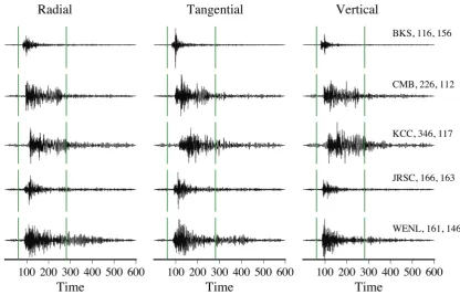
4.6 Velocity seismograms from ten stations used for the 24 Apr 2007 earthquake. The horizontal seismograms are rotated to radial and tangential components. Vertical green lines indicate the part of the waveform used for moment tensor inversion. The numbers next to station names are epicentral distances in kilometres and azimuths in degrees. . . 75

4.7 (Top) MAP solutions for the 24 Apr 2007 event from four inversions with DC, CLVD and ISO percents indicated above, coloured as in figure 4.4. (Bottom) Waveform data and synthetic seismograms cor-responding to the solutions above. . . 76

4.8 Ensembles of solutions from the four inversions for the 24 Apr 2007 event, coloured as in figure 4.4 and shown on a lune source–type diagram. . . 77

4.9 Velocity seismograms from ten stations used for the 11 Jan 2014 earthquake. The horizontal seismograms are rotated to radial and tangential components. Vertical green lines indicate the part of the waveform used for moment tensor inversion. The numbers next to station names are epicentral distances in kilometres and azimuths in degrees. . . 78

(17)

LIST OF FIGURES xvii

4.11 Ensembles of solutions from the four inversions for the 11 Jan 2014 event, coloured as in figure 4.4 and shown on a lune source–type diagram. . . 80

4.12 Evidence values for the inversions of the 20 Oct 2006 earthquake, normalised with the highest value. The colours are as in the previous figures (light blue for the inversion with a diagonalCD and a common

noise parameter, dark blue for multiple noise parameters, light red for the inversion with the empiricalCD and a common noise parameter,

dark red for multiple noise parameters). . . 81

4.13 Evidence values for the inversions of the 2004 earthquake, normalised with the highest value, coloured as in figure 4.12. . . 82

4.14 Evidence values for the inversions of the 24 Apr 2007 earthquake, normalised with the highest value, coloured as in figure 4.12. . . 82

5.1 Map of the region showing (red star) the event location and (black triangles) stations used in the inversion. . . 86

5.2 Displacement seismograms from seven stations used in this study. The presence of SH and Love waves can be observed on the tangential component. Vertical green lines indicate the part of the waveform used for moment tensor inversion. The numbers next to station names are epicentral distances in kilometres and azimuths in degrees. . . 88

5.3 Displacement seismograms filtered between 12.5 and 25 s. . . 89

5.4 Three Earth structure models used to create Green’s functions. vP

and vS are P and S wave velocities, respectively (Lee and Rhie, 2016). 90

5.5 Linear inversion result for the average model (shown in figure 5.4), together with (black) observed and (grey dashed) synthetic seismo-grams. . . 91

5.6 Linear inversion result for the composite model (explained above), to-gether with (black) observed and (grey dahsed) synthetic seismograms. 93

5.7 (Top) Input mechanism and the synthetic test result with allowed time shifts. (Bottom) Synthetic data is shown in black and seismo-grams from the obtained solution in grey. . . 94

(18)

5.9 (Top) Comparison of MAP solutions with (light blue) a single and (dark blue) individual noise parameters for the inversion with the average model Green’s functions. The numbers above beachballs show the percents of the DC, CLVD and ISO components, in that order. (Bottom) Waveform data and synthetic seismograms from the MAP solution. . . 97 5.10 (Top) Comparison of MAP solutions with (light blue) a single and

(dark blue) individual noise parameters for the inversion with the composite model Green’s functions. The numbers above beachballs show the percents of the DC, CLVD and ISO components, in that order. (Bottom) Waveform data and synthetic seismograms from the MAP solution. . . 98 5.11 Lune source–type diagrams showing solutions from inversions with

(left) the average and (right) the composite structure model Green’s functions. Solutions from (light blue circles) Bayesian inversions with a single noise parameters, (dark blue circles) Bayesian inversions with individual noise parameters for each station and (black diamonds) linear inversions are shown. . . 99 5.12 Evidence values from inversions with (light blue circles) Bayesian

(19)

List of Tables

2.1 Range of parameter values for data without noise, in degrees. Strike, dip and slip are the usual parameters defining the double–couple part of the solution, γ and δ are parameters from Tape and Tape (2012) that determine the amount of CLVD and isotropic components, re-spectively. Parameter γ can have values between -30◦ and 30◦ and δ

between -90◦ and 90◦. . . 36 2.2 Range of parameter values for data with ∼16% noise. For details see

table 2.1. . . 37 2.3 Range of parameter values for data with ∼65% noise. For details see

table 2.1. . . 40 2.4 Range of parameter values for an inversion that uses 10 stations with

∼65% noise. For details see table 2.1. . . 40 2.5 Range of parameter values for LVC data. For details see table 2.1. . . 44

4.1 Locations and moment magnitudes of earthquakes analysed in this study as reported by BSL. . . 69

5.1 Variance reduction values in percents for single station inversions with Green’s functions computed using models shown in figure 5.4. The maximum of those three values is in boldface font. . . 92

(20)

(21)

Chapter 1

Introduction

Earthquake generation was initially explained by shear faulting, from which quanti-tative descriptions evolved into detailed mapping of ruptures within rocks. The level of detail to which an earthquake source can be described depends on its dimensions and the data used to study it. Earthquakes whose dimensions are small compared to the wavelength of seismic waves can be sufficiently approximated by a point source, and their generation described using the seismic moment tensor (MT).

In addition to slip on a plane, the moment tensor can describe processes involv-ing a volume change and other non–shear phenomena. This is particularly impor-tant for earthquakes occurring in complex geological settings, such as volcanic and geothermal areas, mines and deep subduction zones. Due to its volumetric part, the moment tensor can also be used to study explosions, and applied in nuclear monitoring. Computation of the moment tensor, particularly in such complex and noisy environments, is still a delicate procedure due to underlying assumptions and noise in the data.

In this Chapter, we present some key concepts fundamental to studies of small and moderate size earthquakes, difficulties related to current techniques, and an inversion technique relatively new to geophysics that can address some of the diffi-culties. Firstly, in Section 1.1 we present the seismic sources, focus on the moment tensor, and critically evaluate its retrieval. Secondly, the fundamental concepts of Bayesian inversion are introduced in Section 1.2. The advantages of Bayesian frame-work are the ability to estimate parameter uncertainties and to account for noise in the data.

1.1 The seismic moment tensor

1.1.1 General description of seismic sources

Depending on the way seismic waves are excited, their sources are divided into inter-nal and exterinter-nal sources. Various exterinter-nal phenomena can act as a source, such as

(22)

meteorite impacts, wind and atmospheric pressure, ocean waves and tides or human impact (e.g. rocket launches, traffic, planes, railways). In most cases, seismology deals with sources internal to the solid Earth. They are more difficult to study an-alytically because the processes behind wave generation cannot be formulated in a simple manner. The common and best known internal sources are earthquake fault-ing, underground explosions, rapid phase changes and magma movements. Some sources, such as volcanic eruptions and landslides, are a combination of forces with both internal and external origin. When retrieving source properties, seismologists approximate true physical processes with models appropriate for the studied source and data used in the study. For example, finite fault models are adequate for large magnitude earthquakes, with complex ruptures and large source areas. For earth-quakes with small and moderate magnitudes, when long wavelength data is used, the point source is a sufficient approximation.

First mathematical models of earthquake sources involved shear faulting (Gilbert, 1884; Reid, 1910). Reid’s elastic rebound theory was a major breakthrough in seis-mology. It describes earthquakes as a result of rock fracturing caused by strain accumulation in a narrow region. This concept remains valid today. The strain accumulates in a narrow band near the fault as a consequence of tectonic plate movements, and increases the stress level. When the stress across the fault over-comes the material strength, its large proportion causes rock fracturing or dissipates through friction as heat. The remaining part is radiated as elastic waves and can be detected at the surface. Although direct observations of dislocations on the en-tire fault surface are not possible, the faulting process can be approximated by a time–varying average dislocation. The size of an earthquake can be expressed by its seismic moment M0 = µA ¯D, where µ is the shear modulus, A is the fault

(23)

§1.1 The seismic moment tensor 3

Figure 1.1: Relation between displacement on the fault and equivalent body forces.

Cracking and frictional sliding over a surface can be approximated by a time–varying average displacement. The average displacement can then be replaced by a system of equivalent forces which produce the same motions outside the source region. Figure taken from Lay and Wallace (1995).

1.1.2 Point sources and the moment tensor

A basic assumption in point source inversions is replacing the kinematic rupture process by a dynamically equivalent force system, using the representation theorem (Aki and Richards, 2002). Equivalent forces represent the difference between stress in the model and true physical stress, called the stress glut (Backus and Mulcahy, 1976). They produce the same seismic wave radiation pattern and consequently the same displacements on Earth’s surface, as the non–linear failure processes in the source region would. For convenience, the medium in which the forces act is usually considered to be linearly elastic, isotropic and homogeneous.

We can express the displacement ui in direction xi at any point x and time t

using the equivalent body force of density fj acting in xj direction in the source

region in the following manner

ui(x, t) =

Z

V

Gij(x,r, t)∗fj(r, t) dV . (1.1)

Summation over repeating indices is assumed, asterisk indicates temporal convolu-tion, and V is the source volume where fj are non–zero. Gij are components of

elastodynamic Green’s functions, which give a displacement field in directionxi due

to a unit impulse force acting in the direction xj. They depend on the source and

(24)

series around a reference point r=r0, called the centroid

Gij(x,r, t) = Gij(x,r0, t) +Gij,k(x,r0, t)(rk−r0k) +· · · (1.2)

and equation 1.1 becomes

ui(x, t) =Gij(x,r0, t)∗Fj(t) +Gij,k(x,r0, t)∗Mjk(t) +· · · (1.3)

It contains the total force exerted by the source

Fj(t) =

Z

V

fj(r, t) dV, (1.4)

which is usually neglected because the linear momentum is conserved in most pro-cesses. It needs to be included when the momentum is transferred between the source region and the rest of the Earth. This is the case with landslides, volcanic eruptions and unsteady fluid flow (Julian et al., 1998). Landslide modelling in-volves a block of mass M moving down an inclined surface. The equivalent force is -Mg sinθ, whereg is the acceleration of gravity and θ is the incline angle. Its direc-tion is parallel to the incline. Volcanic erupdirec-tions can excite seismic waves because the erupted material applies a net force to the Earth. This force can be expressed as S∆P, where S is the area of the volcanic vent and ∆P is the pressure difference between the volcano reservoir and the atmosphere. Another volcanic source process that can be modelled with a single force is unsteady fluid flow. If the magmatic fluid of density ρ flows in a volcanic conduit with acceleration a, it exerts a force

F=R_VρadV. However, it is not necessary to include the single force in most cases of seismic source modelling.

For waves whose wavelength is significantly longer than the source dimensions, the inversion can be linearised by omitting the higher order terms in equation 1.3 and we are left only with the second term containing derivatives of the Green’s functions Gij,k and elements of the moment tensor Mjk. Green’s functions’

deriva-tives with respect to the source coordinate rk are responses of elastic media to force

couples with arms in the k direction. Three force components and three possible arm directions give nine generalised couples (figure 1.2). The moment tensor has the form

Mjk(t) =

Z

V

(rk−r0k)fj(r, t) dV (1.5)

(25)

[image:25.595.207.453.100.360.2]

Figure 1.2: Representation of the elements of the moment tensor as weights for a set of

dipoles and couples. Figure taken from Kennett (2009).

x1 with arm in direction x2). Thus, equation 1.1 becomes

ui(t) =Gij,k∗Mjk (1.6)

Under the constraint that the force couples do not exert any net torque, the moment tensor is symmetric and has only six independent elements. This is true for various physical processes, such as shear faulting on a complex surface, faulting in an anisotropic or heterogeneous medium, tensile faulting and polymorphic phase transformations.

Decomposition of the moment tensor

To facilitate understanding of the moment tensor and its relation with true motions within the source, it is usually decomposed into an isotropic and a deviatoric part. The isotropic component Miso consists of the diagonal elements M11, M22 and M33,

which correspond to linear dipoles. It is proportional to the volume change ∆V that occurred in the process through the equation Miso = (M11+M22+M33)/3 = k∆V,

(26)

has incorrect equations for the full moment tensor inversion in Appendix V). The decomposition most commonly used comprises a double–couple and a compensated linear vector dipole (CLVD). Therefore, the aforementioned double–couple is in-cluded in the seismic moment tensor. When rotated by 45◦ to its principal axis, the double–couple consists of two linear dipoles of equal magnitude, but opposite signs, i.e. one of its eigenvalues is zero and the remaining two have equal magnitude, but opposite sign. As mentioned above, the double–couple is the equivalent force system for shear dislocations, for which the moment tensor components are given by

Mij =µA(Diνj+Djνi), (1.7)

where ν is the fault normal. The moment tensor components can be related to the geometry of the shear fracture (shown in figure 1.3) in the following way

Mxx =−M0(sinδcosλsin 2φ+ sin 2δsinλsin2φ) Myy =M0(sinδcosλsin 2φ−sin 2δsinλcos2φ) Mzz =M0(sin 2δsinλ) Mxy =M0(sinδcosλcos 2φ+ 0.5 sin 2δsinλsin 2φ) Mxz =M0(cosδcosλcosφ+ cos 2δsinλsinφ) Myz =M0(cosδcosλsinφ−cos 2δsinλcosφ),

(1.8)

where M0 is the total seismic moment,φ is the strike angle, δ is the dip angle and λ is the slip angle.

The remaining CLVD has eigenvalues in the ratio 1 : -1/2 : -1/2. It consists of a unit strength linear dipole and two half strength dipoles in a plane orthogonal to the first one. These three force systems (DC, CLVD and ISO) are shown in figure 1.4, together with their P wave radiation patterns. The complete moment tensor was first computed in a pioneering paper by Gilbert and Dziewonski (1975).

Physical processes involving non–double–couple sources

As previously mentioned, earthquakes with non–double–couple mechanisms mostly occur in volcanic and geothermal areas, deep subduction zones and mines. They can be theoretically explained by tensile faulting, geometrically complex shear faulting, heterogeneities or anisotropy in the medium, and polymorphic phase transformations (Julian et al., 1998). Now, we are going to discuss some physical processes that are modelled using the CLVD and/or isotropic components of the moment tensor.

(27)

[image:27.595.204.456.108.380.2]

Figure 1.3: Cartesian coordinate system describing the fault orientation. The origin is in

the epicentre. Strike angleφis measured clockwise from north, dip angleδfrom horizontal down and slip angle λcounterclockwise from horizontal. D and ν are the slip vector and the fault normal, respectively. The figure is modified fromJost and Herrmann (1989).

Figure 1.4: Components of the moment tensor from left to right: ISO, DC and CLVD; (a)

[image:27.595.189.477.481.692.2]

(28)

non–double–couple earthquakes in volcanic and tectonic regions. Tensile faulting is a mechanism where the slip vector is normal to the fault plane. This behaviour is restricted by compressive stress. It can occur when the pore fluid pressure lowers the effective principal stresses and cancels out a large part of the compressive stress caused by the lithostatic load. Another prerequisite is a small shear stress, or nearly equivalent principal stresses. Tensile faulting can be modelled with three orthogonal linear dipoles in the ratio (λ+ 2µ:λ:λ), where µand λ are the Lam´e parameters. This is equivalent to a combination of an isotropic source of moment (λ+ 2/3µ)A ¯D

and a CLVD of moment (4/3µ)A ¯D, where A is the total fault area and D¯ is the average displacement. The far–field P waves have first motions outward for all ob-servation directions (for an opening crack), with amplitudes largest in the direction normal to the fault. A shear and a tensile fault can intersect (Shimizu et al., 1987) and have sudden episodes of either opening or closing, with volume increases or decreases. This results in a moment tensor with all three components (DC, CLVD and ISO).

Another mechanism that involves non–double–couple components are rapid min-eral phase changes (e.g. Kirby et al., 1991). This process can explain deep earth-quakes, occurring in parts of the Earth where brittle behaviour of rocks is not expected. Many minerals are subjected to polymorphic phase changes at certain pressure and temperature conditions. Phase transformations can occur when slabs subduct into the mantle, in regions where denser mineral phases are stable. Changes in mantle structure at depths between about 410 and 660 km are attributed to phase changes, mostly involving the mineral olivine. If the phase change happens quickly, seismic waves are radiated and interpreted as earthquakes with isotropic components. However, phase transformations can occur in narrow zones and have double–couple mechanisms.

(29)

as a single event with a moment tensor representing a sum of the individual events. Even if they are both DC events, their sum can have non–DC components. Fault ge-ometries that allow earthquakes oriented in this way are mostly found in subducted slabs and mid–ocean ridge environment. Individual events can often be resolved by allowing the moment tensor elements to vary with time. Shearing on volcanic ring faults might require more complex, finite–source modelling (e.g. Fichtner and Tkalˇci´c, 2010).

1.1.3 Linear complete waveform moment tensor inversion

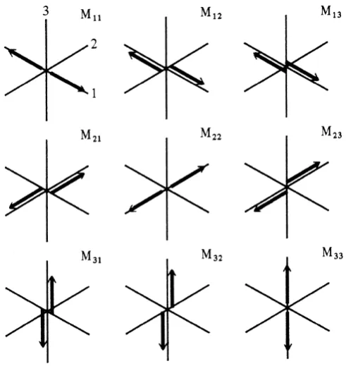
Moment tensor decomposition, presented in the previous section, is valuable when looking at the final result, but to calculate the moment tensor from measured displacements we decompose it in a different manner. We use the frequency– wavenumber code AXITRA (Bouchon, 1981; Cotton and Coutant, 1997), based on the approach of Kikuchi and Kanamori (1991), to create Green’s functions. The code convolves the Green’s functions’ derivatives with the following six elementary seismograms (their mechanisms are shown in figure 1.5)

M1 =



 

0 1 0 1 0 0 0 0 0

   M 2 ₌   

0 0 1 0 0 0 1 0 0

   M 3 ₌   

0 0 0 0 0 −1 0 −1 0



 

M4 ₌



 

−1 0 0 0 0 0 0 0 1

   M 5 ₌   

0 0 0 0 −1 0 0 0 1

   M 6 ₌   

1 0 0 0 1 0 0 0 1



 

(1.9)

This combination is particularly convenient for obtaining specific solutions using subsets of elementary moment tensors. TensorM6 _{is a purely isotropic source, while}

the remaining tensors M1 _to _M5 _{are five double–couples. Consequently, the subset} M1 _to _M5 _{corresponds to a deviatoric solution. Constraining its determinant to}

zero makes the mechanism a pure double–couple. In that case, the inversion is non–linear. The subset M1 _to_M3 _{gives a mechanism with a vertical nodal plane.}

The full moment tensor is a linear combination of elementary moment tensors, with coefficients an

(30)

Figure 1.5: Elementary moment tensors used in the inversion (equal–area projection of the lower focal hemisphere).

Writing it in matrix form we get

M=



 

−a4 +a6 a1 a2 a1 −a5+a6 −a3 a2 −a3 a4+a5+a6





 (1.11)

If we assume all moment tensor elements have the same time dependence, we can rewrite equation 1.6 showing all summations in the following form

si(x, t) =

6

X

n=1 an(

3 X k=1 3 X j=1

Gij,k∗Mjkn) (1.12)

si(x, t) =

6

X

n=1

anEin(t) (1.13)

The synthetic displacement, now denoted by si to differentiate it from the

ob-served ground motionui, is a linear combination of elementary seismogramsEnwith

the same coefficients an as in equation 1.10. Having the elementary seismograms

computed, one can invert the data using the least squares method to determine the moment tensor. We want to minimise the misfit

∆ =

Ns

X

j=1

Z

[uj(t)−sj(t)]2dt= Ns

X

j=1

Z

[uj(t)− Nb

X

n=1

anEjn(t)]2dt, (1.14)

where index j denotes all Ns seismogram components on all stations used in the

inversion, and n is the index of Nb elementary tensors. We can rewrite the previous

equation as

∆ =Rx−2 Nb

X

n=1

anSn+ Nb X m=1 Nb X n=1

(31)

with particular elements defined in the following manner

Rx = Ns

X

j=1

Z

[uj(t)]2dt,

Rnm = Ns

X

j=1

Z

[E_jn(t)E_jm(t)] dt, (1.16)

Sn= Ns

X

j=1

Z

[E_jn(t)uj(t)] dt.

Differentiating equation 1.15 with respect to an gives the normal equations

Nb

X

m=1

Rnmam =Sn, n = 1, ..., Nb. (1.17)

When the above equation is multiplied with R−1

nm (the inverse of Rnm), we get the

least squares solution

an= Nb

X

m=1

R_nm−1Gm. (1.18)

In a linear inversion, we invert the Rnm matrix that contains scalar products of

elementary seismograms using the singular value decomposition (e.g. Golub and Van Loan, 1989).

The residual error can be rewritten using equation 1.17 as

∆ = Rx− Nb

X

n=1

anSn (1.19)

so the Sn values, obtained to calculate coefficients an, can also be used to compute

the variance reduction

VR = 1− ∆

Rx

=

P

n

anSn

Rx

. (1.20)

Previous studies and challenges in moment tensor inversion

(32)

on seven stations at local distances (less than 100 km) surrounding the event, Kra-vanja et al. (1999) showed that poorly known crustal structure can result in ap-parent CLVD component, with the isotropic component being less sensitive to it. The source time function, also obtained in the study, was particularly sensitive to crustal structure. Robustness of non–double–couple components was disputed by

Panza and Sara´o (2000), who found no significant differences in resulting moment tensor when using different crustal models. The station distribution and data type was similar to that of Kravanja et al. (1999). This topic was revisited by S´ılen´ˇ y

(2009) using P and S wave amplitudes. Results of his synthetic experiments were unsatisfactory only when a homogeneous half–space model was used to compute the amplitudes.

Some studies compensate for imperfect structural models by including a time shift between Green’s functions and the data (e.g. Hingee et al., 2011; Vavryˇcuk and K¨uhn, 2012). This procedure can accommodate for small scale heterogeneities not included in the model. However, if the centroid location is also inverted for, this can lead to erroneous solutions. A better approach is to construct a composite model (e.g.Tkalˇci´c et al., 2009; Young et al., 2012), i.e. to take different models for particular stations to accommodate for lateral heterogeneities or anisotropy. Recent studies (Hingee et al., 2011; Lee et al., 2011) examined the advantages of using a three dimensional Earth model to compute the Green’s functions. This is the most detailed and currently the best approach, but such models are not often available.

ˇ

S´ılen´y et al.(1996) emphasise the effect of good station coverage in an extensive study, examining the effect of centroid mislocation, random noise in the records and inaccurate knowledge of velocity structure in waveform inversion with synthetic data at local distances. When stations with similar azimuths and distances from the source are used in the inversion, the similarity of Green’s functions makes the inversion unstable and introduces spurious non–double–couple components. Error in estimating the principal source component (DC component for a pure DC source and ISO component for an explosive source) was above 50 percent when only z component data on three stations were used. In experiments with a superposition of a DC and ISO source, the volumetric source is determined with higher uncertainty. Similar results were obtained by Panza and Sara´o (2000), using the same data type (local waveforms). Including more stations can improve estimates of the non–double– couple components, as shown by Zahradn´ık and Custodio (2012), using locations of real stations.

(33)

in the source process). At longer periods (surface waves) this effect is not prominent because the time difference between different source components (e.g. shear failure and a volumetric component due to fluid motion) is small compared to wave periods. Determining the source time function is very sensitive to data noise so the moment tensor time history is often assumed to be a well known function, such as a Dirac delta (Hingee et al., 2011), a step (S´ılen´ˇ y, 2009) or a trapezoidal (Kikuchi and Kanamori, 1991) function to facilitate the computation.

The non–double–couple components of the moment tensor were initially at-tributed to data noise, but, as the number of observations of large non–double– couple component earthquakes increased, their contribution could not be neglected.

Kuge and Lay (1994) favoured fault zone heterogeneities and geometrical complexi-ties when interpreting non–double–couple components in moment tensor catalogues and the same conclusion was reached by Zahradn´ık et al.(2008a) for certain earth-quakes in Greece. On the other hand,Dreger et al.(2000) explained the origin of the non–zero isotropic component for earthquakes in Long Valley caldera, California to be a result of high–pressure fluids or fault pressurisation by heat from a magmatic body. Interstitial fluid at pressure p lowers the effective principal stresses by the amount p. When the shear stresses are small or the principal stresses are nearly equal, the reduction in principal stresses due to fluid pressure allows tensile failure, which has an isotropic component (e.g. Julian et al., 1998). Resolving the origin of non–double–couple components usually requires further information and their ro-bustness needs to be considered in moment tensor inversions. Sometimes, they are an artefact of noise in the data, so it is common to perform synthetic experiments usually using Gaussian white noise to estimate the effect of noise on the inversion (S´ılen´ˇ y et al., 1992;Panza and Sara´o, 2000;Hingee et al., 2011;Vavryˇcuk and K¨uhn, 2012).

(34)

isotropic part, constructing a 1–D experimental probability density for it. Other studies did not stop in estimating uncertainties of only one parameter. Some meth-ods are used to search the parameter space and give parameter probability densities together with their optimal values. For example, S´ılen´ˇ y (1998) used the genetic al-gorithm to sample the model space. W´eber (2006) andDuputel et al. (2012) utilised the Bayesian inversion. The former focused on local waveforms and the latter used

W phase (a phase with period up to 1000 s that begins between P and S waves) waveforms.

The focus of my research are small and moderate magnitude sources, particularly the ones that cannot be adequately explained only by shear faulting, and uncertainty estimation of model parameters. Fault and auxiliary plane geometry, together with the non–shear aspects of the source will be calculated using the point source approx-imation and the seismic moment tensor. To account for complex structures along the ray paths, time shifts will be implemented in the linear inversion. In order to quantify uncertainties in the study and take into account data noise, a hierarchical Bayesian approach will be used.

1.2 Bayesian inversion

Similar to the problem of retrieving the moment tensor explained above, inverse problems, in which parameters of Earth structure or processes within the Earth are calculated from observations on the surface, are often encountered in geophysics. Other examples include determining subsurface mass distribution from gravity mea-surements, ocean circulation from oceanic data or seismic velocities in the Earth’s interior from ground displacements. Inverse problems are often ill–conditioned due to data scarcity and a large number of model parameters. Furthermore, the solution is mostly non–unique, which means that a large number of models can explain the measured data.

A general formulation for all inverse problems is expressed by a relatively simple formula

G(m) =d, (1.21)

wheredare the data values,mis the model (meaningful physical quantities we want to determine) and the operatorGrepresents the relation between them. Going back to the moment tensor inversion, we can see the displacementsuwere the data values

d, coefficients athe model parametersmand elementary seismograms were the link between them, G. While the forward problem involves finding d, i.e. computing

(35)

§1.2 Bayesian inversion 15

require obtaining the model m from measured data. In linear problems, G is a matrix and finding model parameters m requires only a matrix inversion, whereas in non–linear problems it is a general function.

Traditional methods for inversion problems assume there is a true model which explains data in the best way, and try to minimise the misfit between observed data

dandG(m). Optimisation methods use function derivatives when searching for the minimum, but difficulties arise when multiple local minima exist, and global mini-mum can be extremely hard to find. In cases where a small change in measurement can lead to large changes in the inferred model (ill–conditioned problems), an addi-tional constraint is introduced to the misfit function to stabilise the solution. This process is called regularisation. However, the choice of a particular regularisation method is subjective and different methods can result in very different solutions. Regularisation can also introduce bias in the solution (Aster et al., 2005). Consid-ering that more than one solution can fit the data within errors, an ensemble of models that satisfy a predefined criteria is sometimes collected. Such criteria once more depend on user choices because optimisation methods do not include impor-tance sampling and there is no guarantee that all acceptable models are represented in the ensemble.

The Bayesian inference has a completely different approach compared to opti-misation. It works in a probabilistic framework, i.e. treats the model as a random variable. The obtained solution is not just one realisation of the variable, but a probability distribution of model parameters based on previous knowledge about the problem, and the measured data (Box and Tiao, 1973; Smith, 1991). This is formally given by Bayes’ theorem

p(m|d) = p(d|m)p(m)

p(d) (1.22)

The posterior distribution (also known as the a posteriori distribution) of model parameters given the observed data p(m|d) depends on the prior (or a priori) dis-tribution p(m) and the likelihood function, which is equal top(d|m), the probability of observing the data d given the model m. The denominator on the right hand side (p(d)) is the Bayesian evidence. It is not a function of m, but a constant that normalises the posterior in a way that its integral over the entire model space equals unity. Thus, the previous equation is often written as

(36)

where

c−1 =p(d) =

Z

p(d|m)p(m) dm. (1.24)

The prior incorporates our previous knowledge about the model that is gathered from different observations. For example, the source mechanism or the scalar mo-ment from a previous study (e.g. using wave amplitudes or GPS data) can be used as a prior in a seismic moment tensor inversion. The prior enables one to reject implausible solutions from a family of solutions that fit the data. It can be argued that this makes the posterior distribution biased by one’s choice of the prior model, but even when substantially different priors are used, the posterior will converge to the same form, when it is sufficiently sampled. What changes is the time it takes to reach convergence. Sivia and Skilling (2006) demonstrated this in an experiment with a biased coin in inversions with different priors. Moreover, the prior distribu-tion can be used to reject physically implausible soludistribu-tions. It is always reasonable to believe that parameters will not exceed certain values (e.g. in moment tensor stud-ies the coefficients ai cannot be significantly larger than the scalar moment from a

previous study).

As the model parameters are independent in our study, we can write

p(m) = p(a)p(r), (1.25)

wherea is a vector with elementsan that define the seismic moment tensor and ris

the location vector. Moment tensor elements are constrained by the scalar moment in the following way

p(an) =

(

1/∆an if (1−)·M0 < an <(1 +)·M0

0 otherwise, (1.26)

where ∆an=an<(1 +)·M0−(1−)·M0 = 2 M0.After some trial and error,

was set to 50%. We consider an independent and can write fora

p(a) =

6

Y

i=1

p(an) (1.27)

Due to the necessity of having elementary seismograms computed, the centroid was a discrete variable with NL =nx×ny×nz possible values, which makes the prior

for the centroid location equal to:

(37)

§1.2 Bayesian inversion 17

Putting together the last four equations we obtain

p(m) = 1

NL·(∆an)6

(1.29)

All information from the data is included in Bayesian inversion through the likelihood function, which makes it a key factor. It quantifies how well a particular set of parameters composing a given model reproduces the observed data and is often based on a least squares misfit between observed and synthetic data (d and

G(m)), i.e.

φ(m) =

G(m)−d σ 2 , (1.30)

whereσ2is the estimated variance of data noise. Misfit expressed in this way results in a Gaussian likelihood function

p(d|m)∝exp

−φ(m) 2

(1.31)

Thus, the posterior distribution includes models that satisfy both the prior infor-mation and observed data. The maxima of this distribution correspond to models most consistent with the data and our previous knowledge, while the poorly fitting models form its tails. The posterior variance or ”width” quantifies the solution un-certainty, i.e. our constraints on model parameters. If the prior and the likelihood are expressed as a Gaussian probability distribution, the logarithm of the posterior is proportional to

G(m)−d σ 2

+α2|m−mp|2, (1.32)

which is equivalent to a regularised least–squares problem whereαis the regularisa-tion parameter. In this case, the problem can be solved using tradiregularisa-tional methods. However, if the problem is non–linear and/or we want to avoid making subjective choices for α or σ, the posterior distribution can be estimated using probability sampling methods.

(38)

chain Monte Carlo (MCMC) method. The MCMC is a random walk through the parameter space guided by the values of likelihood and based on the Metropolis– Hastings algorithm (Metropolis et al.,1953; Hastings, 1970). Its goal is to generate an ensemble of models whose density reflects the posterior distribution. The first point in the chain (i.e. the first model) is randomly chosen and the algorithm pro-ceeds by creating a new model m’ as a perturbation of the last one m, based on a probability distribution q(m0|m). The new model is accepted with a probability β

which depends on the ratio of posteriors of the new model and the previous one, and the ratio of proposal distributions. Technically speaking, a random number r with values between 0 and 1 is generated by Knuth subtractive method using a Numerical Recipes function ran3 (Press et al., 1992), and β defined as

β(m0|m) = max

1,p(m

0_|_d₎

p(m|d) ·

q(m|m0)

q(m0_|_m₎

. (1.33)

Since the distributions q and p(m) are symmetric, the ratio in equation 1.33 depends only on the likelihood ratio p(d|m0)/p(d|m). If β ≥ r the new model m’ gets accepted and the previous model m is replaced by it. This means that models with a higher likelihood are always accepted, but the walk can also proceed to a less likely model and adequately sample the posterior probability (Mosegaard and Tarantola, 1995).

1.2.1 Data noise and hierarchical inversion

In all inversion studies, data processing and statistical analysis, noise plays an impor-tant role and needs to be considered. Refining the model parametrisation increases the number of models that fit the data. Enough degrees of freedom would enable fit-ting the data perfectly. However, the observed data always contain a certain amount of noise and such models, which overfit the data, would be implausible. That is why noise is often considered to be the part of data we do not wish to explain (Scales and Snieder, 1998). One should keep in mind that this formulation of noise con-tains both measurement and theory errors, where theory errors are a consequence of assumptions made when creating the relation between the model and data. The remaining, meaningful signal determines the model complexity.

(39)

§1.3 Thesis outline 19

(e.g. the source mechanism and centroid location in moment tensor studies) depend on the noise, thus are at a lower level. The approach can be extended when dealing with different data types because individual noise variances can be used for each data type. For example, when treating different types of body waves in deep Earth traveltime studies (e.g. different branches of PKP, and PcP phase), each phase can have a unique noise variance to compensate for structure along its path (e.g.

Young et al., 2013). Another example is Kim et al. (2016a) study of lithospheric structure, where receiver function and surface wave dispersion data are allowed to have different weights. In a similar fashion, noise on different stations in moment tensor studies can be treated separately, as a different parameter.

With the likelihood function defined as in equation 1.31, the only hyperparameter is the noise variance because the noise is considered uncorrelated. That is convenient for a variety of problems, but noise in seismic waveforms often shows strong corre-lation and demands a more sophisticated treatment. One way to avoid correlated noise is to resample the data with a lower sampling frequency to obtain indepen-dent samples. However, this approach leads to a loss of information. Another way is to include noise correlations in the misfit function using the Mahalanobis distance (Dasgupta, 1995)

φ(m) = [G(m)−d]TCD−1[G(m)−d] (1.34)

As before, the likelihood has a Gaussian distribution, but now it takes into account the noise correlations and is expressed as

p(d|m) = ((2π)N|CD|)−1/2 exp

−1

2(G(m)−d)

T_C

D−1(G(m)−d)

, (1.35)

where |CD| is the determinant of the noise covariance matrix and N the number of

points. The previous formulation that includes only noise variances is a special case of this one, in which the covariance matrix is proportional to the identity matrix (CD = σ2I). A non–diagonal covariance matrix was implemented in a topography

study by Bodin and Sambridge (2012) and a moment tensor study byDuputel et al.

(2012). The latter used W phase waveforms and made a substantial improvement in synthetic experiments, in contrast to including only noise variances (but not the correlations) in the inversion.

1.3 Thesis outline

(40)

in-version, and its applications. The thesis chronologically follows the work I have carried out throughout my PhD program. Most of the methodology is presented and discussed in Chapters 2 and 3, while the remaining Chapters mostly focus on applications.

In Chapter 2 I give a detailed description of hierarchical Bayesian inversion for the seismic moment tensor, our novel methodology, and its application. The algorithm performance is showed in a number of synthetic tests using real station locations. Apart from a free parameter for the noise variance, the inversion is performed using three different covariance matrices, and their performance is assessed. Waveform data in the tests is contaminated with correlated noise, to better mimic a real–case scenario and test the hierarchical aspect of the inversion. The azimuthal coverage of stations employed in the test is far from ideal so we compare those solutions to a case with full azimuthal coverage. Finally, we show an application of the algorithm to an earthquake from a volcanic environment in Long Valley caldera, California.

An extension of the method in which noise on individual stations can be used to weight their contribution in the inversion is shown in Chapter 3. The Bayesian infor-mation criterion is employed to determine the optimal number of noise parameters in the inversion. In addition to that, a more thorough analysis of noise correlations is performed on stations throughout California and the advantage of empirically estimated covariance matrix is shown. The importance of adequate noise treat-ment is shown in two examples: the same Long Valley caldera earthquake, and an earthquake from a geothermal region in California, The Geysers.

Chapter 4 gives a more quantitative comparison of the covariance matrices using Bayesian evidence, an important factor for model selection. The code is applied to remaining earthquakes of magnitudes above 4.5 from The Geysers region since 2004. The double–couple parts of the mechanisms are consistent with regional stress field, but the earthquakes have a variety of large non–double–couple components.

Chapter 5 focuses on the influence of crustal structure while examining a nuclear test conducted in the Democratic People’s Republic of Korea in 2013. Some of the stations in the region that provided data for the event are located in a way that the ray paths cross oceanic crust, which has higher seismic velocities than the surrounding region. A synthetic test shows the importance of using a composite model in such a scenario.

(41)

§1.4 Publication schedule 21

1.4 Publication schedule

Some of the Chapters in this thesis have already been published or submitted for publication. I am the first author in the articles and I took the lead on developing theory, designing the algorithms and coding. A summary of manuscripts is included here to ensure that adequate acknowledgment is given to the co–author.

• Chapter 2: Marija Musta´c and Hrvoje Tkalˇci´c: ”Point source moment tensor inversion through a Bayesian hierarchical model” Geophysical Journal Inter-national 204(1):311–323, 2013. DOI: 10.1093/gji/ggv458.

(42)

(43)

Chapter 2

Hierarchical Bayesian Point

Source Moment Tensor Inversion

In the previous Chapter, we reviewed the theory on the seismic moment tensor and Bayesian inversion. Now, we employ the latter on the moment tensor problem, define the prior probability distribution and use the hierarchical aspect of the inversion for rigorous noise treatment. Moreover, we utilise pre–event noise series to construct an empirical noise covariance matrix. A number of synthetic tests is performed and the method is applied to an earthquake from Long Valley caldera, California. The content of this Chapter has been adapted from our already published work Musta´c and Tkalˇci´c (2016).

2.1 Abstract

Characterisation of seismic sources is an important aspect of seismology. Parame-ter uncertainties in such inversions are essential for estimating solution robustness, but are rarely available. We have developed a non–linear moment tensor inversion method in a probabilistic Bayesian framework that also accounts for noise in the data. The method is designed for point source inversion using waveform data of moderate–size earthquakes and explosions at regional distances (from 100 to 1400 km). This probabilistic approach results in an ensemble of models, whose den-sity is proportional to parameter probability distribution and quantifies parameter uncertainties. Furthermore, we invert for noise in the data, allowing it to deter-mine the model complexity. We implement an empirical noise covariance matrix that accounts for interdependence of observational errors present in waveform data. After we demonstrate the feasibility of the approach on synthetic data, we apply it to a Long Valley caldera, CA, earthquake with a well documented anomalous (non–double–couple) radiation from previous studies. We confirm a statistically sig-nificant isotropic component in the source without a trade off with the compensated linear vector dipoles component.

(44)

2.2 Introduction

Seismic moment tensors are a basic tool to make inferences about earthquake sources. They can be used to map the fault structure at depth and infer the stress pattern. For these studies, as well as characterising the seismic source it-self, uncertainties of the moment tensor components are important. A number of agencies calculate moment tensors of global or regional earthquakes, but parameter uncertainties are rarely computed, even in more detailed studies. The moment ten-sor is usually decomposed into a double–couple (DC, equivalent to shear faulting), compensated linear vector dipole (CLVD) and isotropic (ISO) components. The un-certainties are particularly important when examining earthquakes with significant non–double–couple components because the amount of DC, CLVD and ISO compo-nents can significantly vary with small perturbations of parameters (Zahradn´ık et al., 2008a). Recently, techniques based on probabilistic approaches are emerging (e.g.

ˇ

S´ılený, 1998; Wéber, 2006; Ford et al., 2009a; Duputel et al., 2012; Kˇr´ıˇzová et al., 2013; Stähler and Sigloch, 2014) and frequently, they use an ensemble of solutions to estimate the uncertainties.

Departures from the pure double–couple model were initially assigned to data noise because they are found for nearly all earthquakes. However, with an ever– increasing number of seismometers and advances in data quality, non–double–couple components were better resolved and observed mostly in volcanic and geothermal ar-eas, mines and deep subduction zones. The first earthquakes with well–constrained non–double–couple mechanism were found in Icelandic volcanic complexes (e.g.

Klein et al., 1977; Foulger and Long, 1984), Long Valley caldera, California (e.g.

(45)

§2.2 Introduction 25

The source location is mostly determined by first motion data and gives the hypocentre, which does not have to coincide with the centroid. The moment tensor solutions depend on centroid location, especially its depth (e.g. Dreger and Helm-berger, 1993). Zahradn´ık et al. (2008b) proposed checking multiple locations with a grid–search method to stabilise the moment tensor solution. Thus, it is benefi-cial to include the centroid as a parameter in the inversion. In traditional methods parameter uncertainties can be calculated in linearised inversions (e.g. Riedesel and Jordan, 1989; Vasco, 1990; Zahradn´ık and Custodio, 2012), but inverting for the centroid location introduces non–linearity and parameter uncertainties cannot be estimated in a straightforward manner.

In order to estimate solution uncertainties and explore the model space more thoroughly, we solve the inverse problem in the probabilistic Bayesian framework (Box and Tiao, 1973; Tarantola and Valette, 1982; Christensen et al., 2011). Var-ious flavours of Bayesian inversion were already successfully implemented for some geoacoustical and geophysical problems (Dettmer et al., 2007). Recently, Bodin et al. (2012) employed a hierarchical transdimensional Bayesian inversion in a to-mographic study, jointly inverting receiver functions and surface wave dispersion data. They allowed the number of free parameters to vary throughout the inversion and inverted for noise parameters in different data sets. A similar technique was applied in a tomographic study of the lowermost mantle (Young et al., 2013). Most recently, Pachhai et al. (2014) utilised the rigorous treatment of data noise in a study of heterogeneities on top of the core–mantle boundary. For a more detailed description of Bayesian transdimensional method, including the hierarchical aspect, see a review by Sambridge et al. (2013).

Bayes’ approach was first applied in seismic studies of earthquake sources by

(46)

seis-mic moment tensor to study moderate–size earthquakes and explosions at regional distances. A hierarchical aspect of the inversion means that the noise is treated as a free parameter (a.k.a. hyperparameter) in the inversion. We let the data noise determine the level of fit (and, consequently, the model complexity) by making it a free parameter in the inversion, together with the moment tensor parameters and the centroid location. This probabilistic approach gives an estimate of parameter uncertainties together with their average values. To avoid the trade–off between location and moment tensor parameters, we use two Markov chains to sample the parameter space, one for the centroid location and another that samples noise and the moment tensor parameters at each location. We examine the performance of the developed algorithm in synthetic experiments, with real station locations and noise added to synthetic seismograms. Finally, we analyse data from an earthquake in Long Valley caldera, California and compare the algorithm performance with previously published results.

2.3 Hierarchical Bayesian inversion for the

cen-troid moment tensor

In a Bayesian framework, the model parameters are treated as random variables, thus, the sampling yields an ensemble of models instead of only the best–fit solu-tion. The ensemble can be used to estimate parameter uncertainties and gain more information about the model, in our case the seismic source. The Bayes’ theorem gives p(m|d), the posterior distribution of model parameters mgiven the observed data d, based on the prior distribution p(m) and the likelihood function p(d|m), namely

p(m|d) = cp(d|m)p(m). (2.1) The constant c normalises the posterior distribution so its integral over the model space equals to unity.