Transfer function of the human visual system under red safelight conditions with average luminance as a parameter

Theses

Thesis/Dissertation Collections

4-1-1980

Transfer function of the human visual system under

red safelight conditions with average luminance as a

parameter

Virginia Flook

Follow this and additional works at:

http://scholarworks.rit.edu/theses

This Thesis is brought to you for free and open access by the Thesis/Dissertation Collections at RIT Scholar Works. It has been accepted for inclusion in Theses by an authorized administrator of RIT Scholar Works. For more information, please [email protected].

Recommended Citation

AVERAGE LUIvTINANCS AS A

PARAHE'T'ER

by

Virginia A. Flook

A

thesis submitted in partial fulfillment

of the requirements for the degree of

Bachelor

of

Science

in the School of

Photographic Arts and Sciences in the

College of Graphic Arts and

Photography

of the

Rochester

Institute of Technology

Signature of the

April, 1980

Virginia A. Flook

Author . . . .

Photographic Science

and Instrumentation

Certified

by ••••••••••••••••••••••••••••••••••••••••••.•••

Edward M. Granger

Thesis Advisor

John Conner

by

Virginia A. Flook

Submitted to the

Photographic

Science and Instrumentation Division

in partial fulfillment of the requirements for the Bachelor of Science degree

at the Rochester Institute of

Technology

ABSTRACT

This project was designed to investigate the spatial

frequency

response of the human visual system in low lum

inance red safelight conditions. The problem arose in

film

finishing

areas where visual defect inspection of

orthochromatic films required red safelight illumination

at

typically

low levels.

By determining

threshold contrasts

for a series of different spatial

frquency

targets over a

range of average luminance levels within the mesopic re

gion, it was hoped that the limitations of thr visual sys

tem in these conditions could be determined.

In order to do

this,

judges were asked to view the

targets at low modulation levels which would be varied in

sponded 'yes' or 'no' to the perception of contrast on

the screen and from this

information,

the threshold con

trast or 50^o detection was determined. The transfer func

tion is a plot of threshold contrasts vs. spatial fre

quency.

It was found that luminance level affected threshold

contrast in an inverse _relationship with exceptions in the

low

frequency

region.

A feature of the

testing

system revealed a further

dependence of the threshold contrasts on _viewing distance.

This was interpreted in terms of the visual field angle

and the number of cycles present in the field.

The _many parameters which can affect the visual re

sponse system shoul

ideally

be filterd out to determine an

I would like to thank the Central Intelligence

Agency

for their support of this project and _my thesis

advisor, Dr. E.M.

Granger,

for his advice.

page

Introduction 1

Background 2

Methods

and Procedures 8

Projection System

9

Verification of the System 16

Target

Making

17

Experimental 21

Judges 21

Target Slides

23

Apparatus

24

Modulation Control 26

Luminance and Color.

27

Analysis of Data 28

Variability

betv/een Judges

35

System Artifacts 36

Summary

of Results 41

Conclusion

43

List of References 44

Appendix

(figures)

45

Appendix

(tables

)

64

The aim of this project was to determine the transfer

characteristics of the human visual system under red

safe-light conditions. Some photographic film manufacturers use

red safelights in

inspecting

their film for defects. In

the

typically

low luminance levels that are required

a-round these light sensitive _materials, the question arose

as to what the limitations of the visual system are. This

paper presents a method of

determining

these limitations

in a simulated safelight _environment, over a range of low

luminance levels. Before

discussing

the details in the pro

The _many stages within the human visual system are

best categorized under two main sub-systems.

First,

there

is the image formation system which consists of the eye

lens and the ocular media through which the image passes

onto the retina. The image at this stage is passed through

the sub-system of neural _processing, which adds its own

distortion to the perception of the image. Each sub-sys

tem has its own transfer characteristics and it is the cas

cading of these two that make _up the transfer function of

the visual system.

One _way of

describing

the transfer characteristics of

the visual system is in terms of its spatial

frequency

response. This method is

becoming

increasingly

popular

in _categorizing

imaging

_{systems, replacing} the limited

method of _measuring a system's resolution. In

finding

the

transfer function of the human visual _system, a subjective

response from a viewer is necessary. In _general, the view

er is asked to give his perception of a

target,

be it an

edge or a bar target.

Two distinct procedures that obtain the viewer's re

sponse, are the methods of threshold contrast '^'^'^ _and 1 5

acteristics are found

by determining

the level of contrast

for a series of various spatial

frequency

targets which is

at the viewer's threshold. This _method, since it deals

with _very small luminance

differences,

is _working over an

essentially

linear portion of the system's logarithmic

luminousity

response, thus the visual system can be con

sidered a linear one.1

The second method can be used at _any contrast level.

The viewer matches a blank field to both the minimum and

maximum luminances of the target and the subjective mod

ulation is calculated. The transfer function is the ratio

of subjective modulation to _objective, or _actual, mod

ulation plotted as a function of spatial

frequency.

Al

though this method _{may be operating} in a non-linear lum

inousity

region of _response, it uses contrast levels which

are more common in our _everyday environment.

Chosen for this experiment was the threshold method

since it _was,

indeed,

the threshold region of operation

of the visual system which was of interest. Typical trans

fer functions obtained with each of these methods are

shown in figure 1 on the next page.

They

appear as the

inverse of each other since contrast

sensitivities,

as

re-100 :l 2 10 o c o

0.1 _l_ _l_

0.1 1 10

Spatial _frequency(cycles/cleg)

100

la. Transfer function of the visual

system obtained

by

measuring the

threshold contrasts for a range

of spatial frequencies. Dashed

curve is for a lens under the

same conditions, ref. 1.

"5 2 " "3 -3 c Si. a .o _ 1 C."3 4.0 3.0 2.0 1.0 0.8 0.6 0.4

~i ' _{r T}

J_ L. t . I

A=₁

.86units contrast

*=_5.84units contrast

O=_{7.73units contrast}

Q=_{9.61 units contrast}

. 1 . 1 . . t 1 i_

Extrapolated

-a * A

A

O'

09

I I '

0.30 0.42 0.60 1.20 1.80 3.00 4.20 6.00

Frequency(cytles/deg)

12.00

Figure 1b. Results from a contrast _matching

experiment _using different

Objective Distribution

\

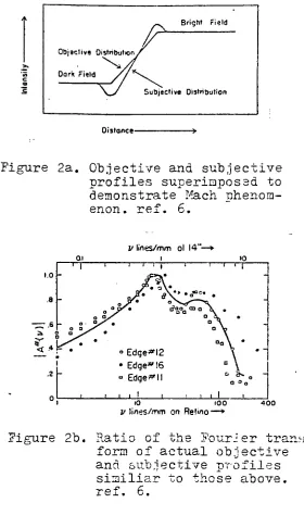
Dark Field Bright Field Subjective Distribution

Distance-Figure 2a. Objective and subjective profiles superimposed to demonstrate Mach phenom enon, ref.

6.

vlines/mm Ol 14"?

01 i 10

1.0

-1 ₁ ' ' ' ' _I

JT'A

1 1 1 I

I

a

-ojr* _o o"='

.

o O^X a _\

6 O

-Q^r m 0 \

o a o V

*

S a^* "

.1/^ \

*

<4r 0_Edge*l2 \ * ~

Edge*₁₆ a

\

.2

'

- _Edge*!!

i i r 1 t

** -i . , , 1

10 100

V lines/mm on Retina *

400

Figure 2b. Ratio of the Fourier trans form of actual objective and subjective profiles

[image:11.538.125.405.51.537.2]

quencies.

This

rather peculiar occurrence is a direct re

sult of the phenomenon of Mach Bands.

Mach

bands,

so named after Ernst Mach who first dis

covered them over one hundred years _ago, are a result of

the neural _processing sub-system mentioned before. Mach

Bands are the perception of the minimum

density

area at

an edge _{appearing lighter} than its equal

density

_surround,

and the maximum area

density

at the edge _appearing darker

than its equal

density

surround. These bright and dark

bands produce the sensation of enhanced contrast. A

typ

ical edge _profile, superimoosed with the profile of the

perceived edge is in. figure 2a on the previous page.

Lowry

and Depalma showed that

by transforming

each

profile into the spatial

frequency

domain and

taking

the

ratio of the _subjective, or _perceived, profile transform

with the objective profile

transform,

the result is a

curve with the characteristic low spatial

frequency

dip,

figure 2b.

The physiological explanation behind the phenomenon

of Mach Bands has to do with the interactions of adjacent

elements in the matrix of visual receptors.

Any

single

receptor, when excited

by

light,

has been found to send

de-receptor is proportional to the total excitation of the

surrounding receptors. For the

imaging

of an edge

by

the

eye, low excitation receptors lie adjacent to high ex

citation receptors. At the low level there is increased inhibition due to the adjacent high excitation level.

But,

the receptors that receive high excitation and lie adja

cent to the low excitation receptors receive less inhi bition than the other high excitation receptors. The re

sult is enhancement of the perceived signal

difference,

or

contrast.

Much work was done in the sixties

investigating

the

relatively new concept of spatial

frequency

response as a method of

describing

the performance of the human vis

system.

Among

_{the many} parameters which were

inves-3 tigated was sine-wave vs. square-wave response

, average

2 4-57 47 7

field luminance

*^*^''9

_viewing distance '

, viewing time , 2

and monochromatic field response .

Although Bryngdahl's work investigated the response

in the mesopic _region, the region which is of interest in

this experiment, he employed a technique of contrast match

ing

similiar to the one described earlier. His results

were dependent not _only on average field

luminance,

but on

the object contrast as well. The behavior of the curves

ex-less erratic results. Bryngdahl's contrast ratio vs. spa

tial

frequency

curves are shown in figure 3.

Since it is red light that is of interest in this ex-2

periment, Van Nes and Bouman's work, which investigated

the spatial

frequency

response at

450,

525

and 650 nm, was

consulted. In their _work, a 2 mm artificial pupil was used and the response of _only one eye recorded.

They,

however,

did use the threshold contrast method and their results are

less erratic than those of Bryngdahl. It was from Van Nes and Bouman's work that the spatial frequencies to be tested and the expected range of modulations _necessary were pre

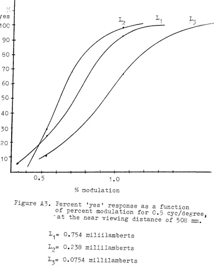
dicted. Their results appear in the appendix,figure A3. The project presented here

is,

in a _sense, a combi

nation of Bryngdahl's work in the mesopic region and Van Nes and Bouman's work with _color, conducted in a real life

environment. The viewers used both eyes to respond to the

targets,

without artificial _pupils, and in an attempt to

simulate safelight _conditions, broad band rather than mo

nochromatic light was used. Threshold contrasts _apply to the real life environment as _well, since in most cases film

defects differ minimally from the surround.

perform-anoe in the mesopic region. The

following

sections describe

the approach taken in _gathering the _necessary data.

0.005 0.01 o.os o.i as

spatiJ _{fre^u.ney (5re9/mif} of_arc)

pigure 3. Bryngdahl's results in the mesopic

region _showing erratic dependence

on object contrast. Each curve re

presents a different object con

METHODS AND PROCEDURES

It was desired to have a method of _obtaining thresh

old modulation as a _function of spatial

frequency

for the

human visual system.

Thus,

it was _necessary that modula

tion be controlled

by

this method without _{significantly}

changing the average screen luminance. The screen

lumin-is an _{important parameter} upon which spatial

frequency

re

sponse is dependent. >^'^>'

^i/hile,

in this _experiment,

data was gathered at three different screen

luminances,

the average luminace at _-any given level changed _minimally

during

testing.

For this _experiment, two slide projectors were used to

obtain _this result. The first projector contained

35

mm

slides of bar

targets,

while the second projector con

tained _only a blank field. Projected _{coincidently,} the in

tensity

of one or both of the projectors could be controlled

to vary the modulation of the projected bar target.

Since modulation was dependent on the intensities of

the two

beams,

varying these beams in increments - _as

with

neutral

density

filters - _meant that _{modulation would}

vary

in increments as well. While tne consequences of this in

terms of the judges ' responses are discussed in a later sec

Projection System

Mathematically

modeling the projection system required

that certain regions of operation be defined. These regions

are based on the _relationship of the average luminances of

each projector. Projector one contained the targets and

its average luminance L is defined below.

o

L =

*(L

+ L .

)

(i)

o ' v

max mm

where: L = maximum luminance at the screen from the target projector alone.

L . = minimum luminance at the screen

m:Ln

from the target projector alone.

Projector two provided _only a _veiling glare and its

average luminance is _simply V . Note that while each pro-si

jector has an average luminance which _{may be} varied

by

filtration,

there is a final average screen luminance

Lg

which is the sum of both of the projectors' average lum

inances.

L = V ₊ L

(ii)

s _g o

It is the value of L which must _vary minimally as

filtration is added to the system.

In _general, modulation for a two beam system such as

this one is driven

below.

L - L

.

. max mm / . . . \

M=

(m)

s L

n + L . + 2V

max mm _g

where: M = the modulation at the screen.

L n and L .

= the _{maximum and} minimum

lum-max mm . , . , ~

mances at the screen from

the target projector alone.

V = the _veiling glare luminance from

pro-jector two alone.

The three regions of operation of this system

-when

the _veiling glare equals the average luminance of the tar

get

beam,

when it is less than the average luminance of the

target

beam,

and when it is greater than the average lumin

ance of the target beam

-will each have different rela

tionships between screen modulation M and filter

trans-mittance t.

Region One

In this region the veiling glare is set equal to the

average luminance of the target projector. The screen's

average luminance that we want to maintain is _exactly that

L = L

(iv)

so

Thus,

attenuating

the target beam with a filter of

transmittance

t,

will necessitate the addition of a veil

ing

glare at the screen equal to

(l-t)L

such that the

following

is true.

tIQ

+

(l-t)LQ

=

Lo

(v)

By

setting the open gate _veiling glare

initially

so that it is equal to the average luminance of projector _one,

a _{compensating relationship} will exist _wnereby neutral den

sity addee at projector one will require neutral

density

to be removed from projector two. The expression for mod

ulation

becomes,

t(L - L .

)

M =

max

Ei_

(vi)

s

t(l_v + L .

)

+ 2(l-t)i(L + L .

)

max

mm' v '

max mm'

t(L - L .

)

M = -SSS

SiaT

(vii)

s

(t

+ 1 - t)(L + L .

)

v ' v

max

' mm'

M = t(M.

)

(viii)

s 1

where: M = the modulation at the screen. s

"

t = the transmittance of the

filtration

Mi= _{the initial target modulation.}

Since

neutral

density

_filters were to be used for at

tenuation,

there was a limitation imposed on the demodula tion capabilities of the system. The least amount of at

tenuation

available is a N.D. 0.1 whose transmittance is

approximately

80%. V/ith a transmittance of

80%

on the veil

ing

glare _projector, a _{transmittance} of 20% is required on

the target projector. This arrangement provides the lower

limit of demodulation

(.20

M.

)

without _violating the re

quirement that the screen luminance remain a constant.

The second region of operation of this _system, when

the _veiling glare is less than the average luminance from

the target _projector, will be shown to have similiar limi

tations.

Region Two

When the _veiling glare is made less than the average luminance of the target

beam,

it is _supplying the smaller

percentage of the total screen luminance.

Thus,

_any changes made at the _veiling glare projector will not _{significantly} affect average luminance at the screen. Since we are striv

ing

for minimal changes in average screen

luminance,

_{it ap}

at the _veiling glare projector to control _modulation, while

leaving

the target beam unfiltered. This system allows av

erage luminance to vary,

but,

if _controlled, the lumin

ance will _vary over _only a small range.

Suppose the _veiling glare is some fraction R of the

average luminance L . The average screen luminance L _, in

this case, will equal

(R

+ 1

)L

. The effect on modulation

as neutral

density

is introduced to projector two is shown

below.

M =

^x

jEiS

(ix)

s

L + L . + 2tR(L + L .

)

max mm max mm'

M =

!

M.

(x)

3

1 + tR 1

where: M = the modulation at the screen. s

t= the transmittance of filtration at pro

jector two.

R= the ratio of the _veiling glare V to

average luminance of projector one L _,

and is always less than 1.0.

M.= the initial target modulation.

In this case, if R is kept very small, the average

luminance will _{vary minimally} as the attenuation is added

to the system, but the minimum modulation attainable be

limit to the modulations possible. The _remaining region of

operation,

however,

allows unlimited demodulation below a

certain

level.

Region Three

This third region of _operation, where _veiling glare

is greater than the average luminance of the target

beam,

was the one chosen for this experiment. As will be _shown,

its chief advantage is in its _ability to obtain _very low

modulation levels such as were needed for this experiment.

As in the previous region of _operation, filtration oc

curs where it will have the least effect on the average

screen

luminance.

In this case, that is the target pro

jector.

By

_setting the _veiling glare to be some factor R

times greater than the average luminance of projector _one,

the average screen luminance becomes

(R

+ 1

)L

and the

o

modulation is affected as follows.

t(L - L .

)

M- -322

^

(xi)

S

^Lmax

+

W

+

2R*(Imax

+

W

M = M.

(xii)

s

t + R x

where: M = the modulation at the screen.

tss the transmittance of the filtration

at projector one.

R= the ratio of _veiling glare V to the

average luminance of projector one L ,

and is always greater than 1.0.

M.= _{the initial target modulation.}

With this _system, as R

increases,

the average screen

luminance will remain within tighter limits when the at

tenuation at projector one is varied. The maximum modula

tion level _attainable,

though,

decreases. It is possible

to reach _extremely low modulation levels regardless of

the value of R

by

_simply

increasing

the attenuation at pro

jector one.

It should be noted that the above expression for mod

ulation

(equation

(xii))

is a general one that would _ap

ply to any two projector system where the _veiling glare _is

kept constant. The stipulation that R must greater than 1.0

is stated so that the average screen luminance will _vary

minimally.

In order to point out the characteristics of each

system, table 1 shows how modulation varies with trans

mittance for the three systems. The value of R is

0.5

for

system two and 2.0 for system three.

Characteristic of system one is a broad range of modu

N.D. t Region 1 Region 2 Region

3

0.0 1.00 M.

l

0.67Mi

0.33M

0.1

0.79

0.79M.

0.71Mi

0.29Mi

0.2

0.63

0.63M. 0.76M.

0.24M

0.3

0.50 0.50M.

l

0.80M. l

0.20M.

0.5

0.32

0.32Mi

0.86M. 0.1

3M

0.7

0.20

0.20Mi

0.911^

0.092^

1.0 0.10

0.95Mi

0.05Mi

1.5

0.03

0.99M

0.011^

2.0 0.01 0.99M.

0.005Mi

Table 1. Screen modulation in terms of the in itial target modulation for the three

regions of operation as neutral den

Inherent in this system is a constant average luminance.

The other two systems allow a small range of _variability

in average

luminance.

_{System three} can decrease the tar

get modulation

by

the greatest _amount, there

being

essen

tially

no limit to the minimum modulation on the screen.

This system is best used when fine increments of low mod

ulation are desired. For these reasons and the added con

venience of _controlling neutral

density

at just one pro

jector,

this third region of operation was used for this

experiment. The next section discusses details in the test

ing

of this model.

Verification of the System

In order to test the _system, the maximum and mini

mum luminances of each target were measured _using a

\

de

gree Spectra Spot Meter. From this

information,

both the

initial modulation and average luminance of each target

could be determined. These readings were made

directly

from the target projections onto the rear projection

screen that was used in the experiment with the magnifi

cation and _geometry the same as would be presented to the

judges. The average luminance and initial modulation of

each target is listed in the _appendix, table A1 .

order to obtain the

extremely

low threshold modulations

necessary

in this experiment. The value of

R,

the ratio of

the _veiling glare to the average luminance of the

target,

was on the order of

2.0,

but varied

depending

on the aver

age

luminance

of each target. The screen modulation for

each target is tabulated as afunction of filtration in ta

ble A2 of _{the appendix.}

To determine if the model was _adequately

describing

the demodulation due to

filtration,

the maximum and min

imum luminances were read for various ajuounts of filtration

and the modulations calculated. These modulation levels

verified the predictions made from using equation

(xii).

To get an idea of how much variation in average screen

luminance could be expected _using this _system, the two

extreme cases are taken. When the transmittance of filtra

tion at the target projector approaches _zero, the average

screen luminance approaches 2L . When the

transmittance,

on the other

hand,

approaches _one, the average screen lu

minance approaches 3L .

Thus,

the average luminance can

change, in the worst _case,

by

a factor of

0,667

or _ap

proximately

i

stop.

Target

Making

p

fre-quency response of the visual system under similiar con

ditions was consulted in order to determine the

appropri-aterange of spatial frequecies to be tested.

0.5

- 9.0

cycles/degree were _desired since this included the low

frequency

region which was expected to be _non-linear,

as well as higher

frequencies

in a region where the curve

was expected to become linear.

Thus,

it was hoped that suf

ficient information would be obtained to determine the di

rection that the curve would take in the higher frequencies.

Since high

frequency

targets are difficult to _make, five

lower

fequency

targets were made and the _veiwing distance

of the judges increased

by

a factor of

3

to increase the

angular frequency.

Targets _{corresponding} to

0.5,

1.0,

1*5.

2.0,

and 3.0

cycles/degree were desired at the chosen _viewing distance

of 508 mm

(20

in). Table

A3

in the appendix expresses

the angular frequencies

(cycles/degree;

in terms of ab

solute spatial

frequency

in cycles/mm.

In order to make the

targets,

the magnification of

the projection system had to be taken into account.

Using

a Kodak Carousel 600 Projector with an

f/3.5

zoom

lens,

102-152 _mm, the minimum magnification at the rear projec

tion screen was 5.45x. The required spatial frequencies

of the targets with the magnification taken into consider

At the _{far viewing}

distance,

_{tha angular subtense of}

each target would be 3x

less,

thus the spatial frequencies

of the same targets would be

1=5,

3.0,

4.5,

6.0,

and 9.0

cycles/degree. There is an _overlap in the spatial frequen

cies tested at each distance in order to determine a cor

relation between the two sets of results.

A high contrast contact print of a 4 cycle/mm chrome

on glass Ronchi

Ruling

was used in the enlarger to make

these

targets.

The _necessary enlargements were made onto

35

mm

Panatomic-X

film.

Since _very low contrast level were _going to be neces

sary

during

the _experiment, target modulations were made to

approximately 20%

rather than a _higher value which would

only require more demodulation upon projection.

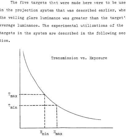
Low contrasts were obtained

by

first _gray

flashing

each _strip of film and then _proceeding with the target

exposure. Based upon the characteristic curve of the

film,

expressed in terms of transmission vs. _exposure, the ne

cessary gray flash exposure and bar target exposure could

be calculated. Figure

4,

on the next _page, shows the char

acteristic curve and the desired maximum and minimum

trans-mittances to yield a contrast of 20%. Notice that the _gray

flash exposure determines the minimum

density

on the

film,

while the target exposure is an additional increment which

The five targets that were made here were to be used

in the projection system that was described earlier, where

the _veiling glare luminance was greater than the target's

average

luminance.

_The experimental utilizations of the

targets in the system are described in the

following

sec

tion.

Transmission vs. Exposure

T

max

T

'mm

E . E mm max

Figure 4. Transmission vs. exposure

indicating

maximum and minimum transmission required to

give a modulation of 20% and their _{corresponding}

exposures. Emin= gray flash exposure.

E - E

. = bar target exposure.

[image:29.538.56.465.77.522.2]

EXPERIMENTAL

In this

experiment,

it was desired to simulate the

conditions of film inspection in order to determine the

threshold contrasts of the human visual system in this

environment.

Thus,

binocular _viewing of low contrast pro

jected bar targets on a red low luminance field v/as to oc

cur. Two different _viewing distances were chosen to in

crease the range of spatial frequencies in cycles/degree

that would be tested.

Judges

There were 8-10 judges at each luminance level tested

whom were asked to respond to the projected targets. For

the near _veiwing

distance,

each judge was asked to rest

his head against a padded post set in front of the screen

so that the average observer's eye would be 508 mm from the

veiwing screen. When the veiwing distance was to be in

creased, the judges were asked to lean their head back

a-gainst the corner made

by

the door and door jamb in the

rear of the laboratory. In the average _observer, this put

their eyes _{approximately} 1524 mm or

5

ft. from the pro

Each judge was given a dark adaption period of 20

min-utes based on Cornsweet's data. When the veiwer's eyes

were

fully

_{dark adapted, the tv.ro} slide _projectors, well

-baffled,

were turned on and the veiwer was presented with

an elliptical field on a dark surround. The horizontal

width of the ellipse was 148 _mm, while the height was 107

mm. The elliptical

target,

with its rounded edges reduces

the perceived contrast enhancement _alonga

boundary,

while

allowing

the greatest number of cycles to be present with

in the

field.

The

testing

began with _presenting a blank slide to

the judge so as not to mistake the various irregularities

across the field for a target. Data collection was then

started as the five targets were presented at various modu

lation levels to the judge. As mentioned _previously, neu

tral

density

filters were used to _vary the screen modula

tion. Since this was a _{non-analog system, only} certain mod

ulation levels were allowable on the screen.

Thus,

the

judges had no control over what modulations were presented

to them. This method of forced choice required that the

judges respond either 'yes' or 'no' to the perception of

contrast on the screen.

The total

testing time,

including

dark

adaptation,

was

aproximately one hour per judge. To reduce the total ex

over-lapped so that the second judge dark adapted

(or

'field'

adapted)

during

the last 20 minutes of the first

judge,

and so on.

Target Slides

There were six slides to which the judges were to re

spond, five of which were the target slides. The sixth

slide was a blank with an average transmittance similiar

to the other

five.,

which was entered into the _group to

determine the _ability of a judge to discern a blank field

in the midst of the low contrast targets.

Furthermore,

blank slides separated each of the target slides. The ad

vantage to this was in _allowing the judge to adapt to a

blank field between

targets,

negating the possibility of

an erroneous response due to an after image effect. The

blank fields between targets were _used, in _addition, to

change the filtration at the target

projector-^hese target slides were arranged in a carousel and

their order undisturbed throughout the entire experiment.

The experimental set _up and apparatus are described in the

Apparatus

Recall that a _tv/o projector _{system, consisting} of a

veiling glare projector and a target _projector, was chosen

for this experiment so that modulation of the targets could

be varied while average luminance remained _nearly constant.

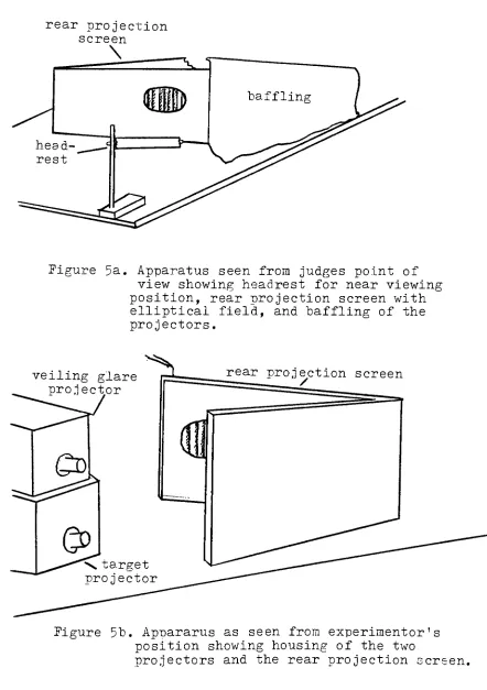
This system is shown in figure 5a and 5b on the next page.

The _veiling glare projector and the target projector were

covered with black boxes and placed one on

top

of the oth

er. The coincident beams appeared on the rear projection

screen through an elliptical window which defined the

field. The surround was _completely opaque in ordej? to re

duce _stray reflections and glare.

The rear projection screen,- a 18 in.

by

24 in. _screen,

had a folded optical axis such that the projectors were

aimed at a rear mylar surface and the beams reflected on

to the latex screen.

The _projectors, Kodak Carousel 600

's,

were well baf

fled so that

they

were _completely blocked from the field

of view of the judges and so that no _stray light would

fall on the projection screen to reduce the screen modula

tion.

The neutral

density

filters to be used in this ex

periment were placed in cardboerd mounts so that

they

could

rear _projection

screen

\

Figure 5a. Apparatus seen from judges point of

view _showing headrest for near _viewing

position, rear projection screen with elliptical

field,

and

baffling

of the

projectors.

veiling

glare projector

projection screen

;arget

projector

Figure 5b. Appararus as seen from experimentor' s

position _showing

housing

of the two [image:34.538.42.484.69.696.2]

The filters were used to control the modulation on the

screen.

Modulation Control

Five different modulation levels were chosen for each

target based upon a range it was hoped would include

threshold.

Although t he order of presentation of the target

slides remained _constant, the order of the different mod

ulation levels was _randomly generated.

Modulation levels were changed

by

_adding or

taking

away neutral

density

filters from the target projector.

Filtration changes always occurred

during

projection of a

blank slide inserted between each of the target slides.

After the judge had responded to all of the slides in

the _carousel, each at a different modulation

level,

the

tray

was reset to the first slide and the

testing

continued.

After all of the modulation levels for'each of the slides

had been _presented, the entire procedure was _repeated,

giving two replicates of each per judge. The judge was

then asked to move to the _{far viewing distance} and a

howneu-tral

density

filters affected the screen modulation for

each

target.

With P-10 judges at each luminance level that

was tested and 2 replicates per

judge,

a total of 16-20

data points for each modulation were gathered for each tar

get.

Luminance

and Color

Three different low luminance

levels,

all within the

mesopic region of visual _response, were tested:

0.754,

0.238,

and

0.0754

millilamberts. The mesopic region cov

ers a range from 10 down to 10"2 millilamberts.8

As be

fore,

luminances were measured with a

i

degree Spectra

Spot

Meter.

These low luminance levels were obtained

by filtering

both projectors with the same neutral density. Included in

the filtration of each projector was a Wratten 25 used to

simulate the red safelight conditions. Its spectral trans

ANALYSIS OF DATA

This experiment was designed to simulate the low lum

inance red safelight conditions of film inspection _areas,

so that the limitations of the human visual system in this

environment could be determined. A series of bar targets

were made _which, upon _projection, v/ere viewed

by

judges.

Using

a two projector system and neutral

density filters,

the contrasts of the bar targets were varied in increments

while _{minimally changing} the average screen luminance.

The technique of _presenting to the judges modulation levels

which varied in increments is known as the method of forced

choice.

Thus,

the judges _only response to the target was

a 'yes' or a 'no' to the perception .of contrast on

the"

screen. In order to increase the range of spatial frequen

cies _presented, each judge viewed the targets from two

different _viewing distances. Three different average

lum-inace levels within the region of mesopic response were

tested under these _conditions, with 8-10 judges at each le

vel. The analysis of the response data that was gathered

is given below.

The 'yes' and 'no' responses to the perception of con

trast were tallied for each of the targets different mod

100%

'yes'

response down to 0C' 'yes'

response

depending

on

the amount of demodulation due to neutral

density

entered

into the system. The tallied data is presented in the _ap

pendix,

tables A5-A10.

For each

target,

the percent 'yes' response was plot

ted as a function of _{modulation. From} these _curves, the

threshold _contrast, or

50%

_point, could be extrapolated. :

These nine _graphs, one for each spatial

frequency

which

yielded a

50%

response _point,are in the _appendix, figures

A3-A11. Note that the highest

frequency

target at the far

viewing distance was observed even at its highest modula

tion less than 50p'

of the time therefore is not included in

the results.

Immeadiately

apparent from both the tallied data and

the response curves is

that,

_{in many cases,} there are _only

2 or

3

points between 1C0% and

G%

response. Since it is

this range which determines the shape of the _curve, it

would have been far more desirable to have more data with

in this range.

Unfortunately,

before

testing

it was un

known what range of modulations would prove to be critical.

With finer

tuning

of the _modulations, the response curves

could have been made with more confidence.

There

is,

however,

a limit to the shape that the pre

sent curves can take.

Manipulating

the curve shape when

there

is,

in the worst _case, just one point between

0%

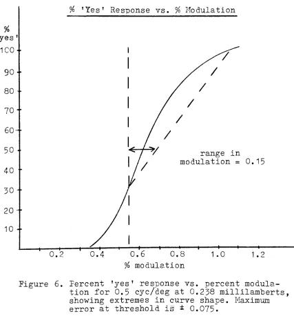
and

take. In figure 6 on the next _page, the response curve for

the

0.5

cycles/degree target at the middle luminance le

vel _{is reproduced.}

Here,

_the

only known point between 100%

and

0%

is a

30%

response at a modulation of 0,54%. The ex

tremes that the curve can

take,

a vertical line through

the 30% point and a line _connecting the

30%

to the 100%

point, mark the extreme range that the 50% point can take.

Going

from a minimum modulation of

0.54%

to a maximum modu

lation of

0.69%

corresponding to these extremes, gives a

maximum error of

0.075%.

_These

extremes _are,

indeed,

un

realistic since some assumptions can be made about the ex

pected distribution around the threshold value. A normal

distribution might be _expected, thus the response curve

would take on the characteristic S-shape and the actual er

ror in the 50% point would be less. As is obvious from the

response curves in the appendix, a.- normal distribution was

assumed.

To check this _assumption, the few distributions which

did contain greater than 2 points between the

0%

and 100%

response were plotted on normal _probability paper. These

appear in the _appendix, figure A12-A18. Recall that a

straight line through the points on normal _probability pa

per indicates that the distribution is normal. Upon visual

inspection,

all of the plots seem to tend toward a straight

%

'yes'

1C0-

90--

80--70"

60--50

40

-

30-

20--10

--%

'Yes'

Response vs.

%

Modulation

0.2

i

/

range in

modulation =

0.15

0.6 0.8

%

modulation

1.2

Figure

6.

Percent 'yes'

response vs. percent modula

tion for

0.5

cyc/deg at 0.238 _{millilamberts,} [image:40.538.57.484.186.644.2]

points were transferred to linear graph paper and a linsar

regression run. mhe narrow dispersion of points about the

line of best fit _along with the high correlation coeffi

cient indicate that the distributions in question _can, in

deed,

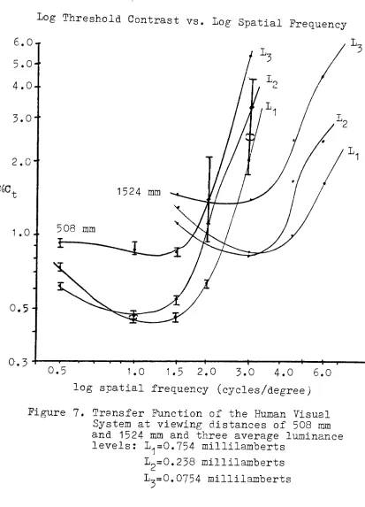
be considered normal.

The threshold contrasts _{corresponding} to the 50% re

sponse points were slotted as a function of spatial fre

quency. These _curves, the transfer functions of the hu

man visual system under red safelight _conditions, appear

on the next _page, figure 7. The two families of curves

corresponding to the two viewing distances contain three

curves _each, which correspond to the three luminance levels

at which data, was taken. The characteristic low

frequency

increase in threshold is evident, with an overall increase

in threshold contrast as the luminance level falls off.

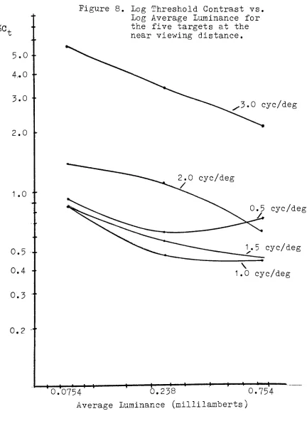
The relationship between average luminance and thresh

old modulation for the

5

targets at the near _viewing dis

tance is made clearer

by

the graph in figure 8. Here the relationship is plotted and it can be seen that there is

an overall decrease in threshold as average luminance is

increased. The lower

frequency

targets

(except

for

C.5

cy

cles/degree, whose behavior is discussed

later)

show a ten

dency

toward _reaching a minimum threshold and

leveling

off as average luminance is increased. The higher

frequency

re

log

Threshold Contrast

vs.

Log

Spatial

Freq

uency

6.0-r

5.0--4.0-.

3.0

2.0'

%C,

1.0-.

0.5-0.3

i i i

1.0

0.5

1.0 1.5 2.0 3.0 4.0 6.0

log

spatial

frequency

(cycles/degree)

Figure

7.

Transfer

Function of the Human Visual

System at _{viewing distances} of 508 mm

and

1524

mm and three average luminance levels:

1^=0.754

millilamberts

L2=0.238 millilamberts

[image:42.538.57.470.106.679.2]

5.0--4.0

-Figure 8.

Log

Threshold Contrast vs.

Log

Average Luminance for

the five targets at the

near _viewing distance.

3.0

y3.0 cyc/deg

2.0

1.0 "

0.5

0.4

cyc/deg

cyc/deg

1.0 _cyc/deg

0.3

"

0.2

--> _ i

*- t

t-0.'0754

0.238

0.754

[image:43.538.56.488.113.719.2]

o

by

Rose-" that the threshold contrast would fall off as the

inverse of the square root of the scene luminance.

Variability

Between Judges

The error bars at each data point on the curves are

based on an estimate of _{variability among} the judges at

the threshold

level.

Since _only two replicates at each mod

ulation level were presented to each

judge,

individual

re-spnse curves would be meaningless since the _only allowed

percent responses are

100?'),

50%,

and 0%.

Thus,

the var

iability

among judges at threshold cannot be found

by

de

termining

the threshold contrasts of each judge.

An alternative method of _obtaining the _variability

among judges at threhold utilizes the _variability at

100%

and at

0%

response.

Finding

the minimum modulation where

each judge saw the target

100%

of the

time,

gives a dis

tribution of responses at the 100% point.

Similiarly,

a

distribution around the maximum 0% _point, or _100% 'no' re

sponse point,. can be determined.

Taking

the variances of

each of these distributions and _averaging them will give

an estimate of the variability at the

50%

threshold point.

This data is tabulated in the _appendix, tables A 1 1-A1 6.

Placed on the transfer function curves in figure

7

are one

In _refering to figure

7,

notice that the _variability

among

judges is greatest in the hirher

frequency

regions

and there is considerable _overlap in the error bars among

the different luminance levels. In the lower

frequencies,

distributions

are narrower around each point and there is

no _overlap except at points where the high luminance curve

and the middle luminance curve cross over. This unexpect

ed phenomenon appears to be due to an artifact in the sys

tem.

System Artifacts

A possible explanation for the fact that threshold

contrasts were _unexpectedly higher under brighter viewing

conditions is the presence of a. hot soot in the _veiwing

screen. This hot _spot, which appeared in the center of the

field,

caused modulation at the edges to be _slightly greater

than at the center.

Thus,

as threshold contrasts were _ap

proached, the perception of modulation at the center was

lost at the center before it was at the edges. The size

of the hotspot in the field was dependent on the lumin

ance

level,

thus at the brightest level the hot spot was at

its largest and _conceivably took _up so much of _{the ellip}

tical field that _only the ends of the ellipse were unaf

cause _any severe problems since the narrow bars and spaces

could be seen within .the end regions. At the lov/est fre

quency,

however,

it is possible that the width of a bar

or space was as great as or -greater than the end regions of

the elliptical

field.

Thus,

as the contrast

decreased,

_only

a uniform field would perceived. If this was indeed

hap

pening, the unexpected crossover of the high and middle lum

inance _curves, which occurred at _{both viewing}

distances,

would make sense. In future work, it would be

highly

ad

visable to use a projection screen which had a more un

iform field than the rear projection screen used for this

experiment.

Another unexpected _phenomenon, which can be explained

by

the _system, is the apparent shift of the three curves

when _viewing distance was increased. Recall that the

viewing distance was tripled to obtain higher spatial fre

quency targets. It was expected that the threshold levels

from this data would _simply add more points to the near

distance _curves, extending them into the higher

freqency

region.

However,

it is obvious that an _entirely new set

of curves were generated with characteristics _very

simi-liar to the _{corresponding} near _curves, see figure 7.

For _{example, the} crossover of the high luminance and middle

luminance curves occurs at both viewing distances.

Also,

to level off in each case.

The degree of shift varies somewhat for each luminance

level,

ranging in the horizontal direction from a factor

of

3

for the high

luminances

down to approximate! 2 for the

low. The vertical shift is more consistent _among luminance

levels,

ranging from a factor of

1.75

down to 1.65. These

shifts v/ere based on the minimum thresh olds at each dis

tance. Although the shift in these three curves was unex

pected, similiar results have _subsequently been found in

the

literature.

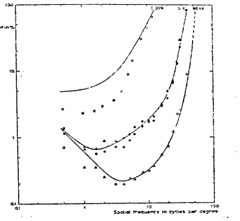
Schrober and Hilz in

1965,

measured threshold con

trasts of the human visual system and varied the _viewing

distance as a parameter. Their _results, shown on the next

page, figure

9,

indicate a horizontal and vertical shift

in the same direction as shown here. There is no correla

tion,

in _comparing their results with the ones

here,

be

tween the degree of shift and the increase in _viewing dis

tance.

3

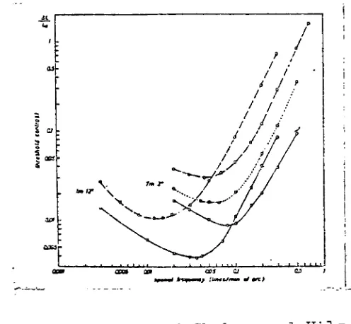
Interestingly,

Lowry

and DePalma also varied view

ing

distance in their work with the visual _system, but no

significant shift in the curves due to _viewing distance

is indicated. Their curves appear in figure 10. The es

sential difference in experimental

technique,

is that

Lory

and Depalma chose to

keep

the visual angle of the

Figure 9. Results of Shober and Hilz show

ing

the vertical and horizontal

shift of the curves as viewing

distance and visual angle in

crease from 1 meter and

12

to

7

meters and 2 . ref. 4.

CONTRAST SerOtTMT ft _/ SOUSS-MVE TEST CftjECT

C^wio*'*rt*vwr* 20 fM_

**1 I

* SpaMfr**ey (Lm/rr-manm retr^j)

Figure 10.

Lowry

and De^alma's curves do not

shift as a function of viewing dis

tance as above since visual angle

[image:48.538.105.421.77.668.2] [image:48.538.126.374.93.322.2]

Schrober and Hilz and myself chose to

keep

the field size

a

constant^

as

viewing

_distance was increased. In our _cases,

the angular subtence of the field _changed, thus targets of

the same angular

frequency

(cycles/degree)

would contain a

different number of cycles at each of the _viewing distances,

For this

experiment,

visual angle of the subtended field

decreased from 8.3

x 6.0 to 2.8

x

2.0

when _viewing dis

tance was

increased.

Savoy

and McCann show that there

is,

indeed,

a de

pendence on the number of cycles present in the field.

They

show that the shift in the transfer curves due to a

change in _viewing distance or visual angle can be described

in terms of the number of cycles in the field. Although

they

go as far as to suggest that the low

frequency

fall

off in _sensitivity is due to a decrease in the number of

cycles _present, suffice it to _say here that the number of

cycles affects the position of the curves with no apparent

change in the shape of the curves.

This leads to the question of how to define an ab

solute transfer function which can be obtained under _any

conditions, as

long

as all

influencing

factors can be

taken into account.

Thus,

knowledge of what variations

in curve position and shape that will-, occur as a function

of each

influencing

parameter would be necessary.From Sa

voy and McCann '

para-meter can be accounted for. With the _many parameters that

influence

the visual system's _performance, there is much

room for future work.

Summary

of Results

The transfer function of the human visual system

was determined for a range of low luminance red safelight

conditions. It was found

that,

in _general, there was a fall

off in contrast

sensitivity

as average luminance within

the mesopic region

decreased,

with the absolute peak re

gion of the curves

being

dependent on the _viewing distance

and,

thus,

on the number of cycles in the field.

From the results

here,

the near _viewing distance peak

occured around 1.0 cycles/degree with a small variation

depending

on field luminance. For the far viewing

distance,

the peak occurred at _{approximately} 3.0 cycles/degree.

The near _viewing distance results agree _closely with

Van Nes and Bouman's results with a similiar visual an

gle.

Van.

Nes and Bouman's results are in the _appendix,

figure A1 .

Eryngdahl's field angle is also similiar _,

however,

recall that Bryngdahl's work, also done in the mesopic

region, had erratic results

(figure

3)

due most

likely

to

the measurement technique. The contrast threshold method

re-'.!.-suits, as was

hoped,

and it is _unlikely that Bryngdahl's

results _{bear any} meaningful comparisons due to similiar

CONCLUSION

On the basis of these _results, it can be concluded

that under low luminance red safelight _conditions, thresh

old contrasts are

inversely

proportional to average lumin

ance. The exception to this is in the low spatial frequen

cies where threshold contrasts tend toward, a. constant

with

increasing

average luminance.

It was found that threshold contrasts as a function

of spatial

frequency

are dependent on _viewing distance

and,

hence,

visual angle or number of bars in the field.

Limitations of the visual system can not be determined

effectively without

having

a means of _{quantitatively} an

alyzing the effects of each of the parameters upon which

the visual system is dependent.

By filtering

out the

effects of these parameters, it may be possible to deter

mine an absolute transfer function. This type of analysis

LIST OF REFERENCES

1. T.N.

Cornsweet,

Visual

Perception,

_Academic

Press,

New

York,

1970.

2.

F.L.

Van

Nes

and M.A.

Bouman,

'Spatial Modulation

Transfer

in the Human

Eye',

JOSA

57,

p. 4-06

(1967).

3. J.J. DePalma and E.M.

Lowry,

'Sine-Wave Response of

the Visual System.

II.

Sine-Wave and Square-Wave Contrast

Sensitivity*,

_JOSA

52,

_p.328

(1962)

4. H.A.W. Schober and R. .iHilz, "Contrast

Sensitivity

of the Human Eye for Square-Wave

Gratings',

JOSA

55,

p. 1086

(1965).

5. 0.

Bryngdahl,

'Characteristics of the Visual System:

Psychophysical Measurements of the Response to Spatial

Sine-Wave Stimuli in the Mesopic

Region',

JOSA

54,

p. 1152

(1964).

6.

E.M.

Lowry

and J.J.

DePalma,

'Sine-Wave Response of

the Visual System. I. The Mach

Phenomenon',

JOSA

51,

p.740

(1961).

7. A.

Wantanabe,

T.

Mori,

S.

Nagata,

K.

Hiwatashi,

'Spatial Sine-Wave Responses of the Human Visual

System',

Vision Research

8,

p. 1245

(1968)

8. Rubin and

Walls,

Fundamentals of Visual

Science,

Charles

C. Thomas _publisher,

Springfield,

1969.

9. Kodak Filters for Scientific and Technical

Uses,

Publication No.

B-3,

Eastman Kodak

Company,

Rochester,

1973.

10. R.L.

Savoy

and J. J.

McCann,

'Visibility

of

low-spatial-frequency

sine-waves: Dependence on number of _cycles',

Saaffl* rrvui*<V eyt)*a**-

<J3'"-*-Figure A1 Van Nes and Bouman's results

for monochromatic radiation.

The values of interest for

this experiment are the

closed triangles which in

dicate data at 650 nm at

0,9

[image:55.538.109.352.125.349.2]

.hi

IX-10X-,

100"

200 300 3

?2

400 500 6G0 700 800 S00

1

j '

r

1

> '

1

1

1

! t

L

itn:

il

X-i

1

I- _!

i 1 1

~~ 1 ;

It

"

j

i TT"

i I _i 1

-X-HX _

!

! 1 1

i

1 1 ! _U_

1

1

1 ' '

, ', i

'

I i 1

I 1

1 1 i ! I t

1

1

r If"

^"H"

i i--i t _j

-| i i ; 1 1

!

!

! 1 i 1 1 ! i 1 ₁

! | '

; _{1 1}

f

'

J

;

A

^ 1

1 i - i

1

-1 ^ 1 !

1 1

1 '

If-1

N

! 1 _j

1 !

i

1

!

r i

1

' r>-^-4.

ill'

ml

200 300 4C0 SCO 600 700

WAVELENGTH(fanenwiws)

S00 SOOi

"i^ure A2. Scectrophotometric curve for

0.5

1.0

%

modulation

Figure

A3.

Percent

'yes'

response as a

function

of _{percent modulation}

for

0.5

cyc/deg

ree, at _{the near}

viewing distance

of _{508 mm.}

^.p

0.754

miliilamberts L2= _0.238

millilamberts

[image:57.538.64.482.104.642.2]

[image:58.538.55.453.133.509.2]

%

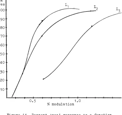
modulation

Figure A4. Percent 'yes'

response as a function

of percent modulation for 1.0 _cyc/degree,

at the near _viewing distance of 508 mm.

L1=

0.754

millilamberts

Lp= 0.238 millilamberts

0-'

%

yes

100"

90-

80--70

60-'

50--40

30

20

10

0.5

1.0 [image:59.538.59.471.139.646.2]

modulation

Figure A5.

Percent 'yes' _{response as a function} of percent modulation for

1.5

_cyc/degree,

at the near _viewing distance of 508 mm.

L.=

0.754

_{millilamberts}

L2= 0.238 millilamberts

1.5

i

% modulation

Figure

A6. Percent 'yes response as a

function

of percent modulation for 2.0

cyc/degree,

at the near _{viewing distance of 508 mm.}

Ip

0.754

millilamberts

L2= _{0.238 millilamberts}

[image:60.538.70.474.119.548.2]

3.6 4.4

%

modulation

Figure A7. Percent 'yes' response asa function

of percent modulation for 3.0 cyc/degree,

at the near viewing distance of 508 mm.

L1=

0.754

millilamberts

L9= 0.238 millilamberts

L,= _0.0754 millilamberts

[image:61.538.55.468.125.522.2]

1.0 1.8 2.6

%

modulation

3.4

Figure A8. Percent "yes'

response as a function

of percent modulation for U5 cyc/degree,

at the far viewing distance of 1524 mm.

L1= _0.754 millilamberts

L= 0.238 millilamberts

!-.= 0.0754 millilamberts

[image:62.538.53.457.122.630.2]

1.0 1.4 1.8

%

modulation [image:63.538.59.460.137.654.2]

2.2

Figure A9. Percent 'yes'

response as a function of percent modulation for 3.0 _cyc/degree,

at the far _viewing distance of 1524 mm.

L.=

0.754

_{millilamberts}

L0= _{0.238 millilamberts}

5.0

%

modulation

Figure A10. Percent 'yes'

response as a function

of percent modulation for

4.5

cyc/degree,

at the far _viewing distance of 1524 mm.

L.=

0.754

millilamberts

L= 0.238 millilamberts

[image:64.538.57.446.126.586.2]

2.6

3.4

4.2 [image:65.538.52.472.121.650.2]

%

modulation

Figure A11. Percent 'yes'

response as a function

of percent modulation for 6.0 _cyc/degree,

at the far viewing distance of 1524 mm.

L.= 0.754 millilamberts

L2= 0.238 millilamberts

98

Figure A12. Normal

probability

plot of %'yes'

response vs. modulation for

0.5

cyc/deg and near _{viewing distance.}

95

90

80

4

70

60

50

40

30

20

10

-0.754

millilamberts

0.0754

millilamberts

2

1

.2

.1

[image:66.538.51.473.98.700.2]

Figure A13. Normal _probability plot of %'yes'

response vs. modulation for 1.5

cyc/deg and near _viewing distance.

90

+

80-

70-

60-

50-

40-

30-

20-

10-5

2-1

.2

. 1

\

0.0754 millilamberts

[image:67.538.56.458.145.663.2]

90-Figure AU. Normal

probability

plot of %'yes'

response vs. modulation for 2.0

cyc/deg

and near _viewing

distance.

80-

7C-

60-50.

40-

30-

20-X

0.238 millilamberts

10

5-2

1

-

.2-.1

[image:68.538.45.475.114.671.2]

.2-. 1

-Figure

A15.

Normal

probability

_{plot of} %'yes'

response vs. modulation for 3.0

cyc/deg

and near

viewing

distance.

2

1

.5

0.238 millilamberts

[image:69.538.43.480.123.695.2]

90

Figure A16. Normal

probability

plot of %'yes'

response vs. modulation for 3.0

cyc/deg

and far

viewing

distance.

80

70

60

50

40

30

20

.754 millilamberts

10

5

2

1

.2

.1

[image:70.538.62.469.105.670.2]

93-.

95-

90-

80-

70-

60-

50-

4-0-

30-

20-

10-

5-Figure A17. Normal

probability

plot of %'yes'

response vs. modulation for

4.5

cyc/deg and far _viewing distance.

0.238 _{millilamberts}

0.0754

millilamberts

2

1

*i

m.

[image:71.538.52.470.88.714.2]

95

90-

80-70^

60-50

40-30

20

+

10

5

Figure

A18. Normal _probability plot of %'yes1

response vs. modulation for

6*1

0

cyc/deg and far _viewing distance.

llilamberts

llilamberts

2

1

.2

. 1

[image:72.538.68.455.93.664.2]

Target Target Target Target Target

12

3

4

5

*

L

o

M.

l

2.49 2.55 2.74 2.9