Network inference via adaptive optimal design

T E C H N I C A L N O T E

Open Access

Network inference via adaptive optimal design

Johannes D Stigter

and Jaap Molenaar

Abstract

Background:Current research in network reverse engineering for genetic or metabolic networks very often does not include a proper experimental and/or input design. In this paper we address this issue in more detail and suggest a method that includes an iterative design of experiments based, on the most recent data that become available. The presented approach allows a reliable reconstruction of the network and addresses an important issue, i.e., the analysis and the propagation of uncertainties as they exist in both the data and in our own knowledge. These two types of uncertainties have their immediate ramifications for the uncertainties in the parameter estimates and, hence, are taken into account from the very beginning of our experimental design.

Findings:The method is demonstrated for two small networks that include a genetic network for mRNA synthesis and degradation and an oscillatory network describing a molecular network underlying adenosine 3’-5’cyclic monophosphate (cAMP) as observed in populations of Dyctyostelium cells. In both cases a substantial reduction in parameter uncertainty was observed. Extension to larger scale networks is possible but needs a more rigorous parameter estimation algorithm that includes sparsity as a constraint in the optimization procedure.

Conclusion:We conclude that a careful experiment design very often (but not always) pays off in terms of reliability in the inferred network topology. For large scale networks a better parameter estimation algorithm is required that includes sparsity as an additional constraint. These algorithms are available in the literature and can also be used in an adaptive optimal design setting as demonstrated in this paper.

Findings

Background

Recent research in Systems Biology shows that the con-cept of ‘network’ turns out to be highly relevant at all levels of biological complexity [1,2]. In a modeling ap-proach based on networks, the components of the system under consideration are represented as nodes in a graph and the interactions as edges that connect pairs of nodes. The functioning of a network is determined by its dy-namics, i.e., the evolution in time of the nodes. The nodes usually represent the concentrations of some species and their time development is regulated via interactions with other species. At the cellular level, regulatory and meta-bolic networks are out spoken examples, but also signal-ing pathways make use of the network concept. Typical examples at the highest complexity levels are predator-prey models and ecological food webs which are in use since long. It is remarkable that not only the network concept forms a unifying element across all biological

aggregation levels, but also the mathematics needed to describe the dynamics of the network nodes show great similarities [3]. The central role of network modeling in biology implies that network inference is one of the major challenges of modern biology. The ultimate aim of net-work inference is to deduce the structure of the netnet-work as accurately as possible from data obtained in the ex-perimental practice. To obtain the necessary experimen-tal information, one usually perturbs the network in some way, hoping that the induced response is useful to be explored in some network inference approach. How-ever, if this is not done in a structured way, the harvest might be disappointing. In this paper, we consider the question how we could effectively and fast learn as much as possible of the network structure by designing the ex-perimental setup in an optimal way. It should be realized that the question we put here in a network inference con-text, is in its generality not new, since similar research is at the core of the mathematical subdiscipline called‘ sys-tems theory’, e.g., [4], and more specifically, in the subdis-cipline‘system identification’ [5]. The fascinating aspect is that insights obtained in the engineering practice may * Correspondence:[email protected]

Biometris, Wageningen University, Droevendaalsesteeg 1, 6708 PB Wageningen, The Netherlands

also be of great relevance in a life sciences setting. In an engineering context this kind of research is usually re-ferred to as ‘reverse engineering’. In this paper we also aim at connecting the still too much separated realms of scientists in biology and engineering.

Before getting into details, it is important to remark that network inference may aim at different levels of ac-curacy [6,7]. The lowest level approach leads to a rela-tively rough impression of the network structure. Given the nodes, one uses the data to find out whether a coup-ling exists between any pair of nodes. In mathematical terms, the network is represented as a graph with undir-ected edges and the inter action is not made explicit, e.g., in terms of an equation. An undirected edge indicates that the dynamics of the two connected nodes are corre-lated due to some interaction, but the character of this interaction is not pointed out in detail. For example, the first node could affect the second one, but the interaction could also be the other way around. This case is espe-cially relevant if the data contain steady state levels of the nodes obtained after perturbing the system a consider-able number of times, e.g., via a knocking out procedure in gene networks. For this case a number of statistical in-ference methods have been developed that yield undir-ected graphs as outcome [8-11]. The next level of accuracy is to strive for a directed graph, in which the edges are arrows. The direction of an arrow then indi-cates a causal relationship [12]. The most sophisticated level is to deduce more detailed information on the char-acter of the interactions. One then tries to answer ques-tions such as: Is it a promoting or an inhibiting interaction (in regulatory networks), is it a linearly in-creasing, saturating, or decaying interaction (in metabolic networks), etcetera [13,14]. In this paper we aim at the third level of accuracy by including the estimation of the strengths of interactions. A common procedure to gener-ate data is to perturb the system under consideration in a more or less random way. The change in the observed data is then analyzed to infer information about its struc-ture. In practice this may lead to very poor results, since it is not assured that the chosen perturbation is really useful for inference purposes. In this paper we propose to follow a much more advanced approach, in which the perturbations are designed such that they contain the op-timal amount of information, given the available data. This approach also starts with a more or less randomly chosen perturbation, but we show that the information from such a first step can be effectively used to design a second perturbation that yields enhanced insight in the network structure. So, we maximize in advance the infor-mation content of the second perturbation, given the insight deduced from the first perturbation. This maximization is based on improving the condition num-ber of the so-called Fischer Information Matrix of the

system. If required, this procedure could be repeated to refine the inference results further.

Our research focuses on networks whose dynamics are described in terms of ordinary differential equations (ODE). We assume that it is possible to observe the net-work while it develops in time, so that the data consists of time series of some or all of the network components. The general ideas of the present approach are widely ap-plicable and not at all restricted to a special type of net-work or level of complexity. For illustrational purposes we will make use of a gene is taken from [15]. This system has been used earlier in several studies to explain and il-lustrate the principles of other inference methods in sig-naling and gene networks [16-18] and turns out to be very useful for this purpose. Next, we apply our method to the Laub-Loomis model [19], which describes oscilla-tions in excitable cells of Dictyostelium, and show that our new procedure is very effective in reconstructing the underlying network, just by slightly perturbing system and observing its recovery to its natural oscillatory behavior.

The paper is organized as follows. In the next section we will first introduce two motivating examples in which reconstruction of a directed graph representing the interaction nodes of the network is the primary goal. Then we will further elaborate on the details of adaptive optimal input design [20] and explain the method. Finally, the methodology will be applied to the two mo-tivating examples explained earlier and some results will be presented and discussed.

Methods

Two motivating examples

In this section we introduce two biological systems that will be used later on to illustrate how our adaptive opti-mal design approach works in practice. For both models characteristic parameter values are taken from the litera-ture. These values are used to generate artificial data and to mimic real practice these data are spoiled by add-ing noise. The present aim is to show how the para-meters can be efficiently estimated from the data in an adaptive manner.

mRNA synthesis and degradation Let us consider the well-known Kholodenko case as a motivating example [15]. It consists of a small four gene network and the gene activity is reflected by the synthesis and degrad-ation of mRNA as follows:

_

x1ð Þ ¼t νsyn;1νdeg;1 ð1Þ

_

x2ð Þ ¼t νsyn;2νdeg;2 ð2Þ

_

x3ð Þ ¼t νsyn;3νdeg;3 ð3Þ

_

where x t_ð Þ stands for differentiation of x(t) with respect to time [h], and the synthesis and degradation rates are given by the following non-linear relationships:

νsyn;1¼V1s

1þA14ðx4=K14aÞn14

1þðx4=k14aÞn14

ð Þð1þðx2=k12iÞn12Þ

ð5Þ

νsyn;2¼V2s

1þA24ðx4=K24aÞn24

1þðx4=K24aÞn24

ð Þ ð6Þ

νsyn;3¼V3s

1þA32ðx2=K32aÞn32

1þðx2=K32aÞn32

ð Þð1þðx1=K31iÞn31 Þ

ð7Þ

νsyn;4¼V4s

1þA43ðx3=K43aÞn43

1þðx3=K43aÞn43

ð Þ ð8Þ

νdeg;1¼V1d

x1ð Þt

x1ð Þ þt K1d

ð9Þ

νdeg;2¼V2d

x2ð Þt

x2ð Þ þt K2d

ð10Þ

νdeg;3¼V3d

x3ð Þt

x3ð Þ þt K3d

ð11Þ

νdeg;4¼V4d

x4ð Þt x4ð Þ þt K4d

ð12Þ

The values of the parameters in these expressions are presented in Table 1.

For simplicity we start by assuming that each time an experiment starts them RNA transcription and degrad-ation rates are in equilibrium, i.e. there is a steady state for all four states in the model. This meansx_1ð Þ ¼t

_

x2ð Þ ¼t x_3ð Þ ¼t x_4ð Þ ¼t 0. Furthermore, we assume, just

as in the original paper, that we can influence the max-imum transcription rates{Vis, i=1,. . .,4}thereby silencing the synthesis of mRNA at will. In other words, the max-imum transcription rates represent an input signal that we can manipulate (or perturb) in such a way that infor-mation regarding the structure of the network is revealed through the stimulus-response data. An inter-esting (and challenging) aspect is that, in practice, it is notknown what the exact values of the input signals are. Put differently, the (constant) input stimuli (or excitation signals) are in this case a natural part of the

identification problem and these values are included in the parameter estimation problem. The ODE system in equations (1)–(12) can be written in the general form

_

x¼f xð ;θ;uÞ ð13Þ

Here, x is the state vectorx = (x1,x2,x3,x4)T, u is the vector containing the inputs, so u = (V1s,V2s,V3s,V4s)T,θ is the vector containing the remaining parameters in Table 1, and f is the vector valued function defined in equations (5)–(12).

If we linearise the above equations and evaluate the resulting equations at the steady state xss alinear state space model is obtained that reads as

dð Þδx

dt ¼Aδxð Þ þt Bδu ð14Þ

where δx(t) and δu are now the deviations from the steady statexssand the corresponding (steady) input uss that maintains this steady state. The matrix A in equa-tion (14) contains the so-called interacequa-tion coefficients of the network and these correspond to adirected graph where there is an interactionfromnodej tonodeiif the corresponding matrix element aij6¼ 0. We note that, of course, this linearisation is alocalproperty that depends on our choice of the linearisation point in state space where we derive the linear system (14). However, it is important to realize that, if nodes i and j are not con-nected, the matrixA has zeros at positionsijand ji, re-gardless of the linearisation point that is used! The question of optimal experimental design now comes down to choosing the entries of the vector δu in such a way that matrix pair [A,B] can be estimated in an opti-mal manner.

Laub-Loomis model–the no-input case A well-known example of an oscillating network in systems biology is Laub-Loomis’ model of the molecular network under-lying adenosine3’-5’-cyclic monophosphate (cAMP) as observed in populations of Dyctyostelium cells [19]. The model incorporates changes in the activities of cAMP and consists of a set of seven ordinary differential equa-tions (one for each state) that reads

_

x1ð Þ ¼t k1x7k2x1x2 ð15Þ

_

x2ð Þ ¼t k3x5k4x2 ð16Þ

_

x3ð Þ ¼t k5x7k6x2x3 ð17Þ

_

x4ð Þ ¼t k7k8x3x4 ð18Þ

_

x5ð Þ ¼t k9k10x4x5 ð19Þ

_

x6ð Þ ¼t k11x1k12x6 ð20Þ

_

x7ð Þ ¼t k13x6k14x7 ð21Þ

Table 1 Parameter values mRNA synthesis and degradation

V1s= 5 A14= 4 K14a= 1.6 K12i= 0.5 n12= 1 V1d= 200 K1d= 30

V2s= 3.5 A24= 4 K24a= 1.6 n32= 2 n14= 2 V2d= 500 K2d= 60

V3s= 3 A32= 5 K32a= 1.5 K31i= 0.7 n31= 1 V3d= 150 K3d= 10

V4s= 4 A43= 2 K43a= 0.15 K12i= 0.5 n43= 2 V4d= 500 K4d= 50

where the parameter values for the constants {ki,

i=1,. . .,14} are given in Table 2. For these parameter

values the system shows oscillating behavior.

In the first motivating example we used the maximum synthesis rates as system inputs. Here, we assume that this oscillatory system can be perturbed by kicking it out its steady limit cycle. Since this cycle is asymptotically stable, the system will converge back to it. It is just the way in which this return happens, that provides us with the additional (and necessary) information to estimate the network structure. The linearised version of the Laub-Loomis model reads

dð Þδx

dt ¼Aδxð Þt ð22Þ

If we allow a Dirac pulse, we simulate a sudden change in the state vector values so that the system is ‘kicked’ from its steady oscillation and needs to recover from this

‘shock’, returning (after some time) to its initial oscilla-tory behavior. Put differently, in mathematical terms we allow‘inputs’to be of the form bδ(t), where bis a vec-tor with dimensions equal to the state vecvec-tor x(t), so that

dð Þδx

dt ¼Aδxð Þ þt bδð Þt ð23Þ

If we assume the perturbation δu to be a Dirac delta function (or better, aδ-distribution), the question of op-timal experimental design now becomes one of finding the values of the entries in the vectorbthat yield an op-timal estimateA, i.e., an estimate  with lowest possible uncertainty bounds.

Parameter estimation–towards adaptive experimental design

For a given choice of our input perturbation, e.g., δuin our first motivating example that contains four silencing-percentages for each of them RNA synthesis processes, we now perform a simple step response ex-periment for each of the four inputs {ui (t), i=1,. . .,4} and this yields an observation record of mRNA concen-trations. In Figure 1 we see an example of such data that includes 20% error in the observed mRNA concentra-tions after a random relative perturbation (between-50% and 50%) of all input parameters {Vis, i = 1,. . .,4}in the original (non-linear) model.

Since there are four parameters{Vis, i = 1,. . .,4}, there are four ‘inputs’at our disposal that we can use as per-turbation candidates. In the following we assume that four separate perturbations of all inputs are generated with random values between−50% and 50% of the steady state input values contained in the vectorxss(that corre-sponds to the initial steady stateuss).

Schmidtet al.[16], inspired by the methods and results of [15], applied linear regression to data obtained by vir-tual experiments using the original system model as a simulation tool. Based on calculated deviations from the steady statexssa linear regression formula was obtained with the coefficients of matrices Aand Bas unknowns. Schmidt successfully computed the interaction coeffi-cients, including the unknown input perturbations, from response data. For clarity it is noted that the step-response data represents thedynamic transient behavior from one steady state to another steady state. This is different from the approach presented by Steinke and co-workers [21], where an interestingstatistical method-ology was applied with the same idea of iterative experi-mental design in mind, but for thesteady statesonly, i.e. with no dynamic transient behavior included.

It should further be noted that the regression method applied here only works for relatively small scale pro-blems in which the number of states is not too large. This is mainly because of the limitations in the applied parameter estimation method (see below for details) which easily introduces identifiability problems for large scale networks where the number of parameters to be estimated in the Jacobi matrix is simply too large. The disadvantage of ordinary least squares estimation, how-ever, can be remedied for larger scale networks by more advanced parameter estimation algorithms that include sparsity of the network as an additional constraint (see e.g. [22] for a convex linear-programming approach.) Table 2 Parameter values Laub–Loomis

k1= 2.0 k2= 0.9 k3= 2.5 k4= 1.5 k5= 0.6 k6= 0.8 k7= 1.0

k8= 1.3 k9= 0.3 k10= 0.8 k11= 0.7 k12= 4.9 k13= 23 k14= 4.5

Parameter values for the cAMP model. These values were taken from [19].

A discretized version of the linear model (14) with sampling intervalΔt=tk+1−tkreads

xðkþ1Þ ¼Φxð Þ þk Γuð Þk ð24Þ

¼ðΦ ΓÞ xð Þk uð Þk

ð25Þ

with (see e.g. [4])

Φ¼eAΔt ð26Þ

Γ¼ Z tkþ1

tk

eAðtkþ1τÞ_Buð Þτdτ ð₂₇Þ

In summary the parameter estimation method pro-ceeds as follows:

Step 1. Collect Nobservations of the state vectorx in the original non-linear model (13) with a sampling inter-val Δt. Subtract the steady state xss from these observations.

Step 2. Calculate the difference between consecutive time instances of the obtained measurements in step (1) and stack these differences in a (n× (N − 1)) matrixM with n the dimension of the state vector x and N the number of data points.

Step 3. TakeMn as the 2nduntil the last column ofM

and take Moas the 1st until the last but one column of M. Here, the subscriptsnandostand fornewandoldto denote a cause-effect relation between the matrices Mn

andMo.

Step 4. Augment the matrix Mo with a (1 × (N − 1)) row of 1’s. This is to estimate the input sequence

{Δu(k) =Γu(k),k = 0,. . .,N−1}. Denote the resulting

aug-mented matrix withMa.

Step 5. An estimate of the matrices Φ and Γ is now calculated via linear regression (see [16]) as

^

Φ Γ^

¼MnMaT MaMaT

1

ð28Þ

Step 6. Translate the discrete time result [Φ^ Γ^] back to continuous-time (see e.g. the standard textbook [23]), yielding the estimatesA^ andB^.

At this point it should be mentioned that the familiar parameter estimation method in the above does not ex-plicitly include any analysis of theuncertaintyin the par-ameter estimates obtained, although this is of course an important measure of the quality of the parameter esti-mates that have been obtained using the simple regres-sion formulae (28). Our goal in the current paper is to performmodel based experimentsthat minimize the un-certainty bounds on the parameter estimates‘on-the-fly’. To explain best what we mean with this the reader is re-ferred to Figure 2 in which the adaptive optimal input design methodology is depicted as an iterative loop. Starting with an initial random perturbation/experiment one moves on to a first parameter estimate [A^, ^B] of the Jacobi matrices [A, B] following the 6-step procedure out lined in the above. Since at this point an approxi-matemodel is available, one can progress by designing a new perturbation/experiment in such a way that a norm of the so-called Fisher Information Matrix (FIM) is opti-mized. The FIM incorporates the parametric output sen-sitivities _{dθ τ}dy_ðT^_;θÞ, where y is the output vector which, in

0 0.1 0.2 0.3 0.4 0.5 0.6 0.7 0.8 0

0.2 0.4 0.6 0.8 1 1.2 1.4

time [hr]

mRNA concentration

x1 x2 x3 x4

the two case studies discussed in this paper equals the state vector x since all states are assumed measurable with measurement error 2(k), (k=1,. . .,N), that is assumed to be sampled from a Gaussian white noise se-quence with co-variance matrix Q. We note that the parametric output sensitivity_{dθ τ}dy_ðT^_;θÞ can be calculated via the original state space model (13) (see e.g.[20]) through simple differentiation of the state equations with respect to the parameter vector θ. The FIM represents a meas-ure of the information content of the given input-output data with regard to the parameter values of the para-meters θ in the model. We choose to minimize the so-called modified E-norm of the FIM [24], which is defined as the ratio of the maximum eigenvalue of the FIM by its minimum eigenvalue, i.e.,

F tf; ^θ

¼ Z tf

0 dyT^ dθ τð ;θÞQ

1 dyT^

dθ τð ;θÞdτ ð29Þ

F tf; ^θ

Emod¼

maxf gλF

minf gλF

ð30Þ

where tf marks the duration (final time) of our experi-ment and where we have denoted with ^θ the fact that the FIM can only be calculated based upon the best knowledge we have available of the parameter values and notbased upon the true values θ*. In practice this optimization can be performed crudely by evaluating a large number, say N = 1000, of random perturbations (through simulation of the approximate model (13) with the pair [A^;B^]) and evaluate the modified E-criterium for each of these perturbations. Once the N perfor-mances have been calculated we choose the perturbation that is associated with the minimum of the N modified E-criteria. For clarity we note that optimizing the FIM with regard to some norm can be seen as away to better condition the matrix inversion in equation (28). For in-formation rich experiments the matrix Ma MaT can be shown to be better conditioned and, hence, the inversion is less prone to numerical errors that can easily result in case of a badly condition matrix.

Having thus progressed to the bottom-right circle in Figure 2, we continue to apply the‘optimal’perturbation to therealsystem, yielding an additional set of observa-tions that can now be used for a second parameter esti-mation exercise. We have now turned full circle and can start again with an improved estimate of the system [A, B], i.e. [A^1;B^1]. Several iterations of the loop in Figure 2 will now yield parameter estimates that have been inferred from an increasingly rich set of observa-tions. In other words, we have maximized the information content of the model parameters to the best of our (current) knowledge of the network as to converge rapidly to the true parameter values contained in the matrix-pair

[A,B]. Through minimization of the uncertainty bounds on the parameter estimates via optimal input design a better conditioned parameter estimation problem is gained and this is highly preferred above the ad-hoc ap-proach where random perturbations are used as an ex-perimental ‘design’. Although the above methodology (and more specifically the parameter estimates that are obtained using simple linear regression as in [16]) can only be used for relatively small networks, the adaptive input design approach can easily be extended to larger scale problems if other parameter estimation algorithms are utilized that can better handle larger scale networks (see e.g. [22] for a linear-programming approach to the parameter estimation problem for large networks). The message we would like to convey in the current paper is not about a parameter estimation algorithm, but about utilizing such an algorithm in the best possible way as to obtain reliable parameter estimates.

Results

Kholodenko case study

On the basis of a random perturbation (with maximum perturbations of 50% for all four maximum transcription rates in the original non-linear model) we obtained arti-ficial time series for all four components of x, i.e. the four mRNA concentrations, with a time-interval ΔT = 1 minute and for a length of 0.5hr, so that N = 30. We added 5% noise on these readouts. Furthermore, we assumed the matrix Bto be diagonal. This implies that the perturbationsδuinfluence the corresponding mRNA state directly. The first data sets were generated by per-forming 5 random perturbation experiments in a row and estimating the matrix A from these 5 experiments, yielding an estimate forÂthat is summarized in equation (33). The numerical values forÂ(deduced from 5 random experiments) together with their true values are:

A¼

6:45 0:00 2:31

0:00 2:92 8:17 2:80 0:00

0:00 0:00 14:46

10:22 2:54 3:93 0:00 9:74 0 B B @ 1 C C

A ð31Þ

^

A¼

7:15 0:78 1:51 1:74

2:53 8:19

1:63 1:65

1:69 0:039 8:59 0:37

3:20 5:83 0:23 8:56 0 B B @ 1 C C

A ð32Þ

original non-linear system model to create a new data set and this data set was again used to estimate Â, resulting in a second estimate of the Jacobi matrix, etc. This procedure was repeated until 5 experiments (using OID for the second to fifth experiment) were computed. The final values for the matrix entries in Âwere found to be:

^

A¼

6:50 0:68 3:05

0:91 3:14 7:66 3:91 1:45

1:36 3:20 15:18

10:25 2:43 3:15 0:26 9:54 0

B B @

1 C C

A ð33Þ

These results have also been included in Figure 3 which shows a comparison between the final estimate of the two approaches (OID and random). As to better get insight in the success rate of OID we repeated the above procedure 150 times. In Figure 4 a comparison of the two methods is presented in a graph to see the differ-ence in performance. Each point in this graph represents a pair of sum-of-squared-errors (of the parameters in the Jacobi matrix) for an optimal input design (x-coordinate) versus a random design (y-coordinate) series of 5 experiments in a row, repeated for 150 trials. The liney=xseparates the two cases and we found that for 82% of the 150 pairs (OID, Random Design), the OID results were better, i.e. the x-coordinate wassmaller than the y-coordinate. Apparently, random design can still be better than OID in 18% of the cases and this can

be understood since a wrong first estimateÂin the first OID experiment means that we design inputs based on erroneous information that points us in the wrong direc-tion for designing a better experiment. These results

cor-roborate with the fact that if we reduce the

measurement uncertainties on the sensors, OID

becomes even better than Random Design because it has a better starting point in the series of 5 experiments. More specifically, after reducing the measurement error to only 1%, the success rate of OID versus Random was 91%.

Laub-Loomis case study

The Laub-Loomis case study presents us with a far more challenging problem in comparison to the Kholondenko case study. This is mainly because in this particular case study 49 entries in the Jacobi matrix have to be esti-mated with linear regression, which is a large number. Furthermore, the non-linearity of the model introduces additional difficulties. It is therefore required to use rela-tively small perturbations in the initial condition x(0) as to not divert too far from the linearity assumption that underpins the linearized perturbation model. Since small perturbations are difficult to trace back if the noise on the data is too high, we are certainly limited in our possibilities.

To perturb the oscillatory Laub-Loomis model we apply a ‘shock’-effect to each of the entries in the state vector x(t) at time t = 0 and observe how the system

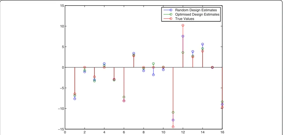
0 2 4 6 8 10 12 14 16

−15 −10 −5 0 5 10 15

Random Design Estimates Optimised Design Estimates True Values

recovers to its normal oscillatory behavior. An example of data from a random initial perturbation are presented in Figure 5. For the sampling interval of this observation record we assumedΔtto be 0.1 hr. Furthermore, the data set includes 20% artificial noise on the deviated observa-tions, i.e. the observed value xobsminus its nominal value

xnom where the nominal value refers to an unperturbed oscillatory behavior. It can be observed in Figure 5 that a recovery of the initial perturbation to a‘steady’oscillatory behavior (solid lines in figure) is present.

We found in the initial run that the estimated param-eter values are still far off from the true paramparam-eter

0 100 200 300 400 500 600

0 100 200 300 400 500 600

Sum of Squared Errors OID

Sum of Squared Errors Random Design

Figure 4Comparison plot of Random Design versus Optimal Input Design (OID).This graph shows the sum-of-squared-errors in the parameters (Jacobi matrix entries) for 150 runs of our algorithm for a series of 5 experiments. Each run is a point in this graph with coordinates (Random, OID) where Random stands for the sum-of-squared-errors for the Random run and OID stands for the sum-of-squared-errors for the OID run that started with the same initial estimate of the matrixAthat was obtained in the first random experiment.

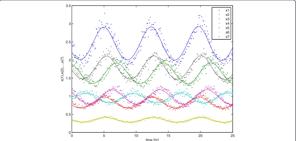
0 5 10 15 20 25

0 0.5 1 1.5 2 2.5 3 3.5

time [hr]

x(1),x(2),...,x(7)

x1 x2 x3 x4 x5 x6 x7

values. In order to find better estimates these initial esti-mates are now used for the next experimental design. Hereto the model (22) was evaluated for 250 random perturbations and for each of those 250 (virtual) experi-ments a modified E-criterion for the FIM was calculated. Taking the minimal value of these E-criteria lead to an improved perturbation that was subsequently applied to the real system (15)–(21). The second data-set was then used in a second parameter estimation exercise and OID procedure was repeated another time so that 3 experi-ments in total were used. In Figure 6 we see the final es-timation results after 1 random and 2 OID experiments. These are compared with a complete random experi-ment series of 3 experiexperi-ments in total. Again, we see an improved parameter estimation result–almost all param-eter estimates are closer to their true values in compari-son with the random parameter estimation result.

The above procedure of simulating three experiments and apply random design versus OID was then repeated 100 times as to better compare the OID approach to a completely random approach. In Figure 7 we see a com-parison graph for pairs (OID, Random) together with the line y=xthat represents the line of equal perform-ance. From the 100 trials (of three experiments each) we found that 74% of the OID results were better than a completely random design. In addition the average sum-of-squared-errors of the estimates of the entries in the Jacobi matrix were 214 for OID and 745 for the random experimental design, meaning that, on average, in this particular case OID performs three times better in terms

of average uncertainty on the parameter estimates. This is certainly significant, even more after realizing that the Jacobi matrix is time-varying and 49 estimates need to be recovered from the noised at a provided. We also tried other noise-levels and sampling frequencies and found that when the noise on the data increases to 50% or more, there is no distinction between the random de-sign and OID visible. Clearly, the de-signal to noise ratio is so low in these cases that the parameter estimation algo-rithm cannot recover more information from the data on the basis of OID. But in such cases where the noise levels are just too high, clearly, there is not much to be gained from any approach since the information content of the data set is so low.

Discussion and conclusions

Adaptive optimal experimental design is a natural ap-proach for the recovery of the connections in an

inter-action network based on a limited number of

experiments. Clearly, the methodology as presented in this paper yields promising results as was demonstrated in two case studies. The idea we have pursued is that adaptive or sequential input design closes the model identification loop of experimentation and subsequent calibration of the model, intelligently taking in to ac-count the most recent knowledge that is available. More specifically, this means that the most recent parameter estimate of the Jacobi matrix pair [A, B] are used for subsequent analysis of the uncertainty propagation in the network. An essential feature proposed in our

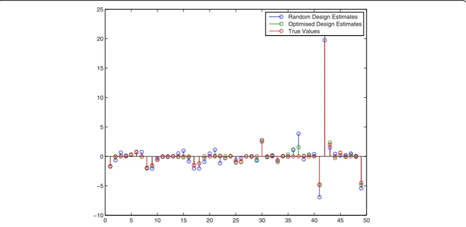
0 5 10 15 20 25 30 35 40 45 50

−10 −5 0 5 10 15 20 25

Random Design Estimates Optimised Design Estimates True Values

methodology (and also demonstrated in two case stud-ies) is that model based experiments are now promin-ently included in the loop and here with the best knowledge that is available, i.e. the most recent estimate [A^;^B] of the parameter vector θ. This yields a more carefully designed parameter estimation problem that allows a more reliable network reconstruction.

One could argue that the linearized system introduces limitations since, of course, the matrices A and B de-pend on the linearization point chosen. Especially if the Jacobi matrix structure changes significantly (in terms of zeros and non-zeros) this can introduce a problem. A remedy would then be to repeat the algorithm for differ-ent values of the state vectorx. However, we emphasize that if there is no connection between node i and j in the network then regardless of the linearization point there will always be a zero in theijth entry. If, therefore, a zero is present in more than one linearization point, the chances are increasingly high that there is indeed no connection between node i and jin the network struc-ture. Our approach contributes to the field of systems biology where the recovery of networks based on stimulus-response data is a central topic that has already caught a lot of attention [6,7]. In systems engineering, model based experimentation has matured substantially but here the design is usually developed for recovery of a set of model parameters in the original non-linear model structure and not for network inference, see e.g. [20] where the input design is formulated in a recursive

manner, meaning that the data and subsequent planning of a new experiment are processed/analysed on-line. Of course, the results presented in the current paper do not include large scale networks with several hundreds of differential equations. But, then, this is not our main message. Rather, we have shown that OID based on dynamic time series of simple perturbation experiments leads to a better overall performance of the parameter estimation algorithm. In addition, the idea of adaptive input design may very well be combined with parameter estimation algorithms that are especially geared for such large scale problems and we think this will almost cer-tainly improve the efficiency of subsequent experimenta-tion and calibraexperimenta-tion as a means to unravel the underlying structure in a network model of a biological system.

Competing interests

The authors declare that they have no competing interests.

Author’s contributions

JD Stigter performed the calculations in the two case studies and wrote the main text. J M wrote most of the introduction and edited the remaining text. Both authors developed the ideas and frame work underlying this paper. Both authors read and approved the final manuscript.

Received: 11 April 2012 Accepted: 19 July 2012 Published: 24 September 2012

References

1. Keurentjes JJB, Angenent GC, Dicke M, Dos Santos VAPM, Molenaar J, vander Putten WH, de Ruiter PC, Struik PC, Thomma BPHJ:Redefining plant

0 500 1000 1500 2000 2500

0 500 1000 1500 2000 2500

Sum of Squared Errors OID

Sum of Squared Errors Random Design

systems biology: from cell to ecosystem.Trends Plant Sci2011, 16(4):183–190.

2. Barabasi AL, Oltvai ZN:Network biology: Understanding the cell’s functional organization.Nat Rev Genet2004,5(2):101-U15.

3. Lucas M, Laplaze L, Bennett MJ:Plant systems biology: network matters. Plant Cell Environ2011,34(4):535–553.

4. Dorf RC:Time-Domain Analysis and Design of Control Systems. Addison-Wesley: Reading, Mass; 1965.

5. Ljung L:System Identification–Theory for the User: Prentice Hall; 1987. 6. Marchal K, De Smet R:Advantages and limitations of current network

inference methods.Nat Rev Microbiol2010,8(10):717–729. 7. Marchal K, Zhao H, Cloots L, Vanden Bulcke T, Wu Y, De Smet R, Storms V,

Meysman P, Engelen K:Query-based biclustering of gene expression data using Probabilistic Relational Models.BMC Bioinformatics2011,12(Suppl. 1):S37. 8. D’Haeseleer P, Liang SD, Somogyi R:Genetic network inference:

fromco-expression clustering to reverse engineering.Bioinformatics2000, 16(8):707–726.

9. Margolin A, Nemenman I, Basso K, Wiggins C, Stolovitzky G, Dalla Favera R, Califano A:ARACNE: An algorithm for the reconstruction of gene regulatory networks in a mammalian cellular context.BMC Bioinformatics 2006,7(1):S7.

10. Faith JJ, Hayete B, Thaden JT, Mogno I, Wierzbowski J, Cottarel G, Kasif S, Collins JJ, Gardner TS:Large-scale mapping and validation of Escherichia coli transcriptional regulation from a compendium of expression profiles.PLoS Biol2007,5:54–66.

11. Menendez P, Kourmpetis YAI, ter Braak CJF, van Eeuwijk FA:Gene Regulatory Networks from Multifactorial Perturbations Using Graphical Lasso: Application to the DREAM 4 Challenge.PLoS One2010, 5(12):e14147. doi:10.1371/journal.pone.0014147.

12. Huynh-Thu VA, Irrthum A, Wehenkel L, Geurts P:Inferring Regulatory Networks from Expression Data Using Tree-Based Methods.PLoS One 2010,5(9):e12776. doi:10.1371/journal.pone.0012776.

13. Bonneau R, Reiss DJ, Shannon P, Facciotti M, Hood L, Baliga NS, Thorsson V: The Inferelator: an algorithm for learning parsimonious regulatory networks from systems-biology data sets denovo.Genome Biol2006, 7(5). doi:10.1186/gb-2006-7-5-r36.

14. Greenfield A, Madar A, Ostrer H, Bonneau R:DREAM 4: Combining Genetic and Dynamic Information to Identify Biological Networks and Dynamical Models.PLoS One2010,5(10):e13397. 10.1371/journal.pone.0013397. 15. Kholodenko BN, Kiyatkin A, Bruggeman FJ, Sontag E, Westerhoff HV, Hoek JB:

Untangling the wires: A strategy to trace functional interactions in signaling and gene networks.Proc Natl Acad Sci USA2002,99(20):12841–12846. 16. Schmid TH, Cho KH, Jacobsen EW:Identification of small scale

biochemical networks based on general type system perturbations. FEBS J2005,272(9):2141–2151.

17. Sontag E:Some new directions in control theory inspired by systems biology.Syst Biol2004,1:9–18.

18. Gardner TS, Faith JJ, Hayete B, Thaden JT, Mogno I, Wierzbowski J, Cottarel G, Kasif S, Collins JJ:Large-scale mapping and validation of Escherichia coli transcriptional regulation from a compendium of expression profiles.PLoS Biol2007,5:54–66.

19. Laub MT, Loomis WF:A molecular network that produces spontaneous oscillations in excitable cells of Dictyostelium.Mol Biol Cell1998, 9(12):3521–3532.

20. Stigter JD, Vries D, Keesman KJ:On adaptive optimal input design: A bioreactor case study.Aiche J2006,52(9):3290–3296.

21. Steinke F, Seeger M, Tsuda K:Experimental Design for Efficient Identification of Gene Regulatory Networks Using Sparse Bayesian Models.BMC Syst Biol2007,1:51.

22. Zavlanos M, Julius AA, Boyd S, Pappas G:Inferring Stable Genetic Networks from Steady-State Data.Automatica2011,47:1113–1122. 23. Franklin G, Powell J, Workman M:DigitalControlSystems. Addison Wesley:

Second Edition; 1990.

24. Walter E, Pronzato L:Qualitative and Quantitative Experiment Design for Phenomenological Models–ASurvey.Automatica1990,26(2):195–213.

doi:10.1186/1756-0500-5-518

Cite this article as:Stigter and Molenaar:Network inference via adaptive optimal design.BMC Research Notes20125:518.

Submit your next manuscript to BioMed Central and take full advantage of:

• Convenient online submission

• Thorough peer review

• No space constraints or color figure charges

• Immediate publication on acceptance

• Inclusion in PubMed, CAS, Scopus and Google Scholar

• Research which is freely available for redistribution