Abstract —Optimal selection of features of Partial Discharge (PD) signals recorded from defects in High Voltage (HV) cables will contribute not only to the improvement of PD pattern recognition accuracy and efficiency but also to PD parameter visualization in HV cable condition monitoring and diagnostics. This paper presents a novel Random Forest (RF)-based feature selection algorithm for PD pattern recognition of HV cables. The algorithm is applied to feature selection of both PD signals and interference signals with the aim of obtaining the optimal features for data processing. Firstly, the experimental data acquisition and feature extraction processes are introduced. PD signals were captured from faults created in a cable to obtain the raw PD data, then a set of 3500 transient PD pulses and a set of 3500 typical interference pulses were extracted, based on which 34 PD features were extracted for further processing. Furthermore, 119 two-dimensional features and 1082 three-dimensional features were generated. The paper then discusses the basic principle of the RF algorithm. Finally, RF-based feature selection was implemented to determine the optimal features for PD pattern recognition. The results were obtained and evaluated with the Back Propagation Neural Network (BPNN) and Support Vector Machine (SVM). Results show that the proposed RF-based method is effective for PD feature selection of HV cables with the potential for application to additional HV power apparatus.
Index Terms—Feature selection, high voltage cables, partial discharge, random forest.
I. INTRODUCTION
ew feature construction and optimal signal feature selection for Partial Discharge (PD) pattern recognition in HV cables are of great importance in two aspects: the identification of the type and severity of PD signals, and the identification of external interference signals. Furthermore, PD pattern recognition accuracy can be improved by effective selection of several new features. In [1], two key features, equivalent time length (T) and equivalent bandwidth (W) were proposed to characterize the fast pulses and slow pulses and Manuscript received October 31, 2018. This work was funded by Key Technological Project of Guangdong Power Grid Corporation (GDKJXM20172769) and National Natural Science Foundation of China (NSFC) 51807072.
Xiaosheng Peng, Fan Yang, Lee Li, Zhaohui Li and Ashfaque Ahmed are with State Key Laboratory of Advanced Electromagnetic Engineering and Technology, School of Electrical and Electronic Engineering, Huazhong University of Science and Technology, Wuhan, 430074, China.
Ganjun Wang and Yijiang Wu are with Zhongshan Power Supply Bureau of the Guangdong Power Grid Corporation, Guangdong, 528400, China.
Chengke Zhou and Donald M. Hepburn are with school of engineering and built environment, Glasgow Caledonian University, Glasgow, G4 0BA, UK.
Alistair J. Reid is with Cardiff School of Engineering, Cardiff University, Queen’s Buildings, The Parade, Cardiff, CF24 3AA, UK.
Martin D. Judd is with High Frequency Diagnostics and Engineering Ltd, Glasgow, G14 0BX, UK.
W. H. Siew is with Department of Electronic & Electrical Engineering, University of Strathclyde, Glasgow, G1 1XW, UK.
these have been widely applied in PD detection and industrial monitoring systems in recent years [2-4]. On the other hand, for the identification of different types of PD signals, recognition accuracy starts to increase rapidly with the dimension of the input features, then fluctuates slightly, before tending to stabilize.
Different types of PD feature have been identified, including waveform features of single pulses, statistical features of PD pulses, spectral features and texture features [5-7]. In addition, based on these traditional features, a large number of combination features can be generated by various mathematical functions. Hence, the feature dimension of a PD pattern could be more than 1000. If all of these features are applied as input parameters, the training of recognition algorithms will be difficult and the recognition efficiency will be low. The relationship between the number of input features and recognition accuracy can be investigated if features can be ranked in order of importance. Hence, optimal feature selection can contribute to the recognition efficiency.
By mining the intrinsic relationship between features and categories, feature selection is conducive to removal of the redundant and irrelevant features and to reduction of the computational complexity of the algorithm [8]. Feature selection methods, such as Relief, Maximize Relevancy and Minimize Redundancy (mRMR), Genetic Algorithm (GA), Rough Set (RS), etc., have been applied in data processing in many fields [9-14]. A comparison of different feature selection methods, including their basic principles, advantages, and disadvantages, is presented in Table I. ‘Relief’ is a feature weighting algorithm, based on which the feature differences both within a given class and across classes are comprehensively evaluated, and feature subsets are selected [9]. The mRMR algorithm is a popular feature selection method for pattern recognition and machine learning, based on the principle of maximizing the correlation between features and classification objectives while minimizing the correlation between features [10]. Both Relief and mRMR have high computational efficiency but relatively poor feature selection accuracy [9-10]. GA is a method of searching the optimal solution by simulating the evolution process of natural organisms [11]. Feature subset selection based on GA needs to be evaluated using the feature evaluation method [11]. Rough Set is an attribute reduction algorithm, based on which redundant features could be removed. It has high computational complexity when a large number of input samples is selected [12]. Feature selection methods based on neural network methods, such as Probabilistic Neural Network (PNN) and Recurrent Neural Network (RNN), are likely to select efficient features from original feature sets [13, 14]. However, due to the characteristic of black box models, PNN and RNN have poor interpretability, and need large data sets for training purposes.
Random Forest Based Optimal Feature Selection for
Partial Discharge Pattern Recognition in HV Cables
Xiaosheng Peng,
Jinshu Li, Ganjun Wang, Yijiang Wu, Lee Li, Zhaohui Li, Ashfaque Ahmed Bhatti, Chengke
Zhou,
Donald M. Hepburn,
Alistair J. Reid,
Martin D. Judd, W. H. Siew
In recent years, feature selection based on the Random Forest (RF) methodology has played an important role in many fields, including gene selection in microarray data analysis [15], feature selection for intrusion detection systems [16] and for spectral data analysis [17]. The important advantages of RF-based feature selection are as follows: 1) RF-based feature selection is carried out automatically during the training process. Owing to the tree structure, it is easy to implement. 2) RF-based feature selection has strong generalization ability and high accuracy due to the two applied random selections in the construction process, which are: random selection of samples and random selection of feature subsets. 3) RF-based feature selection can provide feature ranking results for all the features while most other methods only provide the feature selection subsets. These advantages motivated the authors to develop a RF-based feature selection method for PD signal detection.
TABLEI
COMPARISON OF DIFFERENT FEATURE SELECTION METHODS
Methods Basic
Principle Advantages Disadvantages
Relief
Feature weighting algorithm
High efficiency, suitable for preliminary feature selection
The accuracy is not ideal, ignores feature
redundancy
mRMR
Maximize relevancy minimize redundancy
High efficiency, comprehensive considering
the relevancy and redundancy
The accuracy is not ideal, no ranking results of all features
GA Genetics
mechanism
High efficiency, provides near-optimal solutions in
wide search spaces
Must be combined with feature evaluation methods
Rough Set
Attribute reduction
Removes redundant features, easy to implement
No ranking results of all features, high
computational complexity
PNN Statistical principle
Autonomous learning ability, high efficiency, global optimization capability
Poor interpretability, needs a large data set
to train
RNN
Neural network with loop connections
Autonomous learning ability, suitable for the feature selection of sequence data
Poor interpretability, needs a large data set
to train
RF Feature
permutation
Strong generalization ability, easy to implement, explicit ranking results of all features
High computational complexity
A novel RF-based method for obtaining optimal feature selection for PD pattern recognition of HV cables is presented and validated using laboratory data. Several new PD features are generated, as outlined later, and selected to represent the PD properties. The optimal number of input features is investigated. The result shows that the proposed RF-based method is suitable for PD feature selection in HV cables and has the potential to be extended for application to other HV power apparatus.
II. EXPERIMENTAL DATA ACQUISITION AND FEATURE EXTRACTION
A. Experimental Setup
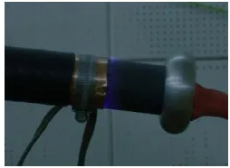
A cross-section showing the structure of the 11kV Ethylene-Propylene-Rubber (EPR) cable is shown in Fig. 1. The five types of artificial defect created in the cable are shown in Fig. 2 and Fig. 3. These defects recreate those typically encountered in the field, but do so under controlled laboratory conditions [18-21]. In EPR insulation, the products of the peroxide decomposition are gases at high temperatures and have some solubility, which may result in the formation of a void defect during and immediately after the curing phase of cable manufacture [19]. Protrusion defects may occur owing to
manufacturing defects or external damage. An interruption in the semiconductor may occur owing to manufacturing defects or installation faults [18]. Incorrect installation of stress cones at end terminations of cables also can lead to PD.
Aluminium core
Inner semiconductor EPR layer Outer semiconductor
Sheath (wound Cu tape) Aluminium armor PVC over sheath
[image:2.612.321.526.97.356.2]21 23 30.5 32.5 34.5
Fig. 1 The construction of the EPR cable sample. Units: mm
Defect type1
3.75 2 0.4
(a)
Defect type2
3.75 2 0.4
(b)
Defect type3
3.75 2 0.4
(c)
Defect type 4
7
(d)
Fig. 2 Defect types: (a) type 1: void in insulation, (b) type 2: protrusion on outer conductor, (c) type 3: floating protrusion, (d) type 4: breach in outer conductor.
Defect type 1 simulates a void in the cable insulation from the outer part of the cable towards the insulation layer. As indicated in Fig. 2(a), a hole is created using a 0.4mm diameter drill and then sealed with copper tape.
Defect type 2 and type 3 simulate metallic protrusion defects. A drill bit was used to bore a hole in the cable, producing the dimensions shown in Fig. 2(b) and Fig. 2(c). The protrusion in type 2 was in contact with the outer semiconductor, the wound copper tape, the aluminum armor and the polyvinyl chloride (PVC) over-sheath. The protrusion in type 3 is floating and not in contact with the aluminum armor and the PVC over-sheath. Defect type 4 simulates a breach in the outer semiconductor of the cable: it is created by removing a 7mm*7mm area from the outer semiconductor, the wound copper tape, the aluminum armor and the PVC over sheath, as shown in Fig. 2(d).
Defect type 5 creates corona discharge around the cable termination by exposing part of the wound copper tape to the air and connecting it to the earth, as shown in Fig. 3.
Fig. 3 Defect type 5: Corona discharge around end termination.
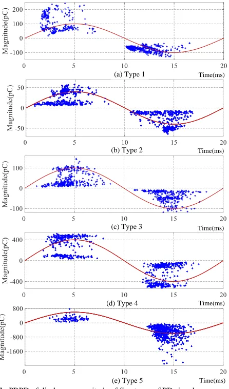
[image:2.612.50.297.258.471.2] [image:2.612.375.502.605.698.2]different from the other 3 types. As a result of the difference in electrical field structure giving rise to the PD, the signals from type 1 and type 5 are quite different from those of the other 3 defects and the signals and are relatively easy to classify. However, as defect type 2 and type 3 have metallic protrusion on outer conductor, PD signals induced in these two defects are relatively similar, which leads to significant difficulty in feature selection and pattern recognition of PD signals.
Next, raw PD data from each defect type were obtained using two industry standard methods, i.e. an IEC 60270 measurement using a coupling capacitor and from measurement using a High Frequency Current Transformer (HFCT) sensor [22]. The coupling capacitor used in the IEC system, Ck, is rated at 100
[image:3.612.56.280.240.356.2]kV and has a capacitance of 1nF ± 10%. The HFCT frequency response is shown in Fig. 4. The bandwidth of the HFCT is from 20kHz to 20MHz.
Fig. 4 HFCT frequency response
PD data was acquired using a LeCroy 104Xi 1GHz digital oscilloscope. The sampling rate of the oscilloscope was 100MS/s and the sampling window 20ms. A diagram of the test setup is shown in Fig. 5.
LeCroy 104Xi, 1GHz r
T
n
Z
k C
m
Z
HFCT
~ AC
Artificial defect Voltage
probe Stress
cone
Cable sample
+25 dB -30
dB Wide-band amplifier
Wide-band attenuator
Earth strap
Fig. 5 PD detection system combining a HFCT and an IEC60270 system.
In order to generate different PD signal intensities, the voltage was increased in steps of 1 kV from 0 to 13 kV. The PD testing voltage and the number of raw data series extracted for 5 types of defects are shown in Table II. As the data acquisition time length is 20ms and the sample rate is 100 MS/s, each data set is about 2M bytes. There are several transient PD pulses within each set of data, especially for defect type 5.
TABLEII
PD TESTING VOLTAGE AND NUMBER OF RAW DATA SERIES FOR EACH DEFECT TYPE Defect
Type 5 kV
6 kV
7 kV
8 kV
9 kV
10 kV
11 kV
12 kV
13 kV SUM Type 1 50 50 50 50 50 50 50 0 0 350 Type 2 0 50 50 50 50 50 54 53 52 409 Type 3 0 51 50 50 26 50 52 61 0 340 Type 4 0 0 50 50 51 52 51 0 0 254 Type 5 0 0 10 10 10 10 10 0 0 50
B. Separation of Interference Signals and PD Signals There are large numbers of interference signals in the raw data obtained from the experiments. Based on the waveform features in the time domain, detected interference signals can be divided into three kinds: white noise, regular interference signal, and random interference signals [22]. Therefore, it is necessary to choose an appropriate method to differentiate the PD signals from the interference signals. The signal identification method based on Synchronous Detection and Multi-information Fusion (SDMF) was applied to the raw data to separate the PD signals from interference signals [22].
Based on IEC 60270 measurement and the SDMF method, a set of 3500 transient PD pulses and a set of 3500 typical interference pulses were extracted from the raw data. There are PD pulses from the 5 defect types in the set of 3500 PD pulses with each type containing 700 PD pulses.
Fig. 6 compares the Phase Resolved PD (PRPD) patterns of identified PD and interference signals from defect type 1 captured by HFCT, in terms of (a) PRPD of maximum voltage of PD pulses and (b) PRPD of equivalent bandwidth of PD pulses. The PRPD of discharge magnitude of PD signals captured by HFCT from the five defect types is shown in Fig.7.
(a)
(b)
Time (ms)
[image:3.612.335.546.314.518.2]PD of Defect Type 1 Interference Signals Time (ms)
Fig. 6 Identified PD and interference signals of defect type 1 captured by HFCT 1: (a) PRPD of maximum voltage (b) PRPD of equivalent bandwidth (W).
C. Feature Extraction and Construction
Based on the set of 3500 PD signals and 3500 interference signals obtained from the five types of artificial defect in the 11kV EPR cable sections, typical PD feature extraction, two-dimensional, and three-dimensional feature construction were carried out.
[image:3.612.52.296.419.540.2] [image:3.612.39.292.660.741.2]Time(ms)
Time(ms)
Time(ms)
Time(ms)
Time(ms)
(a) Type 1
(b) Type 2
(c) Type 3
(d) Type 4
[image:4.612.63.286.50.429.2](e) Type 5
Fig. 7 PRPD of discharge magnitude of five types of PD signals.
TABLEIII
EXTRACTION OF TYPICAL PD FEATURES
Feature type Quantity Features
Position feature 1 phase angle
Amplitude features 5 Peak voltage, mean voltage, root mean square, standard deviation, discharge magnitude Time features 5 signal width, rise time, fall time, T, W
Wavelet feature set 1 6 ED1,ED2,ED3,ED4,ED5,EA5
Wavelet feature set 2 10 Ea1,Ea2,Ea3,Ea4,Ea5,Ed1,Ed2,Ed3,Ed4,Ed5
Other features 7 form factor, crest factor, main frequency, test voltage, polarity, skewness, kurtosis
T-W mapping based on the feature T and feature W, is a well-known method to analyze PD data in the condition monitoring field [1]. Sixteen wavelet features were obtained based on the Discrete Wavelet Transform (DWT). Daubechies wavelets are commonly applied as the mother wavelet for PD data denoising [23, 24]. Based on the PD signals obtained in the laboratory, a comparison of the performance of the mother wavelet between db2 to db 10 was carried out. Db 5 was chosen as the mother wavelet as it was found to achieve the highest correlation with the PD signals captured by the sensor used. The PD signals and interference signals were decomposed into five scales based on DWT. Sixteen wavelet features were then constructed from the coefficients of the resultant wavelet sub-bands. The details of the sixteen wavelet features are shown in Table IV.
TABLEIV
DETAILS OF SIXTEEN WAVELET FEATURES
Feature name Meaning of features
ED1, ED2, ED3, ED4, ED5
Ratio of detail energy for level 1,2,3,4,5 after wavelet decomposition over the energy of original signal
EA5
Ratio of approximation energy over the energy of original signal after wavelet decomposition over the energy of original
signal
Ea1, Ea2, Ea3, Ea4, Ea5
Ratio of approximation energy for level 1,2,3,4,5 over the energy of original signal after wavelet decomposition over the
energy of original signal Ed1, Ed2, Ed3,
Ed4, Ed5
Detail energy for level 1,2,3,4,5 after wavelet decomposition over the energy of original signal
Based on the 34 typical features described previously, 119 two-dimensional features and 1082 three-dimensional features were constructed. There are three methods to construct two-dimensional features: the first is the ratio of two typical features of the same type, the total number of constructed features according to this method is 82, an example is the ratio of two amplitude features (peak voltage/mean voltage). The second method is the square of typical features: the total feature number based on this method 31, an example is the square of position feature (phase angle ^ 2). The third method is the product of polarity and amplitude feature or position feature: the total feature number based on this method is 6, an example is polarity*phase angle. Details of the two-dimensional features are shown in Table V.
TABLEV
CONSTRUCTION OF TWO-DIMENSIONAL PD FEATURES
Quantity Feature type Examples of feature
Ratio of two features
82
ratio of two amplitude features
peak voltage/ mean voltage ratio of two time features signal width/fall time
ratio of two features from
wavelet feature set 1 ED1/ED2
ratio of two features from
wavelet feature set 2 Ea1/Ea2
ratio of skewness and
kurtosis skewness/ kurtosis
ratio of form factor and crest factor
form factor/crest factor
Square of
features 31
square of position features phase angle^2 square of amplitude features peak voltage^2 square of time features signal width^2 square of wavelet features ED1^2
square of skewness or kurtosis
skewness^2 kurtosis^2 square of form factor or crest
factor
crest_factor^2 form_factor^2
Product of two features
6
product of peak voltage and polarity
peak voltage*polarity product of phase angle and
polarity phase angle*polarity
feature, including the ratio of two amplitude features, the ratio of two wavelet features, the square of amplitude features and the square of wavelet features: there are 91 kinds of constructed features based on this method, an example is "peak voltage/mean voltage * polarity". Details of the three-dimensional features are shown in Table VI.
TABLEVI
CONSTRUCTION OF THREE-DIMENSIONAL PD FEATURES
Quantity Feature type Examples of feature
Ratio of three
features 960
ratio of three amplitude features peak voltage/ mean
voltage/root mean square
ratio of three-time features signal width/fall time/T ratio of three features from wavelet
feature set 1 ED1/ED2/ED3
ratio of three features from wavelet
feature set 2 Ea1/Ea2/Ea3
Cube of features 31
cube of position features phase angle^3 cube of amplitude features peak voltage^3 cube of time features signal width^3
cube of wavelet features ED1^3
cube of skewness or kurtosis skewness^3, kurtosis^3
cube of form factor or crest factor crest_factor^3 form_factor^3
Product of three features 91
product of polarity and two-dimensional amplitude features
peak voltage/ mean voltage *polarity product of polarity and ratio of two
features from wavelet feature set 1 ED1/ED2*polarity product of polarity and ratio of two
features from wavelet feature set 2 Ea1/Ea2*polarity product of polarity and square of
amplitude features
peak voltage^2*polarity product of polarity and square of
wavelet features ED1^2*polarity
III. RANDOM FOREST
A. Random Forest -based Feature Selection Algorithm
RF, proposed by Leo Breiman in 2001 [25], is an ensemble machine learning algorithm based on the Decision Tree (DT), which has strong generalization capability and anti-interference ability due to two built-in randomness mechanisms of the algorithm.
The first randomness mechanism is Bagging theory given by Breiman [25]. In order to form one bootstrap training set, bootstrap resampling techniques are applied to extract N samples from the original sample set. The out-of-bag (OOB) sample set of each tree consists of the unselected samples.
The second randomness mechanism is the random subspace method referred by Tin Kam Ho [25] where feature subsets are randomly selected from all features to grow each tree. The best features among the subset rather than all features are elected to split the node of the trees.
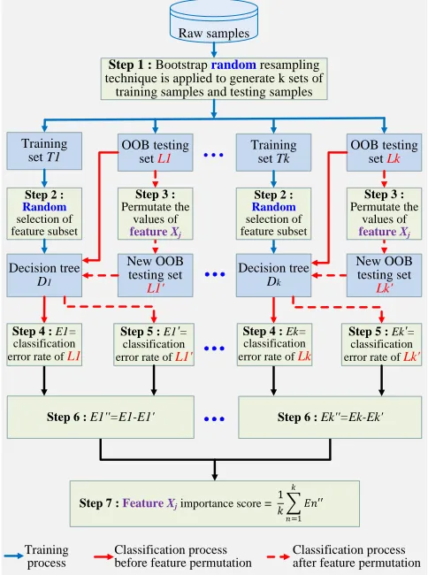
Based on these two randomness mechanisms, RF can be applied to feature importance evaluation and feature selection. The flowchart of RF-based feature selection, as shown in Fig. 8 and discussed below, contains 7 steps.
Step 1:k bootstrap training sets, e.g. T1, and k OOB testing sets, e.g. L1, are generated from the original data by a bootstrap resampling technique.
Step 2: For each bootstrap training set, a decision tree is built. Feature subsets are randomly selected from all features at each
node and the best feature in the subset is taken to split the tree nodes. k decision trees, Di (i=1, 2… k), are trained by the k
bootstrap training sets.
Step 7 : Feature Xjimportance score = OOB testing
set L1
Training set T1
Raw samples
Decision tree
D1
New OOB testing set
L1'
Step 6 :E1''=E1-E1' Step 6 : Ek''=Ek-Ek'
Step 2 :
Random
selection of feature subset
OOB testing set Lk
Training set Tk
Step 1 : Bootstrap random resampling technique is applied to generate k sets of
training samples and testing samples
Decision tree
Dk
New OOB testing set
Lk'
Step 5 :E1'=
classification error rate of L1'
Step 5 : Ek'=
classification error rate of Lk'
Training process
Classification process before feature permutation
Classification process after feature permutation
1
𝑘 𝐸𝑛′′
𝑘
𝑛=1
Step 3 :
Permutate the values of
feature Xj
Step 3 :
Permutate the values of
feature Xj
Step 4 : E1=
classification error rate of L1
Step 4 : Ek=
classification error rate of Lk
Step 2 :
Random
[image:5.612.318.560.94.419.2]selection of feature subset
Fig. 8 Flowchart of RF-based feature selection
Step 3: Permutate the values of feature Xj in all OOB testing
sets, keep the values of other features unchanged and get new OOB testing sets, e.g. L1’,with particular feature permutation.
Step 4: Classify the corresponding OOB testing set Li (i=1,
2… k) with the corresponding decision tree Di and calculate the
error rate Ei (i=1, 2… k).
Step 5: Classify the corresponding new OOB testing set Li’
(i=1, 2… k) with the corresponding decision tree Di and
calculate the error rate E i’ (i=1, 2… k).
Step 6: Calculate the difference in the error rate of Ei and Ei’
(i=1, 2… k) to get the error rate difference E i’’ (i=1, 2… k). Step 7: Add the k error rate difference results E i’’ (i=1, 2… k), and the average value of the results is the importance score of the feature Xj.
In Step 3, feature permutation is difficult to understand and is the key to the RF-based feature selection, so further interpretation of feature permutation is added here.
The commonly applied feature importance measure in RF is permutation importance, which is based on the changes of classification error rate between the intact OOB samples and those with particular feature permutation. In order to measure the importance of a specific feature Xj, the values of Xj in the
OOB samples are randomly changed. In other words, the features of Xj are permutated. An example of feature
[image:5.612.48.299.142.411.2]interference signal. The original values of feature Xj of sample
1 to sample 6 are a1, a2…a6 respectively. After the feature
permutation, the values of Xj of sample 1 to sample 6 are turned
into a5, a4…a3 respectively. The original
values of feature Xj
The values of Xj
after the feature permutation
Feature Permutation Defect type
sample1 ... sample2
... sample3
... sample4
... sample5
... sample6
... type 1
type 2
type 3
type 4
type 5
noises
a1 ... a2 ... a3 ... a4 ... a5 ... a6 ...
a5 ... a4 ... a1 ... a2 ... a6 ... a3 ... Fig. 9 Feature permutation of feature Xj
The more the classification error rate decreases after feature permutation and the higher the score of feature importance of Xj,
the more important the feature.
RF has three key parameters, the number of features in the feature subset (mtry), the criterion to split the nodes and number
of trees (Tk). In this paper, the reference values of mtry are
obtained based on the calculation formula of mtry in [25, 26],
and the optimal value of mtry is gained by traversals. The two
most commonly applied criteria for splitting nodes are information gain and Gini index. In-depth theoretical analysis of these two criteria is carried out in [27], which indicates that these two criteria only show disagreement in 2% of all these cases. Based on these theoretical results, the classification effects of these two criteria are evaluated using laboratory data and the optimal splitting criterion is determined. It is observed that 500 trees are sufficient to meet the classification requirement [16] and an excessive number of trees would waste computing resources. Here, the value of Tk is determined
according to the OOB error rate.
B. Flowchart of RF-Based Optimal PD Feature Selection
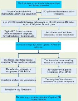
The flowchart of the RF-based optimal PD feature selection, shown in Fig. 10, is divided into three stages: (a) experimental data acquisition and feature extraction, (b) RF-based optimal PD feature selection and (c) evaluation of results of optimal PD feature selection.
The first stage is experimental data acquisition and feature extraction. As outlined above, five types of artificial defect were made in 11kV EPR cable and tested. An IEC measurement system and an HFCT were used to obtain the raw PD data, from which, 3500 typical interference pulses and 3500 transient PD pulses were extracted. The number of PD samples for each class is 700. Additional information on this experiment was published in [22]. As discussed, typical PD feature extraction and two-dimensional and three-dimensional feature construction were applied to the PD and interference pulses. 34 PD features were extracted, 119 two-dimensional and 1082 three-dimensional features were generated, respectively: each pulse has, in total, 1235 features.
The second stage is RF-based optimal PD feature selection, which is an RF process and a feature importance measure process. The details of the steps are shown in section A of part I.
The validation with pattern recognition: SVM, BPNN 5 types of artificial defects manufacture and raw data acquisition
The feature importance ranking
results for PD and interference signals results for 5 types of PD signalsThe feature importance ranking
The validation with pattern recognition: SVM, BPNN The second stage: RF-Based optimal PD feature
selection
Two-dimensional and three-dimensional feature construction
Correlation analysis and visualization
PD pulses and interference pulses extraction
The analysis of input features dimension for pattern recognition
Several new key PD features
a set of 3500 typical interference pulses and a set of 3500 transient PD pulses (a set of 700 pulses for each type)
Typical PD feature extraction: position features of the pulses, wavelet features of the pulses, etc.
The first stage: experimental data acquisition and feature extraction
The third stage: results evaluation of optimal PD feature selection
Fig. 10 Flowchart of RF-based optimal feature selection for PD pattern recognition.
The third stage is results evaluation of optimal PD feature selection, which is divided into the following two aspects:
1)The results evaluation of optimal feature selection based on PD signals and interference signals. The features importance ranking results are analyzed by Support Vector Machine (SVM) and Back Propagation Neural Networks (BPNN) based pattern recognition methods. Correlation analysis of the top 20 features is carried out. Two-dimensional visualization analysis of specific features is developed and compared with the traditional T-W mapping method to receive the key features which can characterize PD properties.
2)The results evaluation of optimal feature selection based on PD signals from 5 defect types. The feature importance ranking results for the PD signals from the 5 fault types are also calculated by SVM and BPNN. The optimal dimension of input features for pattern recognition based on experimental data is investigated to improve the recognition efficiency.
IV. RESULTS OF RF-BASED OPTIMAL FEATURE SELECTION FOR PDSIGNALS AND INTERFERENCE SIGNALS
The set of 3500 PD pulses and of 3500 interference pulses, each of which has 1235 features associated with it, is to be investigated. The reference values of mtry are 11 and 36
respectively, based on the calculation formula of mtry in [25, 26]
and the adjacent values of the reference values are crossed for further optimization. The results show that the optimal value of mtry is 33. Following the theoretical analysis method in [27], the
[image:6.612.314.564.51.376.2]accuracy of the PD data were analyzed and compared. The results show that the Gini index criterion has better classification accuracy. Based on the method in [16], the variation of OOB error rate with the number of trees Tk is
obtained by traversals. The results show that both the training efficiency of the RF algorithm and the classification accuracy are the highest when the value of Tk is optimal, i.e. at 350.
A. The Importance Ranking Results for Features of both PD and Interference Signals
The results of optimal feature selection for PD signals and interference signals, using the RF-based method, are shown in Table VII.
TABLEVII
RANKED FEATURE IMPORTANCE SCORES FOR PD AND INTERFERENCE SIGNALS
Ranking Feature Importance
scores
1 Ea4/Ed1 0.033 355
2 W/rise time/T 0.028 900
3 Fall time/W/signal width 0.026 687
4 T/W 0.026 667
5 Fall time/signal width/W 0.024 471
6 EA5/ED1/ED2 0.022 248
7 Signal width/W/T 0.022 245
… …. …
20 Ea2/Ed1 0.015 577
21 W/rise time/fall time 0.015 564
… … …
30 W 0.013 338
78 T 0.002 219
160 ED2 0.001 119
166 Ed1 0.001 006
868 skewness 0.000 501
869 kurtosis 0.000 459
874 ED3 0.000 409
880 Ea3 0.000 398
886 magnitude 0.000 380
… … …
The results show that the effective features for recognizing PD signals and interference signals are mainly those features which characterize the signal width and those which are related to wavelet features of PD pulses. The features characterizing the signal width mainly relate to features like T, W, rise time and fall time. Effective wavelet combination features of PD pulses include Ea4/Ed1, EA5/ED1/ED2 and so on.
B. Validation with Pattern Recognition Based on Features Importance Ranking Results
SVM- and BPNN-based pattern recognition methods were applied to evaluate the validity of RF-based optimal feature selection according to pattern recognition accuracy. SVM has three key parameters: kernel function, penalty factor C and kernel function parameter γ [28]. For the validation study in this work, Radial Basis Function (RBF) is chosen as the kernel function, based on the quantitative relationship of input data and features; the Grid-Search and Cross-Validation method are applied to the optimization of C and γ [28]. A widely used three-layered BPNN is adopted in this paper. Although the number of nodes in the hidden layer is the most important parameter of a BPNN, as it affects the accuracy and efficiency of BPNN-based pattern recognition [29], there is no available theory on how the number of nodes in the hidden layer should be chosen. To compensate for this, several variations in number of nodes were compared to achieve the best signal classification
accuracy [29].
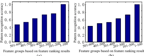
The top 600 ranked features were selected and divided into 6 groups: each group containing 100 features. The six groups of features were applied to the pattern recognition algorithm respectively. The recognition results, in which the ranking results of RF-based feature importance are used as abscissa, are shown in Fig. 11.
0.0 0.2 0.4 0.6 0.8 1.0
Feature groups based on feature ranking results
(a) (b)
0.0 0.2 0.4 0.6 0.8 1.0
Pat
tern
reco
g
n
it
io
n
a
ccu
racy
Pat
tern
reco
g
n
it
io
n
a
ccu
racy
[image:7.612.316.559.136.232.2]Feature groups based on feature ranking results
Fig. 11. Pattern recognition results of PD and interference signals: (a) SVM-based results, (b) BPNN-based results.
From Fig. 11, the recognition accuracy of SVM and BPNN increases with the level of ranking of feature importance. The recognition accuracy of the first feature group (1-100) under SVM and BPNN is 52.13% and 58.72% higher than that of the sixth group (501-600) respectively, from which it is clear that the RF-based feature selection method is an effective way to select appropriate features for analysis of PD signals and interference signals from HV cables.
C. Visualization Analysis Based on Features Importance Ranking Results
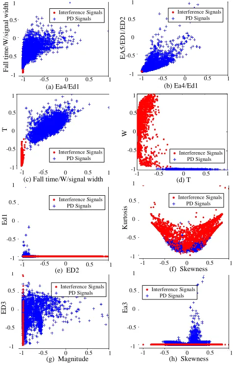
Correlation analysis of the top features was carried out and specific features with high importance scores and low correlation were selected for visual evaluation, as shown in Fig. 12.
To assist with an effective comparison analysis, normalization of all the features was carried out, i.e. adjusting the range of the parameters to -1 to 1. Because of the strong correlation between the second feature and the third feature, the first feature “EA4/ED1" and the third feature "Fall time/W/signal width" were selected for visualization in Fig. 12(a). The result of a typical T-W mapping method is shown in Fig. 12(d). Several low-ranking features, such as skewness, kurtosis, ED3 and Ea3, were also selected for comparison, as shown in Fig. 12(e)-(h). The ranking and importance scores of these features are shown in Table VII.
The conclusions that can be drawn from the data presented are as follows:
1) The accumulation degree of interference signals in Fig. 12(a) and Fig.12(b) are better than that under T and W in Fig.12(d), which indicates that "EA4/ED1","Fall time/W/signal width" and "EA5/ED1/ED2" are more likely to perform better than T and W for recognition of interference signals. Therefore, "EA4/ED1","Fall time/W/signal width" and "EA5/ED1/ED2" can serve as key features to differentiate PD signals and interference signals and to suppress interference signals.
2) The aggregation range of PD signals under "EA4/ED1" and "Fall time/W/signal width" is wider than that under T and W, which can provide analysis and recognition of different types of PD signals. Therefore, "EA4/ED1" and "Fall time/W/signal width" can be applied for monitoring and visualization of different types of PD signals.
with high ranking results, i.e. Fig.12(a)-(d), are better than those based on features with low ranking results, i.e. Fig. 12(e)-(h),. The boundaries between PD signals and interference signals are clear in Fig.12(a)-(d) while the indicators of PD signals and interference signals in Fig. 12(e)-(h) overlap, which indicate the efficiency of the RF-based ranking of features. Based on Fig. 12 (a)-(c), it should be possible to set a specific threshold to separate effectively PD signals from interference signals.
ED
3
(g) Magnitude
-1 -0.5 0 0.5 1
-1 -0.5 0 0.5 1 Interference Signals PD Signals Ea 3
(h) Skewness
-1 -0.5 0 0.5 1 -1 -0.5 0 0.5 1 K urt os is
(f) Skewness
-1 -0.5 0 0.5 1
-1 -0.5 0 0.5 1 Interference Signals PD Signals Ed 1
(e) ED2
-1 -0.5 0 0.5 1
-1 -0.5 0 0.5 1 Interference Signals PD Signals T
(c) Fall time/W/signal width
-1 -0.5 0 0.5 1
-1 -0.5 0
0.5
1
-1 -0.5 0 0.5 1
-1 -0.5 0 0.5 1 (d) T W Interference Signals PD Signals F al l ti m e /W /s igna l w idt h (a) Ea4/Ed1
-1 -0.5 0 0.5 1
-1 -0.5 0 0.5 1 Interference Signals PD Signals EA 5 /ED 1 /ED 2 (b) Ea4/Ed1
-1 -0.5 0 0.5 1
[image:8.612.54.292.161.534.2]-1 -0.5 0 0.5 1 Interference Signals PD Signals Interference Signals PD Signals Interference Signals PD Signals
Fig. 12 Results of visual verification of PD signals and interference signals.
The PD signals and interference signals used in this paper were obtained under laboratory conditions. Future work will focus on optimal feature selection based on typical interference and PD signals obtained in practical industrial situations.
V. RESULTS OF RF-BASED OPTIMAL FEATURE SELECTION FOR FIVE DIFFERENT TYPES OF PDSIGNALS
A. Feature Importance Ranking Results forPD Signals from Five Defect Types
The RF-based optimal feature selection results for PD signals from 5 defect types are shown in Table VIII. The results show that the wavelet combination features of PD pulses, having higher ranking, are effective features for distinguishing PD signals from different defect types.
According to Table II, the information relating the PD test
voltage and the number of data sets for different defects, type 1 defects have a set of 50 PD pulses when the test voltage is 5 kV. Similarly, type 2 defects have a set of 52 PD pulses when the test voltage is 13 kV. Therefore, 7.27% of the PD samples are distinguishable from the original samples only by the "test voltage" feature. Table VIII indicates that "test voltage" achieves a high ranking among all features, which is consistent with the result obtained. This analysis strongly supports the validity of the RF-based method for optimal feature selection.
The "phase angle * polarity" feature is an effective feature for PD signal identification and is widely implemented in the analysis of PRPD. In Table VIII, "Phase angle * polarity" is seen among the high importance score rankings, which is in line with established research results and so strongly supports the RF-based method for feature selection.
TABLEVIII
RANKED FEATURE IMPORTANCE SCORES FOR PD SIGNALS FROM FIVE DEFECT TYPES
Ranking Feature Importance
scores
1 Ed5/Ed3/Ea5 0.019 68
2 Ed3/Ea4/Ea2 0.015 57
3 Ed5/Ed3/Ea1 0.015 40
… … …
7 Test voltage 0.013 88
8 Ed5/Ea2/Ed3 0.013 49
… … …
13 Phase angle*polarity 0.011 09
14 Ed3/Ea1/Ea4 0.010 83
… … …
B. Validation of Pattern Recognition Based on Features Importance Ranking Results
Consistent with the method in section B of part IV, SVM- and BPNN-based pattern recognition methods were applied to evaluate the validity of RF-based feature importance ranking results for PD signals from 5 defect types. The accuracy of pattern recognition results are shown in Fig. 13.
0.3 0.4 0.5 0.6 0.7 0.8 0.9 0.3 0.4 0.5 0.6 0.7 0.8 0.9 (a) (b) Pa tt ern rec o g n it io n a ccu racy
Feature groups based on feature ranking results
Pat tern reco g n it io n a ccu racy
[image:8.612.357.521.250.363.2]Feature groups based on feature ranking results
Fig. 13 Pattern recognition results for PD signals from 5 defect types: (a) SVM-based results, (b) BPNN-based results.
From Fig. 13, it can be observed that the change of the recognition accuracy coincides with the level of feature importance ranking results. With increasing importance of the level of ranking of features, there is an upward trend to the recognition accuracy of SVM and BPNN. The recognition accuracy of the sixth feature group under SVM and BPNN is 28.82% and 24.37% lower than that of the first group.
C. Analysis of Input Features Dimension for Pattern Recognition Based on Features Importance Ranking Results
[image:8.612.314.562.460.556.2]In general, there is a consistent trend in change in recognition accuracy of both the BPNN-based method and the SVM-based method. The recognition accuracy increases rapidly as the number of input features increases from zero, then almost plateaus in a stable state. At very high numbers of input features, the recognition accuracy fluctuates slightly but, overall, shows a slight downward trend. Therefore, to ensure optimum operation of the pattern recognition methods, the optimal feature dimension for pattern recognition should be determined. This improves efficiency of the determination by removing redundant features, saving on system resources, reducing time and cost of data processing, as well as ensuring high recognition accuracy. Fig. 14 suggests that, based on the set of 3500 PD samples, the optimal value of feature dimensions for differentiating PD signals from 5 defect types is around 100.
0 50 100 150 200 250 300
The number of input features
0.5 0.6 0.7 0.8 0.9 1
SVM BP
Ac
cur
acy
Fig. 14 PD pattern recognition accuracy versus the number of input features.
VI. CONCLUSION
This paper proposes a novel RF-based method for determining the optimal features for PD pattern recognition from faults in HV cables. The results are tested using experimental PD data from defects created in HV cable sections. The conclusions are summarized as follows:
As demonstrated by the BPNN and SVM validation results, the RF-based feature selection method is an effective way to select appropriate features for analysis of PD signals and interference signals from HV cables and for differentiating PD signals from different defect types.
Based on the presented RF-based feature selection results for PD signals and interference signals, the effective features are the signal width related features and wavelet features, e.g. T, W, rise time, signal width, Ea4/Ed1, EA5/ED1/ED2.
Based on the presented RF-based feature selection results for PD signals from five defect types, the wavelet combination features of PD pulses, high in the ranking results, are effective features for distinguishing PD signals from different defect types.
As the number of features applied to the recognition algorithm increases the recognition accuracy first increases rapidly then levels off, but tending to decrease slightly. The number of features at which stability is attained is around 100. Therefore, based on the data presented in this paper, the proposed dimension for pattern recognition of PD signals from 5 defect types is 100.
Based on the presented RF-based feature selection and feature visualization analysis, the feature combination of "EA4/ED1" and "Fall time/W/signal width" shows better performance than the traditional T-W mapping method. This
conclusion needs to be further evaluated using a wider range of PD and interference samples.
The PD signals and interference signals used in the paper were collected from laboratory samples and under laboratory conditions. In order to extend the set of key features to include those encountered in the field through on-line cable monitoring systems, future work will include further studies on optimal feature selection based on typical interference and PD data obtained in industrial applications.
REFERENCES
[1] G. C. Montanari, A. Cavallini, and F. Puletti, “A new approach to partial discharge testing of HV cable systems,” IEEE Elect. Insul. Mag., vol. 22, no. 1, pp. 14-23, Apr. 2006.
[2] Y. Lin, “Using K-Means Clustering and Parameter Weighting for Partial-Discharge Noise Suppression,” IEEE Trans. Power Del., vol. 26, no. 4, pp. 2380-2390, Sep. 2011.
[3] B. Qi, C. Li, B. Geng, and Z. Hao, “Severity Diagnosis and Assessment of the Partial Discharge Provoked by High-Voltage Electrode Protrusion on GIS Insulator Surface,” IEEE Trans. Power Del., vol. 26, no. 4, pp. 2363-2369, Sep. 2011.
[4] G. Luo, D. Zhang, Y. Koh, K. Ng, and W. Leong, “Time–Frequency Entropy-Based Partial-Discharge Extraction for Nonintrusive Measurement,” IEEE Trans. Power Del., vol. 27, no. 4, pp. 1919-1927, Jul. 2012.
[5] K. Firuzi, M. Vakilian, B. T. Phung, and T. R. Blackburn, “Partial Discharges Pattern Recognition of Transformer Defect Model by LBP & HOG Features,” IEEE Trans. Power Del., pp. 1-1, Oct. 2018.
[6] W. J. K. Raymond, H. A. Illias, and A. H. A. Bakar, “High noise tolerance feature extraction for partial discharge classification in XLPE cable joints,” IEEE Trans. Dielectr. Elect. Insul., vol. 24, no. 1, pp. 66-74, Mar. 2017.
[7] V. P. Darabad, M. Vakilian, B. T. Phung, and T. R. Blackburn, “An efficient diagnosis method for data mining on single PD pulses of transformer insulation defect models,” IEEE Trans. Dielectr. Elect. Insul., vol. 20, no. 6, pp. 2061-2072, Dec. 2013.
[8] J. Xiao, Y. Xiao, A. Huang, D. Liu, and S. Wang, “Feature-selection-based dynamic transfer ensemble model for customer churn prediction,” Knowl. Inf. Syst., vol. 43, no. 1, pp. 29-51, Apr. 2015. [9] Z. Cai, J. Gu, and H. Chen, “A New Hybrid Intelligent Framework for
Predicting Parkinson’s Disease,” IEEE Access, vol. 5, pp. 17188-17200, Aug. 2017.
[10] H. Peng, F. Long and C. Ding, “Feature selection based on mutual information criteria of max-dependency, max-relevance, and min-redundancy,” IEEE T. Pattern Anal., vol. 27, no. 8, pp. 1226-1238, Jun, 2005.
[11] H. Uguz, “A two-stage feature selection method for text categorization by using information gain, principal component analysis and genetic algorithm,” Knowl.-Based Syst., vol. 24, no. 7, pp. 1024-1032, Sept, 2011. [12] J. Liang, F. Wang, C. Dang and Y.Qian, “A group incremental approach
to feature selection applying rough set technique,” IEEE Trans. Knowl. Data Eng., vol. 26, no. 2, pp. 294-308, Oct. 2014.
[13] C. Lee, and Y. Shen, “Optimal Feature Selection for Power-Quality Disturbances Classification,” IEEE Trans. Power Del., vol. 26, no. 4, pp. 2342-2351, Jun. 2011.
[14] T. Rückstieß, C. Osendorfer and P.V.D.Smagt, “Sequential Feature Selection for Classification,” Lect. Notes. Artif. Int., vol. 7106, pp. 132-141, Dec. 2011.
[15] M. B. Kursa, “Robustness of Random Forest-based gene selection methods,” BMC Bioinformatics, vol. 15, no. 1, pp. 8, Jan. 2014. [16] M. A. M. Hasan, M. Nasser, S. Ahmad, and K. I. Molla, “Feature
selection for intrusion detection using random forest,” J. Inf. Secur., vol. 7, no. 03, pp. 129, Apr. 2016.
[17] B. H. Menze, B. M. Kelm, R. Masuch, U. Himmelreich, P. Bachert, W. Petrich, and F. A. Hamprecht, “A comparison of random forest and its Gini importance with standard chemometric methods for the feature selection and classification of spectral data,” BMC Bioinformatics, vol. 10, no. 1, pp. 213, Jul. 2009.
characteristics from insulation defects in 11kV EPR Cable. Presented at 17th Int’l. Sympos. High Voltage Eng.
[19] M. Brown, “Performance of Ethylene-Propylene rubber insulation in medium and high voltage power cable,” IEEE Trans. Power App. Syst.,
vol. 102, no. 2, pp. 373-381, Feb. 1983.
[20] H.A. Illias, M.A. Tunio, A.H.A. Bakar, H. Mokhlis and G. Chen, "Partial discharge phenomena within an artificial void in cable insulation geometry: experimental validation and simulation", IEEE Trans. Dielectr. Electr. Insul., vol. 23, no. 1, pp. 451-459, Mar. 2016.
[21] O. E. Gouda1, A. A. ElFarskoury, A. R. Elsinnary and A. A. Farag, “Investigating the effect of cavity size within medium voltage power cable on partial discharge behavior,” IET Gener. Transm. Dis., vol. 12, pp. 1751-8687, Jul. 2017.
[22] X. Peng, J. Wen, Z. Li, G. Yang, C. Zhou, A. Reid, D. M. Hepburn, M. D. Judd, and W. H. Siew, “SDMF based interference rejection and PD interpretation for simulated defects in HV cable diagnostics,” IEEE Trans. Dielectr. Elect. Insul., vol. 24, no. 1, pp. 83-91, Feb. 2017. [23] X. Ma, C. Zhou, and I. J. Kemp, "Automated wavelet selection and
thresholding for PD detection," IEEE Elect. Insul. Mag., vol. 18, no. 2, pp. 37-45, Mar. 2002.
[24] X. Zhou, C. Zhou, and I. J. Kemp, "An improved methodology for application of wavelet transform to partial discharge measurement denoising," IEEE Trans. Dielectr. Electr. Insul., vol. 12, no. 3, pp. 586-594, Sept. 2005.
[25] L. Breiman, “Random forests,” Mach. Learn., vol. 45, no. 1, pp. 5-32, Oct. 2001.
[26] H. Kawakubo, and H. Yoshida, “Rapid feature selection based on random forests for high-dimensional data,” Expert Syst. Appl., vol. 40, pp. 6241-6252, Mar. 2012.
[27] L. E. Raileanu, and K. Stoffel, “Theoretical comparison between the gini index and information gain criteria,” Ann. Math. Artif. Intel., vol. 41, no. 1, pp. 77-93, May. 2004.
[28] L. Hao and P. L. Lewin, “Partial Discharge Source Discrimination using a Support Vector Machine”, IEEE Trans. Dielectr. Electr. Insul., vol. 17, no.1, pp. 189 -197, Feb. 2010.