Some Multicolor Ramsey Numbers Involving Cycles

(1)

Rochester Institute of Technology

RIT Scholar Works

Theses Thesis/Dissertation Collections

5-2015

Some Multicolor Ramsey Numbers Involving

Cycles

David E. Narvaez

Follow this and additional works at:http://scholarworks.rit.edu/theses

Recommended Citation

(2)

Some Multicolor Ramsey Numbers Involving Cycles

APPROVED BY

SUPERVISING COMMITTEE:

Dr. Stanis law P. Radziszowski, Advisor Department of Computer Science Rochester Institute of Technology

Date

Dr. Edith Hemaspaandra, Reader Department of Computer Science Rochester Institute of Technology

Date

Dr. Ivona Bez´akov´a, Observer Department of Computer Science Rochester Institute of Technology

(3)

Some Multicolor Ramsey Numbers Involving Cycles

by

David E. Narv´

aez

THESIS

Presented to the Department of Computer Science of the Golisano College of Computing and Information Sciences

in Partial Fulfillment of the Requirements for the Degree of

Master of Science in Computer Science

Rochester Institute of Technology

(4)

Abstract

Some Multicolor Ramsey Numbers Involving Cycles

David E. Narv´aez, M.S.

Rochester Institute of Technology, 2015 Supervisor: Dr. Stanis law P. Radziszowski

Establishing the values of Ramsey numbers is, in general, a difficult task from the computational point of view. Over the years, researchers have developed methods to tackle this problem exhaustively in ways that require intensive computations. These methods are often backed by theoretical results that allow us to cut the search space down to a size that is within the limits of current computing capacity.

This thesis focuses on developing algorithms and applying them to gen-erate Ramsey colorings avoiding cycles. It adds to a recent trend of interest in this particular area of finite Ramsey theory. Our main contributions are the enumeration of all (C5, C5, C5;n) Ramsey colorings and the study of the

(5)

Chapter 1

Introduction

Finite Ramsey theory studies guaranteed properties of partitions of graphs with a finite number of vertices. Unlike infinite Ramsey theory, where most of the important results are presented in the form of existential state-ments, in finite Ramsey theory we are interested in specific values known as Ramsey numbers, which are the orders of related extremal graphs. Because one of our goals is to compute these numbers, this field is also known as com-putational Ramsey theory. Partitioning the set of edges of a graph can also be regarded as “coloring” the edges. Ramsey numbers concerning partitions into k sets are also called k-color Ramsey numbers and are called multicolor Ramsey numbers for k > 2. As a concrete example, it is known that any complete graph on 25 or more vertices, when partitioned into two subgraphs, will yield a partition where either the first graph contains a complete graph on 4 vertices, or the second graph contains a complete graph on 5 vertices.

(8)

analytical or done by hand. With the advent of computers, researchers were able to use these to find exact values for larger cases. This also helped improve on the analytical results and find better bounds. For instance, the concrete example mentioned above is due to Brendan McKay and Stanis law Radzis-zowski [MR95], who developed novel algorithms for efficiently traversing trees of graphs and use them for related problems. Today, research in computational Ramsey theory lies on the boundary between pure discrete mathematics and computer science, with one often improving on the results of the other.

To illustrate the difficulty of the task of determining the exact value of certain Ramsey numbers, it is useful to consider the following citation from Joel Spencer [Spe94]

“Erd˝os asks us to imagine an alien force, vastly more powerful than us, landing on Earth and demanding the value of R(5,5) or they will destroy our planet. In that case, he claims, we should marshal all our computers and all our mathematicians and attempt to find the value. But suppose, instead, that they ask for R(6,6). In that case, he believes, we should attempt to destroy the aliens.”

(9)

from an insightful theoretical result that will drastically cut down the number of cases to analyze. After this initial step, we are then able to create programs that will perform suitable computations.

The structure of this thesis is as follows: Chapter 2 introduces the theory behind Ramsey numbers and related fields, Chapter 3 deals specifically with monochromatic cycles in graph colorings. Chapters 4 and 5 use the algorithms introduced in Chapter 3 to explain how we generated (C5, C5, C5)

colorings and to describe our strategy to approach the problem of finding

(10)

Chapter 2

Background

This chapter introduces the notation that will be used throughout this thesis. While the central topic of this work is Ramsey theory, some other fields of discrete mathematics are used to support the many tools developed in order to solve the problem in hand. A good reference for more in-depth study of many of the concepts described in this chapter is Bollob´as book on Extremal Graph Theory [Bol04].

2.1

General Graph Theory

For a graph G = (V, E), V and E are the set of vertices and edges, respectively. Define the functions n(G) = |V| and e(G) =|E|. We may also useV andE as functions of a graph, whereV (G) (respectively,E(G)) denotes the set of vertices (respectively, edges) of a graphG. The numbern(G) is also referred to as the order of G and we denote by _Gn the set of graphs of order

n. The neighborhoodN(v, G) of a vertex v in a graphGis the set of vertices

v0 such that {v, v0_{} ∈}_E_{, and the degree of that vertex is} _d₍_{v, G}_{) =}_|_N₍_{v, G}₎_|_.

(11)

Kn is the complete graph on n vertices, Kn −e is a Kn without one

edge and Ki,j is a complete i by j bipartite graph. Cn is a cycle of length

n and Pn is a path on n vertices. As it is customary, (see, e.g. [Rad94]) we

define the binary operation H ∪G to be the disjoint union of two graphs H

and G and the operation H +G to be H∪G with the addition of all edges betweenH and G. nG stands for G∪G∪. . .∪G

| {z }

n-times

.

Two graphsG1 = (V1, E1) andG2 = (V2, E2) are isomorphic if and only

if there is a bijectionφ :V1 →V2 such that {φ(v1), φ(v2)} ∈E2 ⇔ {v1, v2} ∈

E1 for all v1, v2 ∈ V1. Intuitively, this can be interpreted as two graphs that

have the same “shape” but possibly different vertices. An automorphism is an isomorphism from a graph to itself, i.e., a permutation of the vertex labels such that the set of edges remains the same. Because the composition of two automorphisms is also an automorphism, the automorphisms of a graph form a group:

Definition 2.1 (Automorphism Group). Aut (G) is the group of all

automor-phisms of a graph Gunder the composition operation.

For simplicity, we extend the notation for permutations of elements to elements to permutations of sets to sets. For a permutationφ:A→B and a setS ∈2A_{, the notation} _φ₍_S_{) is defined as the set} _{φ₍_s₎_|s _∈_S_}_.

Given a subset V0 of the vertices of a graph G = (V, E), the graph induced by V0 in G is the graph G0 = (V0, E0) where E0 is the set of edges in

(12)

G[V0] denote the graph induced by V0 in G. We say a graph G contains a subgraph isomorphic to H = (VH, EH) (or, more informally, contains a copy

of a graph H) when there is an injective function φ : VH → V such that

{vi, vj} ∈ EH ⇒ {φ(vi), φ(vi)} ∈ E. Notice that the image of φ defines a

subsetV0 inV, but the graph induced byV0 inGis not necessarily isomorphic to H. The graph G−v is the result of removing a vertex v ∈ V (G) from a graphG, together with all edges{v, w} ∈E(G) or, equivalently,G−v denotes the graph G[V (G)\ {v}]. When two graphs H = (V, EH) and G = (V, EG)

share the same set of vertices, it makes sense to use the notation H ⊆ G to indicate H is a subgraph of G if one takes these graphs to be collections of sets {u, v} with u, v ∈V.

A subgraph ofG that is isomorphic toKk is called a clique of order k.

The complement of a graph G, denoted G, is the graph formed by the edges “missing” in G, i.e. G = (V,{{v1, v2} |v1, v2 ∈V, v1 6=v2} \E). A clique

of size k in the complement of a graph G is called an independent set of

G. The independence number α(G) of a graph G is the order of the largest independent set in G. The Tur´an number of a graphG for graphs of order n, denoted τ(G, n), is the maximum number of edges among graphs of order n

that contain noG as a subgraph.

2.2

Ramsey Theory

(13)

belong to the field of extremal graph theory. One property of interest is the presence or absence of a specific subgraph and this is the primary focus of Ramsey theory.

Definition 2.2 (Ramsey Numbers). Given k graphsG1, G2, . . . , Gk, the

mul-ticolor Ramsey numberR(G1, G2, . . . , Gk) is the smallest integerN such that,

in every assignment of k colors to the edges of a complete graph of order at leastN, there is a color 1≤i≤k such that the graph formed by the edges of the i-th color contains a copy ofGi.

For brevity, when the graphs Gi are all equal to a graph G, we write

this number asRk(G). Ramsey’s theorem [Ram30] states that these numbers

exist and are computable. The dynamic survey by Radziszowski [Rad94] is the standard reference for an extensive overview of the advances in this field. A k-coloring of the set of edges of a graph G = (V, E) is a function

C : E → {1,2, . . . , k}. A (G1, G2, . . . , Gk;n) coloring is a k-coloring of a

complete graph of ordernsuch that thei-th color contains noGi as a subgraph.

To simplify our notation, we will refer to



G, G, . . . , G | {z }

k

;n



colorings asG-free

k-colorings of order n. It is easy to see that any graph on n vertices can be regarded as a complete graph on n vertices whose edges are painted in two colors, the second one being “transparent,” thus a (G1, G2;n) coloring can

also be called a (G1, G2;n) graph. If Gis a graph coloring using k colors, the

(14)

Notice that the Ramsey numberR(G1, G2, . . . , Gk) can then be defined as the

smallest integerN such that no (G1, G2, . . . , Gk;N) coloring exists.

A typical example of Ramsey theory is the following problem, which has become part of mathematical folklore [Gar97]:

Problem 2.1 (Problem E 1321, The American Mathematical Monthly, June

- July, 1958). Prove that at a gathering of any six people, some three of them are either mutual acquaintances or complete stranger to each other.

This can be formulated in terms of graph. This formulation appeared as a problem in the William Lowell Putnam mathematical competition:

Problem 2.2 (William Lowell Putnam Mathematical Competition, 1953,

Question A2). The complete graph with 6 points and 15 edges has each edge colored red or blue. Show that we can find 3 points such that the 3 edges joining

them are the same color.

Solving this problem is equivalent to proving that the Ramsey number

R(K3, K3) is at most 6. To prove that R(K3, K3) = 6, the graph in Figure

2.1 shows the well-known 2-coloring of the complete graph on 5 vertices that contains no monochromatic triangle.

(15)

Figure 2.1: Witness graph for R(K3, K3)>5

2.3

nauty

It is not known whether or not there exists a polynomial-time algo-rithm to test whether two graphs are isomorphic or not [GJ79]. On the other hand, it is easy to see that this problem is crucial for graph theory research. The development of good algorithms to solve this problem efficiently is then of great importance and has received much attention in the past decades.

no automorphisms, yes? [MP14] is a collection of software tools and a C library to deal with graph isomorphisms and automorphism groups. It was first published by Brendan McKay in 1981 and has been used in several other approaches to establish the exact values of Ramsey numbers [MR95].

At the heart of the automorphism detection innauty is the concept of a canonical labeling. As defined in [Pip08], the canonical labeling of a graph

Gis a graphG0, isomorphic toG, representing the whole isomorphism class of

(16)

canonical labelings G0₁ and G0₂ and then compare these graphs for equality.

nauty’s strategy to find the canonical labeling of a graph is to search for a

permutation of the labels of the input graph by traversing a search tree of all possible labelings. The efficient traversal of such a large search space is based on several heuristics that prune parts of the search space. As is often the case with heuristics, these work particularly well for certain types of graphs and may perform poorly for other types of graphs. Other graph isomorphism algorithms that are based on exploring a search tree are found in saucy [DLSM04] and

Bliss [JK07].

Traces [Pip08] is another algorithm that is distributed with nauty

which improves some of the original heuristics. In particular, it removes some

of nauty’s original sensitivity to the node invariant used to prune the search

tree. Node invariants are important components in the heuristics innautythat can make a great difference when used correctly, but the mastering of these requires advanced knowledge of the internals of the algorithms. Traces then tries to remove the burden of the know-how from the user by avoiding such a tight dependency between the pruning heuristics and the node invariants.

The concept of canonical labelings is also useful when dealing with a large number of graphs because it allows us to “deduplicate” graph databases by keeping only one representative of the isomorphism classes in it. This fea-ture was critical to keep our dataset of (C5, C5, C5;n) colorings within

(17)

the shortg and shortmc1 tools that are part of nauty.

While our use ofnauty for the enumeration of (C5, C5, C5;n) colorings

was limited to external tooling, we usednauty extensively as a library in our approach to establishing the value of R(C4, C4, K4). For this problem, the

automorphism groups are essential to many of the definitions, as explained in Chapter 5.

1_shortmc_{is part of a yet unpublished extension to}_nauty_{developed by Brendan MacKay}

(18)

Chapter 3

Colorings Avoiding Cycles

In this chapter we focus on the task of coloring the set of edges of a graph with k colors so that the graphs induced by the each color contain no cycles of a given length. We then say a graph can besplit intokcolors avoiding

Cm if this task can be achieved. Cycle-free Ramsey colorings have received

much attention in recent years, as shown by the many results compiled in Radziszowski’s [Rad11] survey on this particular area of Ramsey theory.

We employ two strategies to generate k-colorings that avoid cycles in each of the k colors: direct coloring of edges (Section 3.2) and extending good

k-colorings by adding a vertex (Section 3.3). In both strategies, a fundamental piece is the cycle detection algorithm described in the next section.

3.1

Cycle Detection

(19)

version of this algorithm, this will be enough to return with a positive answer. In the “search” version of the algorithm, the cycle detected is removed from the queue and added to the list of cycles in the solution.

The na¨ıve implementation of this algorithm will naturally find all 2n

directed paths in a cycle of length n, which increases the processing time. To improve over this implementation, an idea from Floyd’stortoise and hare

algorithm [Flo67] can be adopted. The key is to assume the first vertex in each path is the vertex with the largest label in the path. This reduces du-plicates to exactly two per cycle, which is a significant speedup over the na¨ıve implementation when the number of cycles is large.

3.2

Coloring the Edges

One way to generate colorings that avoid cycles of length m is to list all edges that form cycles of lengthm in a graph and finding combinations of these edges such that every set of edges in an m-cycle is intersected at least once and at mostm−1 times by each color. Notice that, ifEis the set of edges that participate in any cycle of length m in a graph G, then we would need to perform the intersection check described above for every partition {E1,E2}

ofE. Yet, a significant number of checks can be avoided by using the concept of the Tur´an number: since we know that a valid partition of E must satisfy

|E1| ≤ τ(Ck, n) and |E2| ≤ τ(Ck, n) and because |E1|+|E2| = |E|, we must

have

(20)

In the case of odd cycles, the Tur´an numberτ(C2l+1, n) is known to be

j

n2

4

k

, so 3.1 can be applied as

|E| −

n2

4

≤ |E1| ≤

n2

4

.

3.2.1 SAT Formulation

An alternative way to formulate the 2-coloring problem is to assign a Boolean variable to every edge in the graph and calculate the setCof all cycles of lengthm in it. Then, for every cycle C in C, a Boolean expression

m

_

i=1

f(C, i)∧

m

_

i=1

f(C, i)

is formulated, wheref(C, i) is the variable assigned to the i-th edge of C. A truth assignment of the variables can then be trivially mapped to a proper coloring of the complement of the given graph.

We implemented this alternative solution using the PicoSAT [Bie08] library, version 959. In practice, this implementation is faster than the direct enumeration of all possible edge colorings for certain graphs, but not all of them.

3.2.2 Constraint Programming Formulation

(21)

n vertices can be represented by n2 _variables _e

i,j that can take integer values

between 0 and k. Here, 0 means the edge corresponding to that variable is not in the graph. Then a constraint satisfaction solver can assign integers to these variables subject to constraints like

m−3

_

i=0

evσ(i),vσ(i+1) =6 evσ(i+1),vσ(i+2)

!

∨evσ(m−2),vσ(m−1) 6=evσ(k−1),vσ(0)

for every m-subset {v0, v1, . . . , vm−1} of vertices and every permutation σ of

the set {0,1, . . . , k−1}. These constraints guarantee that, in any permuta-tion of m-subsets of vertices, at least two consecutive edges do not have the same color. We implemented this formulation using the Ben-Gurion University Equi-propagation Encoder (BEE) [MC12].

3.3

Extending Good Colorings

If we have the list of allCm-freek-colorings of ordern, we can generate

allCm-freek-colorings of ordern+1 by adding a vertexvand joining it with all

the n previous vertices, then coloring these n new edges withk colors so that no cycle of length k is formed in any color. Specifically, for every candidate coloring C of the n new edges, we require that for every pair of vertices u, w

that are endpoints of a monochromaticPm−1 inG with all edges colored with

the i-th color, we haveC({v, u})6=i orC({v, w})6=i.

Despite the fact that there arekn _{candidate colorings for this process,}

(22)

Chapter 4

(

C

5

, C

5

, C

5

;

n

)

Colorings

This chapter details our search for all (C5, C5, C5;n) colorings. It is

known that R(C5, C5, C5) = 17, so this search would only be carried out up

to graphs of order 16, which is within the reach of current computing power. The lower bound 17 ≤ R3(C5) is derived from the fact that the

fol-lowing blow-up construction [JMW13] yields a Cn-free k-coloring of order

2k−1₍_n₋_{1) for any odd} _n1_:

1. Given a fixednandkcolors, construct a complete graph onn−1 vertices using the first color.

2. For c := 2,3, . . . , k−1, duplicate the current graph and color all edges that join vertices of the two copies using the c-th color.

In [YR92b], Yuansheng and Rowlinson showed that R3(C5) = 17 by

executing an exhaustive, computer-aided search for colorings of the comple-ment of C5-critical graphs of order 17. In this context, a critical graph on n

vertices stands for a graph of ordern that isC5-free and adding any edge to it 1_{The use of this construction in the context of Ramsey numbers of cycles of odd length}

(23)

[image:23.612.148.490.132.311.2]

(a)K4 (b) 2K4+K4,4 (c) 4K4+ 2K4,4+K8,8

Figure 4.1: Blow-up construction forC5 and k= 3

completes a cycle of length 5. To further reduce the search space, the authors show that the only graphs that need to be checked are those that:

1. Have at least 46 edges (the total number of edges, divided by 3), since it is possible to assume, without loss of generality, that the first color of the (C5, C5, C5; 17) coloring that will be generated is the one with the

largest amount of edges.

2. Have no independent set of order 9, since R2(C5) = 9 [CS71].2

There are 52 graphs that meet these criteria, and there is no way to color the complement of these graphs using two colors to produce a (C5, C5, C5; 17)

graph, which establishes that R3(C5) = 17.

2_{This is easy to verify by combining a cycle detection algorithm with} _nauty_’s _complg

(24)

At this point it is important to distinguish between the exhaustive search done in [YR92b] and the exhaustive listing of (C5, C5, C5;n) colorings

[image:24.612.161.471.236.376.2]

we present in this report: It is possible to generate all critical graphs without listing all (C5, K9;n) graphs explicitly, as shown in [YR92a].

Figure 4.2: Witness colorings forR(C5, C5) = 9

We can apply the concepts of Sections 3.2 and 3.3 to generateC5-free

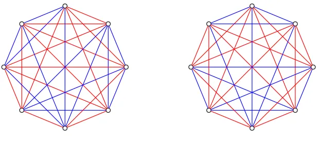
3-colorings for 1≤n ≤16. For instance, we can take aC5-free graph and color

the complement of this graph with two colors in a way that avoids cycles of length 5. Figure 4.3 shows an example of two (C5, C5, C5; 8) colorings generated

using this method. Also, with the complete set of (C5, C5, C5;n) colorings for

some n, we can generate all (C5, C5, C5;n+ 1) colorings by adding a vertex

(25)

[image:25.612.205.427.116.264.2]

Figure 4.3: Two of the 12,586 ways to split the complement of this graph of order 8 such that there are no cycles of length 5.

4.1

R

3

(

C

3

)

vs

R

3

(

C

5

)

Because R3(C3) = R3(C5) = 17, it is interesting to compare the

be-havior of the number of colorings relevant to each of these Ramsey numbers. By looking at Table 4.4 we can see several differences between the two families of colorings. An immediate observation one can make is that there are many more (C5, C5, C5;n) colorings than (C3, C3, C3;n) colorings for any given n.

Furthermore, despite the fact that the behavior of the number of colorings for both types is that it increases monotonically up to some value ofn, then starts decreasing monotonically, the value ofn that yields the maximum number of colorings differs between the colorings forC3 and C5.

4.2

Open Science Grid

(C5, C5, C5;n) colorings for 13 ≤ n ≤ 16, which are shown in Table

(26)

Number of Vertices (C3, C3, C3;n) (C5, C5, C5;n)

6 330 2 349

[image:26.612.176.456.114.293.2]

7 3 829 54 927 8 50 391 679 876 9 500 023 3 713 104 10 2 646 593 14 092 138 11 4 821 244 43 945 253 12 1 929 792 140 033 320 13 78 892 448 105 921 14 115 1 142 773 713 15 2 1 844 045 362 16 2 1 701 746 176

Table 4.4: Counts of weakly isomorphic colorings for (C3, C3, C3;n) and

(C5, C5, C5;n). The number of (C3, C3, C3;n) colorings were calculated by

Radziszowski [Rad14] and independently verified by the author.

workflow of this project, the monolithic file containing all (C5, C5, C5; 12)

col-orings was split and each part was processed separately by several computing nodes. The output of these processes was then merged together in a hierarchi-cal way using nauty’s shortmc tool. The orchestration of this workflow was done through the Pegasus project [DSS+_05].

4.3

Description of the Colorings

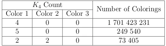
The large number of colorings obtained as a result of this process makes it challenging to provide a succinct description of the dataset. We decided to provide a description in terms of the number of K4 subgraphs found in each

(27)

K4 Count

Number of Colorings Color 1 Color 2 Color 3

4 0 0 1 701 423 231

5 0 0 249 540

[image:27.612.177.452.116.192.2]

2 2 0 73 405

Table 4.5: Tally of (C5, C5, C5; 16) colorings by number ofK4’s per color

of the colorings.

Figure 4.6 illustrates each type of coloring described in Table 4.5. All colorings with five K4’s in one color have exactly 30 edges in that color. The

subgraph induced by that color corresponds to four K4’s mutually attached

through an additionalK4. We will call this graph 4K4×. In the case of colorings

with twoK4’s in the first color and twoK4’s in the second color, the vertex sets

forming theseK4’s are disjoint and their union is the whole set of vertices. For

colorings with four vertex-disjoint K4’s in the first color, there are 29 graphs

induced by that color. We will call this set K. An easy way to describe some of the graphs in K is to notice that the complement of any graph G on 16 vertices with 4K4 ⊆ G is a subgraph of 4K4, which has a C5-free 2-coloring.

Since both 4K4 and 4K4× are C5-free, we have the following lemma:

Lemma 4.1. If G is a graph of order 16 with 4K4 ⊆G⊂4K4×, then there is

a (C5, C5, C5; 16) coloring that induces a monochromatic G in some color.

From Lemma 4.1 we can deduce that 10 of the 29 graphs in question are fourK4’s mutually attached by any of the 10 graphs on 4 vertices that are

(28)

(a) FourK4’s (b) FiveK4’s (c) Two K4’s in one color

and two K4’s in another

[image:28.612.131.481.125.271.2]

color

Figure 4.6: Sample (C5, C5, C5; 16) colorings according to our classification.

on the following transformation:

Definition 4.1 (Shrink of G). Let G = (V, E) be a graph of order 16 such that 4K4 ⊆Gand letP={P0, P1, P2, P3}be a partition of V such that G[Pi]

is a K4. The graph S(G) = (P, E0) is defined such that {Pi, Pj} ∈ E0 if and

only if there exists a pair of vertices u0, v0 ∈ V (G) such that u0 ∈ Pi, v0 ∈ Pj

and {u0_{, v}0_{} ∈}_E₍_G_).

Intuitively, we shrink the fourK4’s inG and represent the connections

between the original vertex sets as edges in the new graph. Notice that, if

G∈K, for every edge{Pi, Pj} ∈E(S(G)) there is exactly one pair of vertices

u0, v0 ∈V (G) that satisfies the definition above because, if there was another pair {u00_{, v}00_} _{such that} _u00 _∈ _P

i, v00 ∈ Pj and {u00, v00} ∈ E(G) then G would

have a cycle of length 5.

(29)

hand, counting the number of graphsG∈K whose shrink is isomorphic to H

seems to require a case-by-case analysis of all the graphs on 4 vertices.

4.4

Bounds on

R

4

(

C

5

)

The lower bound 33≤R4(C5) comes from the fact that we can generate

aC5-free 4-coloring on 32 vertices by using theblow-up construction explained

before. For the upper bound, the formula in [Rad94] isRk(C5)<

√

18k_k_!

10 , which

yields R4(C5) ≤ 158. This inequality, which originally appears in [Li09], is

derived from the inequality Rk(C5)−1 <1 +

√

18k(Rk−1(C5)−1) which is

stronger, but can only be used if the value ofRk−1(C5) is known. Since in our

case we knowR3(C5) = 17, this last inequality implies R4(C5)≤137.

As in the previous section, we analyze what the number of K4’s in a

(C5, C5, C5, C5; 32) coloring could be. The blowup construction already yields

a coloring with eight K4’s in one color. Furthermore, the complement of a

graph obtained from eight copies ofK4’s mutually attached through aC5-free

graph on 8 vertices is a subgraph of the complement of 8K4, so it has aC5-free

3-coloring. Since any C5-free graph on 8 vertices has, at most, two K4’s, this

(30)

Chapter 5

R

(

C

4

, C

4

, K

4

)

This chapter focuses on the problem of establishing the value of the Ramsey number R(C4, C4, K4). Before this work, this value was known to

be at least 20 [DD11] and at most 22 [XSR09]. As in Section 3.3, our strat-egy was to generate (C4, C4, K4; 20) colorings by extending (C4, C4, K4; 19)

colorings that have a particular structure. This structure guarantees that failing to generate any (C4, C4, K4; 20) colorings by exhaustively trying to

extend all (C4, C4, K4; 19) colorings obtained would imply that there are no

(C4, C4, K4; 20) colorings at all, proving that R(C4, C4, K4) = 20.

5.1

Previous Bounds

The lower bound was established by taking a graph on 18 vertices that contains no cycle of length 4 and coloring the complement of this graph avoiding cycles of length 4 in the second color and the complete graph of order 4 in the third color. The original graph on 18 vertices was described first in 1989 by Clapham, Flockhart and Sheehan in [CFS89]. The proof for the upper bound is also based on [CFS89], since it uses the values forτ(C4,22) to prove

(31)

two colors avoiding C4 in both of them. The reasoning is very similar to the

one used in the forthcoming Theorem 5.1.

Later in 2011, Dybizba´nski and Dzido showed (Figure 4 of [DD11]) a graph coloring on 19 vertices that contains no cycles of length 4 in the first two colors and no complete graph of order 4 in the third color. The Ramsey number R(C4, C4, K4) must then be at least 20.

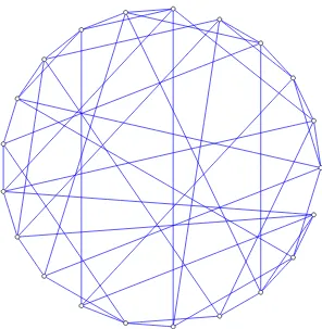
One graph mentioned in [CFS89] that is of particular importance for Theorem 5.1 was originally described in the context of cycles of length 4 by Erd˝os, R´enyi and S´os in 1966 [ERS66]. The vertices in this graph correspond to points in the projective plane P G(2, k), for a prime power k. There are

k2₊_k_{+ 1 of these points. An edge between vertices (points)} _A _and_B _{(in our}

case, A 6= B to avoid loops) exists if and only if A is in the dual line of B. From this definition and the fact that there is a single line passing through any two points in a projective plane, one can deduce that if edges AC, BC,

AC0 and BC0 exist in this graph, then the dual line ofC is the dual line ofC0

soC =C0. In particular, this means that there is no cycle of length 4 in this graph. Fork = 22, this graph of order 21 is shown in Figure 5.1. By removing one vertex of degree 4 from this graph, one obtains a graph of order 20 with no cycle of length 4. These two graphs are unique witnesses forτ(C4,21) and

(32)

[image:32.612.166.462.219.522.2]

(33)

5.2

The Structure of the Third Color

Our strategy is based on the following theorem about graphs induced by the third color of any (C4, C4, K4; 20) coloring:

Theorem 5.1. Let G be a (C4, C4, K4; 20) coloring. Then there are two

non-adjacent vertices in G[3] whose degree is 11.

Proof. As in the solution of Theorem 5.1 in [XSR09], we note that

∆ (G[3]) ≤ 11: Indeed, because R(C4, C4) = 12 [Rad94], the complement of

the graph induced by the neighborhood of any vertex inG[3] can be of order at most 11. LetD11be the set of vertices inG[3] whose degree is 11. We claim

that|D11| ≥4. Then, take 4 vertices fromD11. BecauseG[3] is K4-free, these

vertices do not induce a complete graph in G[3], so there must be 2 vertices that are non-adjacent.

To prove our claim, assume by contradiction, that |D11| ≤ 3. It is

easy to see that Lemma 4.4 in [CFS89] guarantees the existence of a vertex of degree 4 inG[3], so

e(G[3]) ≤

4 +|D11| ×11 + (19− |D11|)×10

2

=

194 +|D11|

2

≤98 On the other hand, τ(C4,20) = 46 [CFS89] and G[1] and G[2] have

noC4, so

e(G[3]) =

20 2

−e(G[1])−e(G[2]) ≥190−2×46 = 98

so e(G[3]) = 98 and G[1] is isomorphic to the unique witness graph for

(34)

2 colors such that the first color contains noC4 and the second color contains

no K4 [Rad14], a contradiction.

In view of Theorem 5.1, we can choose two non-adjacent verticesuand

v of degree 11 in the third color of a (C4, C4, K4; 20) coloring and remove u.

We are then left with a (C4, C4, K4; 19) coloring Gwhere the neighborhood of

vertexv inG[3] induces a graph X of order 11 with noK3 and the rest of the

vertices (not adjacent to v) induce a graphY of order 7 with no K4. Both X

and Y have the additional property that their complement can be split into 2 colors avoidingC4. Furthermore, while the edges between X and Y will be

determined by this extension process, the graph induced by the vertex v and the vertices ofY depends only onY. This meansY also has the property that the complement of the graph obtained by adding a disconnected vertex to it can also be split into 2 colors avoidingC4. We can now “reconstruct”G from

its pieces v, X and Y by choosing graphs X and Y from the sets G11 and G7

defined in Table 5.2 and defining the set of edges between X and Y so that noK4 is created and the complement of the resulting graph can be split into

2 colors avoiding C4.

G7 can be easily generated by combiningnauty’sgengandpickg tools

to list all non-isomorphic graphs on 8 vertices and pick those with minimum degree 0, then discarding those that either contain K4 or whose complement

cannot be split into 2 colors avoiding C4; and finally dropping one vertex of

degree 0 in each one of them. One could, in theory, generateG11using a similar

(35)

Set Description Size

G7 K4-free graphs of order 7 to

which we can add one vertex and the complement of the result-ing graph will have a 2-colorresult-ing avoiding C4

587

G11 K3-free graphs of order 11 whose

complement can be split into 2 colors avoidingC4

575

G13 All graphsGinduced by the third

color of all (C4, C4, K4; 13)

color-ings with ∆ (G) = 11

[image:35.612.188.448.114.294.2]

243997

Table 5.2: Sets of graphs used to reconstruct a (C4, C4, K4; 19) coloring

11. Instead, one can exploit the fact that the set of all (K3, C6; 11) colorings1

is a superset of G11, because R(C4, C4) = 6.

Figure 5.3 illustrates one graph of 19 vertices that can be obtained via this process. The dashed edges join the vertex v to every vertex in X. The dotted edges join vertices ofY with feasible neighborhoods of X.

5.3

Feasible Neighborhoods

Lety be a vertex in Y. The graph G0 induced inG[3] by v, y and the vertices in X is a K4-free graph of order 13 whose complement can be split

into 2 colors avoiding C4, so it must be in the set of graphs obtained by

ex-tracting the graph induced by the third color of every (C4, C4, K4; 13) coloring.

Conversely, for every graph H induced by the third color of a (C4, C4, K4; 13) 1_{This set is available at}

(36)

[image:36.612.169.465.138.283.2]

Figure 5.3: A graph produced by the extension process

coloring such that ∆ (H) = 11, its vertices can be mapped to v, y and the vertices ofX by selecting a vertex of degree 11 to bev, its neighborhood to be the set of vertices ofX and the remaining vertex to be y. After this mapping is found, one additional property about X can be noted: the set of vertices

N(y, H) defines, in X, a set of vertices to which a vertex of Y can be joined. To exploit this mapping, we define an additional set G13 of graphs of

order 13 and maximum degree 11 that are induced by the third color of a (C4, C4, K4; 13) coloring. For every graph H = (VH, EH) inG13 we define the

tuple Ψ (H) = (vH, yH, XH, φH) where:

• vH = min{h∈VH |d(h, G) = 11}

• yH is the vertex inVH that is not adjacent tovH.

(37)

nauty [MP14].

• φH is the (unique) isomorphism between the graph induced in H by the

vertices in VH \ {vH, yH} and XH.

Notice that Ψ is well defined: if Ψ (H) = (vH1, yH1, XH1, φH1) and

Ψ (H) = (vH2, yH2, XH2, φH2), from the definition of vH, it is clear that vH1 =

vH2, and this defines yH1 = yH2; also, from the definition of φH, the

func-tion φH1φ

−1

H2 is an isomorphism between XH2 and XH1, so it must be that

XH2 =XH1 and φH1 =φH2.

Intuitively, by considering all tuples Ψ (H) that associate an H ∈ G13

with a graphX ∈G11, one can find a collection C0(X) of subsets of vertices of

Xto which a vertexy∈Y can be joined when reconstructing a (C4, C4, K4; 19)

coloring. But C0(X) may not be the complete collection of subsets that are feasible neighborhoods of a vertexy: one needs to take into account that any subset of vertices ofX that is symmetric to a subset inC0(X) is also a feasible neighborhood for a vertex y. Formally, for a canonically labeled graph X = (VX, EX) inG11, a subsetVX0 ⊆VX is called acanonically feasible neighborhood

if there is a graph H in G13 such that Ψ (H) = (vH, yH, φH, X) and VX0 =

{φX(φH(v))|v ∈N(yH, H)}. We denote by C0(X) the set of all canonically

feasible neighborhoods of in X. The set C(X) of feasible neighborhoods in graph X is then the set of all subsets {φ(v)|v ∈V_X0 } of VX for some φ ∈

(38)

With this description, it is possible to implement an algorithm that will calculate, for every canonically labeled graph X ∈ G11, the sets C(X)

and C0(X) by first iterating over all graphsH ∈G13 finding the tuples Ψ (X)

that define all subsets inC0(X) and then applying every automorphism of the graphXto the vertices of every subset inC0(X) to generate a (possibly larger) set C(X). We used nauty to perform the mappings required to calculate the tuples in Ψ (H) and to calculate the automorphism groups of the graphs X

to generate the complete set of feasible neighborhoods. An alternative way of doing this is to iterate over every canonically labeled graphX ∈G11, adding a

vertex v adjacent to every vertex inX and an additional vertexy, then joining

ywith every possible subset of vertices inXand looking up the resulting graph of order 13 in G13: if the lookup is successful, the subset to which ywas joined

belongs to C(X).

5.4

Compatible Neighborhoods

The previous section was concerned with what can happen when we add one vertex as we try to extend a graph in G11 to a graph on 19 vertices

that is a valid third color for some (C4, C4, K4; 19) coloring. We now take one

more step in that direction: Consider two vertices y1 and y2 in Y that are

joined to subsets VX1 and VX2 of vertices in X. Obviously, VX1 ∈ C(X) and

VX2 ∈C(X), but this is not enough to guarantee the graphs of order 14 formed

by this setup when y1 and y2 are adjacent and non-adjacent, respectively, is

(39)

testing for this condition requires expensive computations, our goal is to test for simpler conditions that will discard graphs that are not valid third colors, without false negatives. Our choice of conditions is the following:

(K4) G must not containK4 as a subgraph.

K6

Gmust not contain an independent set of order 6.

(4K1∪K3) No subset of 7 vertices can induce the graph 4K1∪K3 inG.

(3K1∪2K2) No subset of 7 vertices can induce the graph 3K1∪2K2 in G.

The reason for condition (K4) is obvious from the purpose of this

con-struction. The reason for condition K6

is that R(C4, C4) = 6 so if G

con-tained an independent set of order 6, at least the complete graph on 6 vertices in the complement of Gcannot be split into 2 colors avoidingC4. The reason

for conditions (4K1∪K3) and (3K1∪2K2) is that the complement of these

graphs, shown in Figure 5.4, cannot be split into 2 colors avoiding C4. This

fact, while easy to verify computationally, can be stated as a lemma and proven analytically. For this, we rely heavily on another lemma about the coloring of

K6 −e avoiding monochromatic C4’s, which is discussed in Appendix A.

Lemma 5.2. There is no blue/red coloring of the complements of the graphs

4K1∪K3 and 3K1∪2K2 that avoids monochromatic C4’s.

Proof. The exact same reasoning applies to both graphs so, in the following,

(40)

there is a blue/red coloring of G that avoids monochromatic C4’s. Let v be

a vertex of minimum degree in G. Then the graph G−v is isomorphic to

K6−e and, by Lemma A.1, there is only one way to color this graph avoiding

monochromaticC4’s. Label the remaining 6 verticesw0, w1, w2, w3, x, y so that

xyis the missing edge andw0w1w2w3 is a monochromaticP4. Because the two

colors in theC4-free coloring of K6−eare symmetric, we can assume without

loss of generality that:

• There are at least as many vwi blue edges as there are red vwi edges,

otherwise we can exchange the colors.

• The path w0w1w2w3 is blue (and the path w2w0w3w1 is red), otherwise

we can relabel these vertices.

• The edges w0x and w1y are also blue, otherwise we can exchange the

labels x and y.

From the blue pathsw0w1w2,w1w2w3,w0xw4 and w1yw2 one can see that the

collection W = {{w0, w2},{w1, w3},{w0, w3},{w1, w2}} is such that, if vwi

and vwj are blue and {wi, wj} ∈ W, then we would have a blue C4. Clearly,

if three or more of the vwi edges were blue, some set {wi, wj} ∈ W would be

such that vwi and vwj are both blue and a blue C4 would be formed. Then

there are exactly two blue vwi edges and two red vwi edges. We then have

4 2

− |W| = 2 possible choices of blue edges between v and the wi vertices:

(41)

[image:41.612.182.446.84.274.2]

(a) 4K1∪K3 (b) 3K1∪2K2

Figure 5.4: Forbidden subgraphs

we have a red cyclevw2w0w3; orvw2 andvw3 are blue, in which case the edges

vw0 and vw1 are red and we would have a red cycle vw0w3w1. In any case,

we reach a contradiction, so there is no blue/red coloring of G that avoids a

monochromaticC4.

One can then generate a compatibility matrix of all subsets inC(X) for the cases when y1 and y2 are adjacent and non-adjacent. These matrices are

useful even beyond the point where 2 vertices have been added to extend the (C4, C4, K4; 12) coloring because, at the point where we add the k-th vertex

to this construction and consider a candidate neighborhood for it, one can quickly check it is compatible with thek−1 neighborhoods chosen before for the other vertices.

5.5

Extension Process

(42)

of order 19 that have the structure described in Theorem 5.1.

In adding vertices to a graph in G11 to obtain a graph on 19 vertices

that is a valid third color for some (C4, C4, K4; 19) coloring, we mention the

following two strategies that can be used:

1. Adding a single vertex in every step. In its simplest form, this strategy supposes we have added k vertices to the initial graph in G11, so at the

k + 1-st step we have a graph or order 12 +k if we take into account the vertex v adjacent to all the vertices of the original graph. For the

k+ 1-st vertex, we need to try all possible connections to the previous k

vertices that have been added and then pick a feasible neighborhood that is compatible with the rest of the neighborhoods chosen so far. A nice property of this strategy is that one can assume that, for some ordering of the list of feasible neighborhoods, their assignment to the vertices of the extended graph are in non-decreasing order. Intuitively, this means that, at a successful termination of this extension process, the vertices of some graphY ∈G7 will have been “discovered” in some order defined by

the compatible neighborhoods attached to them. A drawback of blindly selecting the adjacency of thek+1-st vertex with respect to thekvertices previously added is that one may end up with a graph of order k+ 1 that is not a subgraph of any graph in G7.

2. Appending each graph Y ∈G7 and joining each of the 7 vertices of the

(43)

neighborhood is chosen for the next vertex with the condition that the new neighborhood must be compatible with every neighborhood selected for the previous vertices. This approach improves over the first approach in the sense that we know a priori that the 7 vertices added to the graph will yield a graph with the structure described in Theorem 5.1. It also suggests an easy scheme for problem partitioning in order to run the extension process in parallel: every pair of graphs (X, Y) can be checked independently using a total of|G11| · |G7|processes. The drawback of this

approach is that no order can be assumed for the feasible neighborhoods assigned to the vertices of Y. Also, in a naive implementation of this approach a graph of order n < 7 that is a subgraph of several graphs in G7 will be checked many times for the same combination of feasible

neighborhoods.

In both strategies, the graph that is generated in every step is checked for conditions (K4), K6

, (4K1 ∪K3) and (3K1∪2K2) described in Section

5.4. If the graph fails to satisfy any of these conditions, the extension of X

withY using the current combination of neighborhoods is aborted. It might be that the complement of the final graph generated once feasible neighborhoods of X are chosen for each one of the 7 vertices of Y can not be split into two colors avoiding C4 in both of them. Thus, this additional final check is

(44)

While the description of the strategies above involves feasible neighbor-hoods, a way to reduce the number of combinations to try is to use canonically feasible neighborhoods. The following theorem allows us to pick the first fea-sible neighborhood from the (possibly smaller) set C0(X):

Theorem 5.3. coloring Let G be a graph obtained by the extension process

described above, composed of a vertex v, a graph X ∈ G11 and a graph Y ∈

G7. Let X0, X1, . . . , X6, Xi ∈C(X), be the sequence of feasible neighborhoods attached to the vertices in Y. Then there is a graph G0 composed of v, X and

Y, isomorphic to G, with a sequence of feasible neighborhoods X₀0, X₁0, . . . , X₆0

attached to the vertices of Y and with X₀0 ∈C0₍_X₎_.

Proof. Since X0 ∈ C(X) there is, by definition, a permutation φ ∈

Aut (X) and a X₀0 such that X0 = φ(X00). Let Xi0 = φ−1(Xi). It is easy to

check that the permutation φ0 defined as

φ0(x) =

x if x /∈X

φ−1(x) otherwise

(45)

0 3 1 2 0 1 2 3 0 1 2 0,1,2,3 0 1 3 2 0 1 3 2 0 1 2 3,0,1,2 2,0,3,1 0,1,3,2 0 1 2 0,1,2,3 0,1,2,3 0 1 3 2

0 2 1

0,1,3,2 0,2,1,3 0,2,1,3

[image:45.612.125.505.122.347.2]

0 1 0,1,2 1,2,0 0,2,1 0 1 0,1,2 0,1,2 0,1,2 0 0,1 0,1

Figure 5.5: The ancestors graph of 5 graphs of order 4

5.6

Ancestors Graph

For a set of (directed or undirected) graphs G, we define the ances-tors graphℵ(G) to be a directed graph whose vertices are canonically-labeled graphs, withG0 ∈V (ℵ(G)) if and only ifG0 is a subgraph of at least one graph

G∈G. An edge between graphsGi andGj exists inℵ(G) ifn(Gi)+1 =n(Gj)

andGiis an induced subgraph ofGj. While this graph is not a tree, it is easy to

see that it is properk-level hierarchy [STT81], wherek = max{n(G)|G∈G}. We can identify the root node of this graph as the graph on one vertex. Figure 5.5 illustrates the concept of the ancestor graph of an arbitrarily chosen set of five graphs of order 4.

(46)

be-tween the substructures of the graphs in G, we equip the edges of ℵ(G) with additional information that will be needed for our extension process. Denote by _Nk the set {0,1, . . . , k−1}. We associate an edge (Gi, Gj) ∈ E(ℵ(G))

with a permutation φGi

Gj of the set Nn(Gj) with the property that the graph

Gj

h

φGi

Gj Nn(Gi)

i

is isomorphic toGi. That is, the permutationφGGij maps the labels of the vertices of Gi to labels of vertices of Gj that define a subgraph

of Gj that is isomorphic toGi. For ease of notation, we will write φ Gj

Gi to refer to the inverse of φGi

Gj. It should be obvious from the context and the fact that

n(Gi) + 1 =n(Gj) to which of the permutations we refer to.

We can now use the ancestor graph in our extension process as follows: Every step is associated to a node in the ancestors graph ofG7. The first step

is associated to the graph of one vertex. At the k-th step of our extension process, we have addedk vertices to our original graphX, the first one being

v, which is adjacent to every vertex in X. We then proceed as described in Algorithm 1.

The main advantage of this approach is that, once a graph G0 ∈ V (ℵ(G7)) is checked under certain combination of feasible neighborhoods,

that check applies to all graphsG ∈ G7 that contain G0 as a subgraph. This

eliminates some redundant computations, speeding the overall process. Fur-thermore, because all graphs that are nodes of the ancestor graph are, by definition, subgraphs of at least one graph in G7, we never consider

combina-tions on graphs that are not useful for the extension process.

(47)

Algorithm 1Extension process using the ancestors graph ℵ(G7)

Require: Gi, the graph at the current step

1: if Gi satisfies conditions (K4), K6

, (4K1 ∪K3) and (3K1∪2K2)then

2: J ← {Gj|(Gi, Gj)∈E(ℵ(G7))}

3: if J =∅ then . We have completed an extension,n(Gi) = 19

4: Check if there is a 2-coloring of Gi that avoids C4 in both colors

5: if Gi can be properly colored then

6: Output Gi

7: end if

8: else

9: for Gj ∈J do

10: G0_i ←Gi∪v

11: Vj ←

n

13 +k k ∈φ

Gj

Gi

NφGi

Gj(n(Gi)), Gj

o

12: Add edges vv0 to G0_i for v0 ∈Vj

13: Recurse using G0_i

14: end for

15: end if

16: end if

that the sequence of feasible neighborhoods attached to the vertices of Y is non-decreasingly ordered. Notice that this cannot be assumed given our cur-rent definition of the ancestors graph because of the following subtle issue: the permutationφGi

Gj is not unique for every edge (Gi, Gj). We would need to consider every possible permutation φGi

Gj that defines a subgraph in Gj that is isomorphic to Gi. We can do this by considering a multigraph (a graph

that allows more than one edge between two nodes) or by considering permu-tations φφGj

Gi

NφGi

Gj(n(Gi)), Gj

in line 13 of Algorithm 5.5 for every

φ ∈Aut (Gi).

(48)

Calvert, Schuster and Radziszowski used a smaller ancestors graph in [CSR12] to findR(K5−P3, K5).

5.6.1 Problem Partitioning

For every graph X, an extension process based on the ancestors graph of G7 eliminates redundant operations, but the order of the ancestors graph

is too large to carry out this process on a single computer. This raises the question of what partition scheme to use when working with ancestors graphs. The partitioning scheme we chose for this extension process is based on the paths from the root node to the nodes that are graphs in G7. The extension

process can be defined as a process that advances over all such paths. A path-based partitioning can then be proposed by listing all possible paths from the root to the graphs inG7 and assigning groups of paths to different computing

resources. At this point, many alternatives for path grouping can be chosen: we could, for instance, assign an equal amount of paths to every computing resource. The issue we incur when we do this is that path prefixes that are shared among paths reintroduce redundant operations in the overall process. Unfortunately, this is unavoidable for path-based partition schemes, so our goal was to select a path-based partitioning that would introduce a reasonable amount of redundant operations while keeping the number of paths to be explored under a manageable size.

(49)

one can choose a level and the nodes of this level will induce a partition in the set of paths. Choosing a large order to partition the paths will give out larger path prefixes shared among computing resources, while choosing a small one will bundle too many paths per computing resource. We chose to partition the paths at nodes of order 4. There are 10 of these nodes, so the total number of computing resources required to run the extension process was 10|G11|= 5750.

5.7

Validation

We have access to a dataset of 7 (C4, C4, K4; 19) colorings generated

through a similar (but smaller and non-exhaustive) extension process. We can partially validate the correctness of the algorithm described in 5.5 by making sure it generates at least the 7 graphs corresponding to the first color of these 7 colorings.

Moreover, given these 7 graphs, one can already find out what graphs

X ∈G11, Y ∈G7 and sequence of 7 feasible neighborhoods of X will generate

them using the following “reverse engineering” process: 1. Find a vertex v of degree 11.

2. Set X to be the neighborhood of v.

(50)

5. Thei-th feasible neighborhood is then the neighborhood of thei-th ver-tex in Y restricted to the vertices that define X.

In the above process, there may be different vertices v to choose for step 1, which will yield possibly different graphsX and Y.

5.8

Statistics

The purpose of this section is to provide an overview of the number of objects involved in the calculations for the extension process. These numbers should give the reader an idea of the computational effort needed to carry this process to completion.

Figure 5.6 shows a bar plot of the number of feasible neighborhoods per graph inG11, clustered into 10 groups. One can readily see from this plot

that most of the graphs X have between 600 and 800 feasible neighborhoods. Because the number of feasible neighborhoods determines the number of iter-ations per recursion level (i.e., the number of iteriter-ations per node in the graph

Y), we can estimate the “difficulty” of examining each graph X by grouping them according to their number of feasible neighborhoods.

(51)

0 20 40 60 80 100

400 600 800 1000 1200 1400 1600 1800

Numbe

r of Graphs

[image:51.612.117.512.205.543.2]

Number of Feasible Neighborhoods Feasible Neighborhhoods

(52)

5.7. We see that, in general, the number of compatible neighborhoods in the case wheny1 and y2 are non-adjacent is much larger than when y1 and y2 are

adjacent.

r Connected r Disconnected

Mean 0.05 0.65

Median 0.04 0.64

[image:52.612.175.457.191.284.2]

Standard Deviation 0.03 0.06 Minimum 0.01 0.51 Maximum 0.19 0.83

(53)

Chapter 6

Future Work

We briefly describe directions for future work related to this thesis. Section 6.4, in particular, explains the problems we had in completing our search for (C4, C4, K4; 19) colorings given our current infrastructure. The other

sections are proposed lines of work derived from our research.

6.1

Colorings and Constraint Satisfaction Problems

In Sections 3.2.1 and 3.2.2 we briefly covered some methods we used to generate cycle-free colorings using Constraint Satisfaction Problems. One question that remained unanswered with respect to generating colorings using SAT solvers is for which cases is this method faster than direct enumeration. The answer might lie in the clause density of the formulas that are generated by this approach, since the SAT solving community is often concerned with this parameter [DW06]. Conversely, proper benchmarking of several SAT solvers could reveal what implementation—if any—is better suited for this problem.

It should be relatively simple to provide an independent verification of some results of Chapter 4 using SAT solvers. For instance, finding C5-free

(54)

we found. While this is essentially just finding all satisfying assignments for a single formula, in practice we were unable to find these in a short period of time. This problem seems to be suitable for techniques like parallel SAT solving [AAB13].

6.2

Improving the Bounds on

R

4

(

C

5

)

The large gap between the lower and upper bounds forR4(C5) suggests

there is great room for improvement in this regard. Notice that the upper bound was obtained by purely analytical results, so an empirical approach is in order. We believe that a closer look at the (C5, C5, C5;n) colorings produced in

this thesis should give some insights about the behavior of 4-colorings avoiding

C5.

6.3

Critical Colorings for Cycle Ramsey Numbers

As Yuansheng and Rowlinson [YR92b] showed in their approach to

R3(C5), understanding critical colorings for certain Ramsey numbers may be

an important step towards establishing these. Results obtained via this ap-proach often come in the form of bounds for Ramsey numbers if certain condi-tion holds for all of their critical colorings. For instance, Li [Li09] proved that the inequality Rk(C2m+1) ≤ ckk!

_m1

holds when the C2m+1-free k-colorings

on Rk(C2m+1)−1 vertices are almost regular.

(55)

propose the following problem, inspired in our classification of (C5, C5, C5; 16)

colorings based on theK4’s found in one of the colors:

Problem 6.1. Let G be a C5-free k-coloring of order 2k+1 with 2k−1 disjoint

copies ofK4 in one of the colors. We produce a newC5-free k+1-coloringGeof

order2k+1₊₁_{where the coloring restricted to the first} ₂k+1 _{vertices matches}_G_,

andm of the edges from the additional vertex are colored using the additional

color. What is the smallest possible value of m?

Intuitively, we wish to add a vertex to aC5-free k-coloring to produce

a newC5-freek-coloring, but since this might be impossible with onlyk colors

(e.g, whenRk(C5) = 2k+1 which is the case for k= 2,3), we optionally admit

“missing” edges which are edges of the k+ 1-th color in Ge. We then wish to

find what is the smallest number of missing edges that we could have. This setup is similar to that of star-critical Ramsey numbers [HI11, WSR15].

(56)

6.4

R

(

C

4

, C

4

, K

4

)

At the time of this writing, we have completed a fraction of the exten-sion process described in Section 5.5. The main obstacle to overcome in order to complete this search in the Open Science Grid is the fact that grid jobs are not expected to take more than 24 hours, yet the extension process for graphs with thousands of feasible neighborhoods (see Figure 5.6) may take more than 24 hours. This is true even when using finer partitions of the ancestors graph. Particularly problematic is the fact that all of the graphs obtained from the (C4, C4, K4; 19) colorings we know of (see Section 5.7) have more

than a thousand feasible neighborhoods, which can be classified as the “hard” cases to explore. This makes the verification a difficult task. On the other hand, this fact may suggest a stronger characterization of the graphs in the familyG11described in Section 5.3. For instance, a theoretical result bounding

(57)

(58)

Appendix A

Colorings of

K

₆

−

e

Avoiding

C

₄

The following lemma can be easily verified with the computational tools described in Chapter 3, yet we include an analytical proof of it for the sake of completeness:

Lemma A.1. There is exactly one (up to isomorphism) blue/red coloring of

K6 −e with no monochromatic C4.

Proof. We color K6 −e dividing our options depending on the number of

triangles in the blue color. One important observation is that two triangles of the same color cannot share an edge, because the edges that are distinct from the shared edge will form a C4. We then have the following cases:

3 or more triangles: Because K6−e has only 6 vertices, if there were 3 or

more triangles in the blue color, two of them will necessarily share an edge, so this case is impossible.

2 triangles: We divide this into two subcases. First, we assume these

trian-gles share a vertex v. Let vr1r2 be one triangle and vl1l2 be the other

triangle. If any of the edges rilj was blue, we would have a blueC4; but

(59)

must be missing and the other three must be red. Assume, without loss of generality, that r1l1 is missing. Now we consider the sixth vertex w:

if there were blue edges wri and wlj, we would have a blue cycle wrivlj

so there are at least 3 red edges between w and the ri and li vertices.

Assume wr2, wl1 and wl2 are red. Then we have a red cycle wl1r2l2,

so we have reached a contradiction and there cannot be two triangles that share a single vertex. Now we assume these triangles do not share any vertex. Besides the edges that form the triangles, there are 9 edges between the vertices of these triangles. If two of them were blue, we would have a blue cycle of length 4, but if all of them were red we would have 3₂2 = 9 red cycles of length 4. We can “fix” some of these cycles by either coloring one edge blue or removing one edge, but each fix af-fects at most 4 cycles. With two fixes, we can fix at most 8 cycles, a contradiction. We have then shown that there are no blue/red colorings of K6−e with 2 triangles that avoid monochromatic C4’s.

1 triangle: Let t0t1t2 be the only blue triangle. As in the analysis of the

previous case, we note that there are 9 potential cycles between the vertices of this triangle and the remaining vertices. Unlike the previous case, we can fix all of these cycles by deleting one edge, say t0x, making

the edges t1yandt2zblue and making the other 6 edges red. This choice

of colors forces the edge yz to be red, to avoid a blue cycle t1yzt2, and

t1z and t2y to be red to avoid a new blue triangle. This in turn forces

(60)

[image:60.612.263.367.161.283.2]

Figure A.1: The only blue/red coloring of K6−e with no monochromatic C4

coloring produced is shown in Figure A.1.

0 triangles: Letxy be the missing edge in K6−e and let v0, v1, v2, v3 be the

rest of the vertices. There are 3 options for colorings of the complete subgraph induced by {v0, v1, v2, v3}. The first option is that edges v0v1

and v0v3 are blue and the rest of the edges in the subgraph are red.

Because of the red triangle v1v2v3, there cannot be two red edges from

x or y to the the set {v1, v2, v3}, so there are two blue edges xv and

two blue edges yv forv ∈ {v1, v2, v3}. Furthermore, because of the path

v1v0v3, it cannot be that edges xv1 and xv3 are both blue, so it must

be that xv2 is blue. Applying the same reasoning to y, we see that yv2

is blue. For the additional blue edges from x and y to {v1, v3} we must

(61)

would otherwise be formed, so we can assume xv1 and yv3 are blue. But

this forces the edge xv0 to be red, because we would otherwise have a

blue triangle v0v1x and we are assuming there are no blue triangles in

this coloring. With the edge xv0 set to red, we would then have a red

cyclexv0v2v3, a contradiction. The second option is that there are 3 blue

edges v0v1, v0v2 and v0v3 and a red triangle v1v2v3. Again, because of

the red triangle, two of the edges fromxto{v1, v2, v3}must be blue, but

because of the blue pathsv1v0v2,v1v0v3 andv2v0v3, two of the edges from

x to {v1, v2, v3} must be red, a contradiction. Finally, the third option

is that there is a blue path v0v1v2v3 and a red path v2v0v3v1. Because

we are assuming there are no blue triangles in the coloring, at least one of the edges in each pair {xv0, xv1}, {xv1, xv2} and {xv2, xv3} must be

red, but there cannot be more than 2 red edges from xto {v0, v1, v2, v3}

because of the red paths v2v0v3 and v0v3v2. Thus, there are exactly two

blue edges fromxto{v0, v1, v2, v3}and, because of the blue pathsv0v1v2

and v1v2v3, these edges must be xv0 andxv3. Thenxv1 andxv2 are red,

but applying the same reasoning to y, one would have that yv1 an yv2

are red also, and we would have a red cycle yv1xv2, a contradiction. We

have then shown that there are no blue/red colorings of K6−e with 0

(62)

Appendix B

Directed Cycle Detection:

An Application to Voting Theory

The coloring methods discussed in Chapter 3 show an application of the cycle detection algorithm mentioned in Section 3.1 to undirected cycles. As we mentioned before, these concepts can be extended to detect directed cycles as well. Directed cycle detection plays an important role in the theory of (partial or total) orders, which in turn plays an important role in voting theory. This is because partial orders can be represented as directed acyclic graphs and vice-versa. A canonical example of the importance of cycles in voting theory is Condorcet’s paradox, in which 3 votes a > b > c, b > c > a

and c > a > b induce, by simple majority, an ordering a > b > c > a of the

candidates. In terms of graphs, this means that the majority graph of three transitive tournaments may not be transitive, i.e., it may contain a cycle. This appendix illustrates how a directed cycle detection algorithm can be used in a larger algorithm to construct a majority graph under certain conditions.

As it is usual in voting theory, our setup consists of a set of candidates

(63)

From a preference profile we can build a graph that summarizes the overall preference of the voters as follows:

Definition B.1 (Majority Graph). The majority graph of a preference profile

is a directed graph G = (C, E) where, for every pair of candidate a, b ∈ C, (a, b)∈E if and only if more voters preferb overa than a over b.

We then say a graph G is induced by a preference profile if G is the majority graph of that preference profile. Consider the following theorem about majority graphs and total preorders:

Theorem B.1. [FH14] If a majority graph G can be induced by two total

preorders, it can be induced by two total orders.

The following proof provides an algorithm that gives two total orders that induce G. The algorithm interprets the partial orders as graphs, and builds a new pair of graphs by first copying edges from the original partial orders and then arbitrarily selecting edges for pairs of candidates that were equivalent in both votes. The resulting graphs are guaranteed to induceGbut may contain cycles and thus may not represent total orders. The crucial part of this proof is that we can always “break” these cycles a posteriori so that the two resulting graph after this phase do represent total orders.

Proof. LetG1 = (C, E1) andG2 = (C, E2) be the two digraphs that induceG.

(64)

Rule 0 If (ai, aj) ∈ E1 and (aj, ai) ∈/ E1, then (ai, aj) ∈ E10. Similarly, if

(ai, aj)∈E2 and (aj, ai)∈/ E2, then (ai, aj)∈E20.

Rule 1 If (ai, aj)∈E1, (aj, ai)∈E1 but (ai, aj)∈E2 and (aj, ai)∈/ E2, then

(ai, aj) ∈ E10. Similarly, if (ai, aj) ∈ E2, (aj, ai) ∈ E2 but (ai, aj) ∈ E1

and (aj, ai)∈/ E1, then (ai, aj)∈E20

Rule 2 If (ai, aj) ∈ E1, (aj, ai) ∈ E1, (ai, aj) ∈ E2 and (aj, ai) ∈ E2 then

randomly choose to include (ai, aj) inE10 and (aj, ai) inE20 or vice-versa.

It is clear that graphsG0₁ and G0₂ so constructed are tournaments. We will now prove some additional properties about these graphs:

Lemma B.2. A cycleai0, ai1, . . . , aik inG

0

1 contains no edges added by Rule 0.

Proof of Lemma B.2. Let r be the number of edges that were added to

the cycle ai0, ai1, . . . , aik by Rule 0. Assume, by contradiction, that r > 0. It is clear that not all edges of the cycle could be added to G0₁ by Rule 0, since it would mean G1 had the cycle ai0, ai1, . . . , aik so it must also have the cycleai0, aik, . . . , ai1 and all of the edges in the cycleai0, ai2, . . . , aik would have been added by Rule 2. Then, without loss of generality, we can assume the edge aik−1, aik

was added toG0₁ by Rule 0 (s