Hyperspectral Imaging System Model Implementation and Analysis

(1)

Rochester Institute of Technology

RIT Scholar Works

Theses Thesis/Dissertation Collections

3-17-2014

Hyperspectral Imaging System Model

Implementation and Analysis

Bo Ding

Follow this and additional works at:http://scholarworks.rit.edu/theses

Recommended Citation

(2)

Hyperspectral Imaging System Model Implementation and

Analysis

by

Bo Ding

B.S. Harbin Institute of Technology, China, 2008

M.S. Harbin Institute of Technology, China, 2010

A thesis submitted in partial fulfillment of the

requirements for the degree of Master of Science

in the Chester F. Carlson Center for Imaging Science

Rochester Institute of Technology

March 17th, 2014

Signature of the Author

Accepted by

(3)

CHESTER F. CARLSON CENTER FOR IMAGING SCIENCE

ROCHESTER INSTITUTE OF TECHNOLOGY

ROCHESTER, NEW YORK

CERTIFICATE OF APPROVAL

M.S. DEGREE THESIS

The M.S. Degree Thesis of Bo Ding has been examined and approved by the

thesis committee as satisfactory for the thesis required for the

M.S. degree in Imaging Science

Dr. John Kerekes, Thesis Advisor

Dr. David Messinger

Dr. Jeff Pelz

(4)

Acknowledgments

First, I need to express my most sincere gratitude to my advisor Dr.

John Kerekes. I certainly cannot reach this point without his continuous

support and consistant guidance on my research, thesis, and even career. Also

his help through my RIT life is unforgettable, and it’s my great pleasure to

have such a great advisor.

Second, I want to say thank you to Dr. David Messinger and Dr. Jeff

Pelz for their supporting and being my thesis committee. Their valuable advice

was also very important during my thesis research.

Then I want to thank Robert Krzaczek for his kind and nice help on

the implementation part of my project, and his time for reviewing my code

and having meetings with me to give me suggestions. I also want to thank

Kevin Bloechl, who helped a lot to generate target ground truth data and

also provided insightful information on doing the detection; Sue Chan for her

patiently help to get me through many obstacles; Fan Wang for his advice and

helpful discussion.

Last but not least, I want to say thank you to my family and friends

for their material and emotional support, including my mother Jianmin, father

(5)

Abstract

In support of hyperspectral imaging system design and parameter

trade-off research, an analytical end-to-end model to simulate the remote sensing

system pipeline and to forecast remote sensing system performance has been

implemented. It is also being made available to the remote sensing community

through a website. Users are able to forecast hyperspectral imaging system

performance by defining an observational scenario along with imaging system

parameters.

For system modeling, the implemented analytical model includes scene,

sensor and target characteristics as well as atmospheric features, background

spectral reflectance statistics, sensor specifications and target class reflectance

statistics. The sensor model has been extended to include the airborne

Prospec-TIR instrument. To validate the analytical model, experiments were designed

and conducted. The predictive system model has been verified by comparing

the forecast results to ones obtained using real world data collected during the

RIT SHARE 2012 collection.

Results include the use of large calibration panels to show the predicted

radiance consistent with the collected data. Grass radiance predicted from

ground truth reflectance data also compare well with the real world collected

(6)

Two examples of subpixel target detection scenario are presented. One is to

detect subpixel wood yellow painted planks in an asphalt playground, and the

other is to detect subpixel green painted wood planks in grass. To validate our

system performance, the detection performance are analyzed using receiver

op-erating characteristic (ROC) curves in a comprehensive scenario setting. The

predicted ROC result of the yellow planks matches well the ROC derived from

collected data. However, the predicted ROC curve of green planks differs

from collected data ROC curve. Additional experiments were conducted and

analyzed to discuss the possible reasons of the mismatch including scene

char-acterization inaccuracy. Several subpixel target detection parameter trade-off

analyses are given, including relative calibration error vs SNR, the relationship

among probability of detection, meteorological range, pixel fill factor, relative

calibration error and false alarm rate. These trade-off analyses explain the

(7)

List of Tables

6.1 Large uniform target validation parameters . . . 67

6.2 Subpixel yellow planks detection parameters . . . 79

6.3 Subpixel green planks detection parameters . . . 82

(10)

List of Figures

1.1 Typical hyperspectral imaging system[1] . . . 3

1.2 Remote sensing process[24] . . . 4

2.1 The COBRA multispectral sensor model [35] . . . 8

2.2 FASSP model framework [16] . . . 9

3.1 Solar and atmospheric effects [24] . . . 15

3.2 Light reflection geometry [34] . . . 16

3.3 Sensor working model [24] . . . 25

3.4 SMF for a simplified 2-D scenario . . . 35

3.5 Concept of one background target detection by thresholding . 38 4.1 System working flow . . . 41

4.2 Scenario selection . . . 42

4.3 Sensor, background and target selection . . . 45

4.4 Parameter selection . . . 46

4.5 Security check example . . . 47

4.6 Radiance prediction result example . . . 49

5.1 Avon site and locations of individual experiments in SHARE2012 53 5.2 White and black calibration panels . . . 55

5.3 Two target samples . . . 57

5.4 Target deployment on asphalt court . . . 58

5.5 Yellow target reflectance spectrum . . . 58

5.6 Target deployment on grass . . . 59

5.7 Green target reflectance spectrum . . . 59

5.8 Image data collected by SpecTIR . . . 60

(11)

6.1 IDL version result . . . 63

6.2 New version result . . . 64

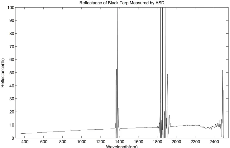
6.3 Measured reflectance of black uniform target . . . 65

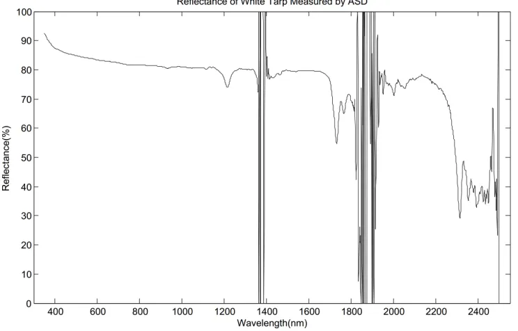
6.4 Measured reflectance of white uniform target . . . 66

6.5 Validation on white uniform target . . . 68

6.6 Validation difference ratio on white uniform target . . . 69

6.7 Validation on black uniform target . . . 70

6.8 Validation difference ratio on black uniform target . . . 71

6.9 Grass selection . . . 72

6.10 Validation on grass radiance . . . 73

6.11 Grass covariance matrix eigen values . . . 74

6.12 High resolution WASP imagery after color mapping . . . 75

6.13 Subpixel yellow plank spectra . . . 76

6.14 Subpixel target detection scene . . . 77

6.15 Compensated reflectance ROIs . . . 78

6.16 Subpixel yellow planks detection ROC . . . 80

6.17 Subpixel green planks detection ROC . . . 81

6.18 Divided scene image . . . 83

6.19 Subpixel green planks detection ROC in designed scene . . . . 84

6.20 Sensitivity of signal-to-noise ratio to sensor calibration error . 87 6.21 Sensitivity of detection to meteorological range . . . 88

6.22 Sensitivity of detection to relative calibration error . . . 89

6.23 Sensitivity of detection to false alarm rate . . . 90

(12)

Chapter 1

Introduction and Objectives

1.1

Introduction

System modeling is a quite helpful technique in understanding and

analysing system behaviour. A system could be modeled by characterizing,

analysing and then expressed analytically and mathematically. This kind of

model is an abstract description of the system which is being analysed. It is a

method to represent a real world system or a process analytically by low cost

calculation or software simulation. This kind of technique could be used in

many aspects to help understand the functionality of system. For example,

when we need to do an experiment, it would be very useful to analyse the

ex-periment first by breaking it down into several steps, and then estimating some

possible result in each step, qualitatively or even quantitatively. When doing

the experiment, people could get a general idea of how well the experiment is

conducted and finally how reliable the result is by comparing simulated and

experimental results. Or before a real system is built, some analytical work

could be done to validate the whole system design by theoretically modeling

the system, which is also helpful in characterising the real system. It is also

(13)

not be possible to build practically, or it is not necessary to build the real

sys-tem. In this case, system modeling is a key to analyse and study the system

effectively and efficiently.

In this thesis, the primary focus is on hyperspectral imaging system

modeling. Hyperspectral imaging is an imaging method collecting and

pro-cessing spectral information from a wide range across the electromagnetic

spectrum. A typical hyperspectral imaging system is illustrated in Fig. 1.1.

Our work focuses on system’s operating in the reflective portion of the optical

spectrum, extending from the visible part (0.4 to 0.7 um) to the Short-wave

Infrared (SWIR)(around 2.5 um). Hyperspectral sensors are made to

col-lect spectral radiance information in hundreds of narrow contiguous channels

typically 10nm wide. Most hyperspectral systems cover the visible and

near-infrared (VNIR)/SWIR bands, gathering radiance from materials based on

their reflectance information and incident radiation, and have proven useful

in various applications such as environmental monitoring [11], ground-cover

classification[2], mineral exploration [26], target detection [22] and subpixel

objection detection [23]. Hyperspectral imaging has advantages over regular

imaging since it expands regular image information from gray scale or RGB

into hundreds of spectral channels, which means even a single pixel contains a

feature vector with over 100 dimensions with an entire spectrum of reflectance

information. There is no need to acquire the prior knowledge of the sample,

(14)

to be collected. Hyperspectral imaging can also benefit from spatial

relation-ships between nearby spectral bands, which allows more accurate

[image:14.612.154.474.207.444.2]

spectral-spatial models for a better segmentation and classification of the image.

Figure 1.1: Typical hyperspectral imaging system[1]

A conceptual description of a hyperspectral remote sensing process is

shown in Fig 1.2, which shows an overall view of the whole system starting

from the power provided by the sun. The initial energy passes through the

atmosphere, getting partially absorbed and scattered in the atmosphere, and

then reflected by the corresponding landcover/target on the Earth’s surface.

After reflection, the light then passes through the atmosphere again before

(15)

be affected by atmospheric conditions such as solar angle, atmospheric model,

cloud, etc. At the instrument, light first passes through a set of lenses and

then reaches the detector. At the detector, the incoming energy is sampled

spatially and spectrally and then converted into an electrical signal. After

that, the signal is adjusted and digitized through the analog-digital converter

[image:15.612.156.461.275.506.2]

in order to be stored, analyzed and transmitted to a processing facility.

Figure 1.2: Remote sensing process[24]

At the processing stage, geometric registration and calibration might

be performed to make it possible to compare this data set with other data

sets. Feature extraction may also be conducted to reduce the dimensionality

(16)

in the image. At last, the data go through an interpretation stage depending

on different applications, which means for different needs there are different

processing methods to make full use of the data.

1.2

Objectives

From the description of remote sensing systems, there are at least three

major parts of the system: scene features, sensor characterization and

process-ing method. As a result, the system modelprocess-ing will be based on these three

respectively. The objectives of this dissertation are as follows:

• extend an existing analytical model for hyperspectral imaging system to

include a new instrument and new analysis scenarios;

• implement the analytical model in a new form which could be made

avail-able to the remote sensing community through an RIT-hosted website

to support hyperspectral imaging system design and parameter trade-off

research;

• validate the model by comparing with real world data collected from

RIT SHARE 2012 project both in full pixel target detection and

sub-pixel target detection scenarios, and investigate hyperspectral system

(17)

Chapter 2

Background and Related Work

In this chapter, an overview of background and related work in

imag-ing system modelimag-ing and its application is given. Several different example

imaging system models are described and discussed, including statistical data

based models and models that directly produce hyperspectral images.

2.1

Hyperspectral Imaging System Modeling Framework

The first systematic approach to analysze hyperspectral imaging system

was introduced in [21]. This paper serves as a cornerstone in the remote sensing

system modeling research based on input statistical data. In this paper, the

author explained the remote sensing system and several typical instruments

which cover the optical spectrum ranging from 0.4um to 2.4um. Then the

sys-tem and its working processes were separated into different unit blocks. The

surface reflectance statistics were assumed to be spectrally multivariate

Gaus-sian with a spatial correlation. The scene was spatially modeled as having

cells of diffuse reflectance (Lambertian assumption) with spatial correlation

from cell to cell. The solar and atmospheric model transferred the scene

(18)

is received by the sensor. Then the received radiance was mapped into sensor

bands according to a sensor channel response model. After reaching the sensor,

sensor noise sources were modeled by adding shot noise, thermal noise, etc, to

signal, with the noise being modeled as a zero mean random process. Each

noise source was assumed to be independent from each other and uncorrelated

from spectral band to spectral band. After noise was added, feature extraction

or selection might be performed to reduce dimensionality or to choose typical

bands. After all classes have been processed by the above system, an estimate

of the probability of error was made using a Bhattacharyya distance between

different classes. The modelled system was verified by existing experimental

results and shows consistency with real data.

The application model in the above paper was built for ground cover

classification. For different applications, there were different approaches to

system modeling to better simulate the scenario and complete the task. In

[35], the author presented a model for multispectral mine target detection.

Since the application was quite different, the Coastal Battlefield and

Recon-naissance Analysis (COBRA) multispectral sensor model was given in a more

detailed form, which was shown in Fig. 2.1. This system broke the whole

system into 4 main models. For the atmospheric part it used MODerate

res-olution atmospheric TRANsmission (MODTRAN) [3] as the model, and for

the detection model there was a mine detection algorithm committed to find a

(19)

application of data post-processing with the help of multi-spectral imaging

[image:19.612.119.514.184.449.2]

system modeling.

Figure 2.1: The COBRA multispectral sensor model [35]

Then in [15], the Forecasting and Analysis of Spectroradiometric

Sys-tem Performance (FASSP) model was first presented and then extended in [17]

to cover the full optical spectrum. A more clear and straightforward system

structure was introduced and the whole process was developed into separate

functional blocks, as shown in Fig. 2.2 . This updated version of system model

now could take multiple background classes, which were described by their first

(20)

these statistics become the scene model. It used MODTRAN for atmospheric

effects, which was similar with previous research. The sensor model was also

like the original modeling in [21] except it was extended to the HYDICE

in-strument [32] with a broader wavelength range. The FASSP model has been

validated in a number of scene types with real world data by comparing how

[image:20.612.127.498.282.498.2]

different parameters affect the performance of detection.

Figure 2.2: FASSP model framework [16]

2.2

Hyperspectral Imaging System Modeling

Improve-ments

After the main skeleton for hyperspectral imaging system modeling was

(21)

In [19] the background model was simply a linear combination of different

background class spectral statistics, and [20] improved the linear model to

include elliptically contoured multivariate t-distributions to better depict

em-pirically observed backgrounds, which lead the system model to make more

realistic performance predictions without describing a complex scene.

For the atmospheric effect modeling, LOWTRAN or MODTRAN has

been used to convert reflectance statistics into radiance data based on

at-mospheric parameters, and this has been recognized as the most correct and

accurate way to simulate the process. As a result, improvement in this part

was rarely seen.

Improved versions of the FASSP model have kept the framework of the

sensor model similar, but took the mean and covariance of the input signal

and then applies sensor effects such as sensor spectral response, sensor noise

from different sources, etc. The improvement in the sensor modeling could be

extending the sensor type of different wavelength bands, different sensor

re-sponses and different noise models. [17] enhanced the sensor model to include

a dispersive spectrometer model and a Fourier transform spectrometer model.

There were sensors focusing on different wavelength bands. For example for a

certain type of LWIR sensor, excess low-frequency noise (ELFN) was

signifi-cant in forming the noise. As a result, the noise model needed to be improved

to better simulate the sensor.

(22)

the sensor to include polarimetric features. In [24], polarimetric features were

added into the sensor, which increased the information dimensionality. As a

result, the system performance could be increased by using the new

informa-tion, and also this polarimetric model has made the hyperspectral imaging

system modeling more complete.

Different applications have different algorithms, and another difference

in system modeling lies in the processing of the data. There were different

data processing algorithms implemented for different applications. For

sup-porting relatively small target detection and high sensor altitude imaging, [15]

extended the application into subpixel target detection, based on a subpixel

object model using the subpixel fraction to define the fractional area of the

pixel occupied by the object within direct sight of the sensor. In the subpixel

target detection scenario, several pairs of parameter trade-offs, and also in

different combination of backgrounds were discussed and analyzed to better

understanding the detection performance. [14] used the system model to

pre-dict unmixing performance, which included a different post-processing method

applied to the data. Then the data observed from real world was shown to

compare well with the predicted result, which validated another application of

the FASSP model.

For the above applications and modeling, an assumption that the data

collected have been perfectly geometricly corrected is made. In [9], the author

(23)

ge-ometric registration, and gave an in-depth simulation of EnMAP acquisition

geometry.

The models discussed above are all statistical data based, which means

the input and output are some statistics of the data, such as mean and

co-variance. This modeling method may not be very intuitive, but it reduces the

computational cost and sometimes reduces the unnecessary system complexity

for specific applications.

Besides the theoretical models discussed above, the Digital Imaging and

Remote Sensing Image Generation (DIRSIG) tool deserves mention as a

com-plex synthetic image generation application being used by the remote sensing

community. It is a popular system modeling tool being widely used among the

researchers in this field [37]. It produces simulated multispectral or

hyperspec-tral remote sensing images by calculating the sensor reaching radiance, and it

also produces predicted image pixel by pixel, not just some statistical data.

This feature encourages many algorithm developers to use DIRSIG to validate

their algorithms with the help of pixel level ground truth images. Compared

with the FASSP model mentioned above, DIRSIG is a more comprehensive

model to simulate the sensor reaching radiance at the pixel level, and since it

can do pixel level prediction, the computational cost is huge for hyperspectral

imaging systems. Also, it needs more complex scene definition, including the

3D model and BRDF for different objects in the scene. Second, since it does

(24)

simu-lated data first then apply further processing in another platform. However,

FASSP includes the post processing for the data and also the algorithm

evalu-ation metric to easily estimate the system performance under some proposed

conditions. Third, the DIRSIG tool has put some restrictions on users and

DIRSIG training is required before using, and it is better to have a model

open to public and ready to be used easily.

2.3

Summary

An overview of the background of imaging system modeling was

dis-cussed and the related works in this area were given. Different examples of

statistical data based imaging system models were provided and the

improv-ing from different system aspect was discussed. Then DIRSIG was introduced

as a more comprehensive model and a popular tool among researchers in the

remote sensing community. By comparing DIRSIG with the FASSP model,

the advantages and disadvantages were discussed, and we now see that an easy

to use and easy to access system modeling tool is in need by remote sensing

(25)

Chapter 3

End-to-End Hyperspectral Imaging System

Modeling

This chapter introduces hyperspectral imaging system modeling mostly

by reviewing literature [16] [34] and some extended discussion. The

end-to-end hyperspectral imaging system involves all the components in the scene,

including illumination, surface reflection, atmospheric effects, the sensor,

in-cluding spatial, spectral, thermal and radiometric effects, and the processing

algorithms, including calibration, feature selection, and application algorithm

to complete the whole process [17]. The main assumption this modeling

ap-proach is based on is that the various surface classes could be characterized

by their first and second order spectral statistics. Then all the effects could

be modeled as transforms and functions to these statistics. Based on this

fundamental assumption, these three major functional blocks – scene, sensor,

processing – will be discussed below respectively.

3.1

Scene Model

In a remote sensing system, the primary source of flux incident on a

(26)

sources, which are reflected, scattered, etc, then detected by sensing

instru-ment. Fig. 3.1 shows the main atmospheric effects on the flux and several

[image:26.612.132.505.216.491.2]

major incoming flux paths to the sensor.

Figure 3.1: Solar and atmospheric effects [24]

There are three different radiances described in Fig. 3.1. Radiance A

passes through the atmosphere directly. It is then reflected by the reflector,

which may be defined as target or background in a target detection scenario,

and then bounces back to the atmosphere before finally reaching the sensor.

(27)

reflected back to sensor. This radiance is called downwelled radiance. Radiance

C is the solar irradiance scattered from the atmosphere then directly into

the sensor without arriving at the reflector on earth. This radiance is called

upwelled radiance or path radiance. Also, there are other kinds of radiance

reaching the sensor such as the adjacency effect which is sun light reflected

from an adjacent surface, background radiation, and then scattered by the

atmosphere into the sensor. The adjacency effect is captured in the model by

using the overall average surface scene reflectance in the whole scene.

Figure 3.2: Light reflection geometry [34]

To describe the radiance propagation process, the geometry of a basic

light reflectance scenario is presented in Fig. 3.2. The optical property of a

surface reflection is usually described by the bidirectional reflectance

(28)

directions [27]. It is defined as the ratio of the radiance scattered into the

direction described by the orientation angles (θr, φr) to incident irradiance

from (θi, φi), i.e.

f = L(θr, φr)

E(θi, φi)

[sr−1] (3.1)

This is the general form of BRDF, and the ratio varies for different reflecting

directions. However, in most cases the reflection surface is considered as a

perfect Lambertian radiator, which means the reflection has the same radiance

in all directions. Feng et al. in [6] show the reflectance factor (rrF) is related

to the bidirectional reflectance (rBRDF) by a simple factor ofπ steradians, i.e.,

rBRDF[sr−1] =

rrF

π[sr] (3.2)

Then the complicated directional related coefficient could be simplified into a

simple surface reflectance factor. Then the radiance A reaching the sensor is

expressed as:

Lr =

τ cosθiEsrrF(λ)

π [W m

−2

sr−1µm−1] (3.3)

whereLr is the direct solar reflected radiance, τ is the surface-to-sensor path

transmittance, θi is the incident angle, Es is the solar spectral irradiance on

the surface from its direct transmission through the atmosphere andrrF is the

reflectance of the surface according to different wavelength.

Radiance B is the downwelled radiance reflection. It comes from the

photons incident on the reflecting surface due to the solar scattering from the

(29)

is introduced, and it describes the spectrally related angular scattering

coef-ficient for the composite atmosphere, where λ is the wavelength, and σv is

the angle between the incident flux and the flux to the surface. The scenario

is modeled as the radiance is scattered by small volume elements of the

at-mosphere then reaching the target, which means to integrate all radiances

from ”small volume elements” onto the target. Then the radiance reaching

the target from direction zenith angleθd and the azimuthal angleφd could be

expressed as:

Ldi(θd, φd) =Esλ0 Z

τL1(λ)τL2(λ)βsca(λ, σv)dr (3.4)

whereE_sλ0 is the exoatmospheric spectral irradiance, τL1(λ) τL2(λ) are the

L-path transmission values, and r is the length of volume-target path. Then

based on the Lambertian surface assumption, the surface reflected downwelled

radiance originated from direction zenith angleθd and the azimuthal angle φd

could be considered as:

Ld=

τR LdicosθdrrF(λ)dΩ

π (3.5)

wheredΩ = sinθddθddφd and τ is the surface-to-sensor path transmittance.

Radiance C is the upwelled radiance, which has not been reflected, just

scattered by the atmosphere before reaching the sensor. From the derivation

of the downwelled radiance case, this case can be considered similar to the

(30)

expressed as:

Lu(θd, φd) =Esλ0 Z

τL1(λ)τL2(λ)βsca(λ, σv)dr (3.6)

whereτL1(λ)τL2(λ) are the L-path transmission values from sun to scattering

atmosphere volume to sensor in this case.

In practical research and application, the solar irradiance, downwelled

and upwelled radiance are often estimated using an atmospheric scattering

model, like MODTRAN. Except for these three major energy paths, there are

also other energy paths like thermal radiance which could also be computed

by MODTRAN. In our model, MODTRAN is called several times to turn the

reflectance statistics into radiance statistics according to the atmospheric

con-ditions. The output data of MODTRAN includes different columns to describe

each path or source of the radiance varing among a range of wavenumber. For

example, the GRND RFLT column is the total ground reflected radiance,

which is the sum of Lr and Ld, SING SCAT column is the single-scattered

radiance term of the path radiance, and SOL SCAT column represents the

multiple-scattered radiance term of the path radiance. But actually the path

radiance includes not only these terms, and to make it more accurate, a

MOD-TRAN run that the target surface reflectance is set to 0 is included, and then

the GRND RFLT will be 0. As a result, TOTAL RAD becomes the rest part of

total radiance except for reflected radiance, which means it’s the path radiance

we are looking for, Lu, described by Eq. (3.7).1 In each call, the Lr, Ld, and

(31)

Lu are extracted from corresponding columns, and also the thermal radiance

from a specific column is extracted, then combined into corresponding totalL

in each scenario.

In our model, the scenario is for subpixel target detection in multiple

backgrounds [16]. For background class modeling, each background class m

calls MODTRAN respectively, and another MODTRAN call is made for the

average background scene. Then the total mean radianceLb for each class is:

Lbm =LS(ρm) +LP(ρave)

Lbave =LS(ρave) +LP(ρave)

(3.7)

where the LS is the total ground reflectance radiance corresponding to the

GRND RFLT column in MODTRAN output data for each background class,

LP is the average background path radiance term, ρm is the mean reflectance

statistics for classm, and ρave is the scene average reflectance, which is

calcu-lated by the scene fractions fm in Eq.(3.8):

ρave = M X

m=1

fmρm (3.8)

MODTRAN runs not only using the reflectance data, but many other

parameters, such as the solar angle, sensor altitude, atmospheric model, etc.

In our model, most of them can be specified by the user, which allows the user

to have a more flexible model to use, but also the system provides a set of

(32)

default values and detailed hints for each parameter to make it more friendly

and easy use.

Contrary to the atmospheric parameters, the mean and covariance

spec-tral reflectance statistical data for surface background and target classes are

obtained prior to the modeling. They may come from some database which

includes measurement samples for different surfaces or from direct

measure-ment for some specific surfaces or targets. The measuremeasure-ment is done by a

spectroradiometer, and after obtaining multiple samples of the hyper

dimen-sional reflectance vector, the reflectance mean of the surface is obtained and

the reflectance covariance matrix could be calculated.

For target class, the radiance propagation is similar, and the mean

spectral radiance for target in open is calculated as in Eq.(3.9)

˜

LT =LS( ˜ρT) +LP(ρave) (3.9)

Due to a subpixel scenario, the ˜ρT is actually a weighted sum of the target

mean reflectance and the background classm∗ it is in, as in Eq.(3.10):

˜

ρT =fTρT + (1−fT)ρm∗ (3.10)

where fT is the subpixel fraction of the target takes in a pixel, with a range

between 0 and 1. The rest of the pixel is the background class, which accounts

for the second term in the equation. This equation merges the target and

(33)

transforms this subpixel target detection problem into a regular target

detec-tion problem. This pixel could be considered as the new full pixel target and

then the total estimated target radiance is based on the weighted sum of the

pixel reflection statistics, which is the new pixel size target.

The radiance mean statistics calculation is discussed above, and the

radiance covariance transform from reflectance to radiance follows similar

lin-ear atmospheric model assumed in the above radiance mean calculations. The

main concept in the calculation is a linear interpolation of spectral radiances

calculated for surface albedos from zero to one according to the entries in the

reflectance covariance matrices. This calculation makes use of several diagonal

matrices: ΛLS1 is the total surface reflected radiance for surface reflectance 1,

ΛLP1 is the path scattered radiance for surface reflectance 1, and ΛLP0 is the

path scattered radiance for surface reflectance 0. Then the spectral radiance

covariance matrice for background class m, ΣLBm, and average, ΣLBave, are

expressed as:

ΣLBm = ΛLS1gBΣρBmΛLS1+ [ΛLP1−ΛLP0]gBΣρBave[ΛLP1−ΛLP0]

ΣLBave = ΛLS1gBΣρBaveΛLS1+ [ΛLP1−ΛLP0]gBΣρBave[ΛLP1−ΛLP0]

(3.11)

where ΣρBm, ΣρBave are the corresponding reflectance covariance matrices for

each background class, average background class, and gB is the background

class reflectance covariance gain factor specified by the user.

For the target class, the situation becomes a little more complicated. It

(34)

ΛLS1 , then the total target radiance covariance matrix is expressed as:

ΣLT =fT2ΛLS1gTΣρTΛLS1+ (1−fT)2ΛLS1gBΣρBm∗ΛLS1+

[ΛLP1−ΛLP0]gBΣρBave[ΛLP1−ΛLP0]

(3.12)

where gT, like gB, is the user specified scalar for the target reflectance

co-variance matrix and ΣρBm∗ is the reflectance covariance matrix for class m in

which the target resides in.

At this point, the transformation from reflectance mean and covariance

statistics into radiance mean and covariance based on the scene parameters is

finished, which means the radiance reaching the sensor is obtained.

3.2

Sensor Model

The sensor model takes in the spectral radiance mean and covariance

statistics of the backgrounds and target, applies sensor effects, such as noise

effects, channel response, caliberation, etc, to the radiance statistics and then

outputs the processed data to simulate the process that an image is taken by

the hyperspectral instrument for further processing.

There are different kinds of sensors having different working spectral

bands, channel responses, resolutions, noise features, etc, which requires our

model to be built in a generalized form and allow different specifications for

different sensors.

The input data (mean vector and covariance matrix) is usually

(35)

samplings at specific wavelengths with an equal margin or a distribution over

a section of spectral band. As a result, the spectral band and samples at

specific wavelengths of input data should be mapped into the set of spectral

bands and wavelengths specified in the sensor specification file to comply with

the sensor working condition. Actually, in order to speed up the calculations,

this mapping is done before the reflectance mean and covariance statistics are

used in the scene model. After the background and target classes as well as

the sensor are specified at the beginning of this model, the reflectance mean

vectors and covariance matrices are interpolated into the wavelengths

accord-ing to the sensor specification, and then the reflectances at these wavelengths

are recorded in the MODTRAN reflectance specification file for its running,

which provides a more accurate output from MODTRAN at and around these

wavelengths.

Usually, MODTRAN has a much finer spectral resolution output than

the resolution of sensor, and at this step, the modeling could be considered

as the sensor takes samplings at its descrete wavelengths from the much finer

MODTRAN sequence output. Each sensor wavelength needs a channel

re-sponse function to describe how the sampling works. In this model, the

chan-nel response function is modeled as Gaussian distributions with a center of

the specific wavelength and width of±3 times the standard deviation, which

is defined by the channel bandwidth. As a result, each response output for

(36)

around that wavelength.

After the channel response modeling, some major noise sources, such

as the detector noise, calibration noise, analog-to-digital converting noise, etc,

are modeled. The sensing instrument works like a hyperspectral camera, and

the whole working process is described in Fig.3.3. Generally speaking, there

Figure 3.3: Sensor working model [24]

are different types of noise at different stages of the sensor pipeline. For the

detector related noise, there is photon noise, which is related to the input

sig-nal level, and thermal noise and readout noise, which are non-related to the

input signal. After the detector during the calibration, there is percentage

calibration error. Then at the quantization and data link level, there is analog

to digital noise and the bit error in the communication link or recording

chan-nel. Then the noise process is modeled by adding variances onto the diagonal

entries of the input covariance matrix, which means the modeled noises are

all independent on their own channel, and assuming there is no inter-channel

noise correlation.

(37)

input radiance is transformed into electrons by Eq.(3.13) [18]. The number of

photons emitted and detected in a specific time span could be modeled with a

Poisson distribution. If a random variable follows such a distribution, then it

will have the same mathematical expected value and variance. As a result, if a

sensor is receiving 40000 photons per time interval, which could be considered

as the expected value, then the standard deviation error due to photon noise

would be √40000 = 200 photons.

σnp = p

L×Od×AΩ×τ×η×t×∆λ×CU ×λ/(h×c) (3.13)

where

L: input spectral radiance [mW cm−2srµm];

Od: radiance channel degradation coefficient;

AΩ: system throughput [cm2sr];

τ: optical transmittance;

η: quantum efficiency;

t: integration time [sec];

∆λ: spectral channel bandwidth [µm];

λ: spectral channel central wavelength [µm];

(38)

Except for the system throughput, the parameters above are included in

most sensor specifications. But the sensor aperture size d and instantaneous

field of view θif ov are provided to compute the system throughput by Eq.

(3.14).

A=π(d/2)2

Ω =4πsin2(θif ov/4)

(3.14)

The thermal noise and readout noise are always considered as a property of

sensor and given in the sensor specification file together as fixed noise. It

is also possible to obtain them by conducting an experiment specifically for

measuring them. The total noise at the detector is the squared sum of the

three according to the variance calculation method, and since the fixed noise

includes thermal noise and readout noise, then the total noise variance at the

detector could be expressed by Eq. (3.15), where σnf is the fixed noise in

electrons.

σ_nd2 =σ2_np+σ_nf2 (3.15)

Then the obtained detector noise needs to be converted back into radiance

σLdn, and a user specified detector noise gain factor gdn is applied on it. After

this, the scaled detector noise is added onto the diagonal elements of the class

m covariance matrix, as shown in Eq.(3.16) for each channel i

Σdn_m(i, i) = Σm(i, i) +gdn2 σ 2

Ldn(i) (3.16)

Second, another noise source is the relative calibration noise CR. For

(39)

channels with a percentage describing the relative fluctuation centering on the

mean input signal level Lm(i) like a standard deviation in each channel. For

channel i and class m, this noise modeled as a variance adding onto signal

covariance matrix is as shown in Eq.(3.17)

Σdn_m+c(i, i) = Σdn_m(i, i) + [Lm(i)×(CR/100)]2 (3.17)

Third, analog-to-digital quantization process in the pipeline results in

quantization noise, and the bit error noise is from the data communication

link or recording system. Both of these noises are functions of the sensor

radiometric resolution, and in our model the sensor resolution is the least

significant bit (LSB) in the sensor specification file. According to some basic

statistical knowledge on variance of a uniform distribution, the quantization

noiseσ2

nq can be expressed as:

σ2_nq =LSB2/12 (3.18)

whereLSB has a units of electrons.

For the bit error noise in the data communication or recording process,

our model assumes that the bit errors are uniform in the whole data which

means for N bits data package, the bit error rate for each digit is the same

and there is no source or channel coding on the data which means the data is

modeled as binary data stream. If the error bit is at a higher digit, the error

(40)

usually quite low compared with other noises, multiple bit errors happening

at the sameN bits data package has a much lower probability and as a result

only one digit error is considered without taking the case of multiple bit errors

in one package into consideration. Then the bit error noise is considered as an

average data error of error bit on each digit, and expressed in Eq.(3.19):

σ_nB2 _e = Be

N

N−1 X

n=0

(2nLSB)2 = LSB

2_B

e

3N 2

2N ₋₁

(3.19)

Then the σ2

nq and σnB2 e will be converted back to radiances to add onto the

signal matrix diagonal elements to complete the whole sensor noise model

process.

In the sensor process, another important parameter to characterize the

sensor performance is the signal-noise-ratio (SNR), which is independent for

each different class. The ”signal” is the input mean radiance vector for each

class and the ”noise” is the square root of the sum of several noise terms

calculated above in the form of standard deviation. For class m (target or

some background), the SNR is expressed as:

SNRm =

Sm q

σ2

nd+σC2R +σ 2

nq+σ2nBe

(3.20)

After the sensor model, the radiance mean and covariance statistic data

(41)

3.3

Processing Model

If the data processing module is considered as a black box, the

in-strument output radiance data obtained above will be the module input, the

internal control mechanism will be determined by the application required,

such as target detection, tracking, unmixing, etc, and then the output of the

black box should be some metric to characterize the performance of the

ap-plication based on some specific criterion designed for that apap-plication. Since

this paper is focusing on the scenario of subpixel target detection, then the

process and metrics for target detection will be used, such as the feature

se-lection/extraction as the data pre-processing method, and probability of

de-tection vs false alarm rate as the evaluation metric.

For target detection or even other applications, the data used in the

processing algorithm of a hyperspectral system is usually not the radiance

col-lected by the instrument directly, because the radiance data includes the effect

of the atmosphere which loses universality for the same target but in different

atmospheric conditions. And as a result, the collected radiance data needs to

be transformed into some atmospheric independent form which is usually the

surface reflectance, and this process is called atmospheric compensation.

There are different atmospheric compensation methods to retrieve the

surface reflectance. Generally there are two types of methods: one has the

ground truth data when it is possible to put some pre-known reflectance panels

(42)

in-scene method and just uses the in-scene radiance information collected when it is

difficult or impossible to obtain good ground truth information. The ground

truth method, a.k.a. empirical line method (ELM) [36] is widely used in

different conditions and it assumes the reflectance and the radiance collected

are linear with each other and they should fit in a line. Then the ground

truth information could be used to compensate for the atmospheric effects

and compute the target reflectance. For in-scene methods, the most common

and simple one is called darkest pixel (DP) atmospheric compensation method

[29]. Since the radiance reaching the sensor could be expressed asL=Crt+Lu,

whereC is a constant relevant to solar irradiance, atmosphere transmittance,

etc., rtis the target reflectance, and Lu is the upwelled radiance. This method

assumes that the minimum scene radiance is the upwelled radiance when the

target has a zero reflectance. The constant C could be obtained by the scene

color standard approach [30] and then the reflectance could be computed.

In this model, the ELM method is used for atmospheric compensation

by using low and high reflectance panels, in our case 0.1 and 0.6, to compute

the offsetb and slopek of the linear relationship between the radiance and the

reflectance. The choice of 0.1 and 0.6 rather than 0 or 1 is for excluding the

nonlinearity and noise present close to 0 and 1. Then the mean reflectance

is obtained by finding the corresponding mean radiance for each channel

ac-cording to the fitted ground truth line. For the radiance covariance matrix, to

(43)

matrix has been built to multiply its element with the corresponding element

in the same row and column from the covariance matrix, and the offset b is

not applied since covariance does not take offset in the calculation.

After the estimated reflectance mean and covariance data are obtained,

the next step is the feature extraction due to the high dimensionality of the

original data, which is always hundreds of channels for hyperspectral image.

There are many different ways to extract the features from the obtained

multi-dimensional reflectance data. One easy and simple way is just to choose the

reflectance data from preset bands in spectrum such as visible region, VNIR,

SWIR, etc, or a selection of channels from different spectral regions to avoid the

effects of atmosphere and water absorption. Besides this, principal component

analysis (PCA) is also a widely used to process the hyper-dimensional data to

reduce the dimensionality, and there are modified version of PCA according to

correlation between channels [39] or based on wavelet decomposition [8]. There

are also other methods to perform the dimensionality reduction according to

or designed for different applications, but the idea is also to apply a linear

transform, which is described by a transform matrix Ψ, on the mean vector

and covariance matrix, like what is showed in Eq. (3.21):

Fm =ΨXm

ΣF m =ΨΣXmΨT

(3.21)

whereXm means the input mean reflectance vector of class m(target or

(44)

have similar meaning but they are matrices. The transform matrix Ψ is a m

byn matrix, where m is the dimension of feature space and n is the original

mean vector length. This transform matrix reduces the data dimension fromn

tom. In our model, the feature selection implemented is the channel selection

method, which allows the users to select multiple or all channels from the band

range of the sensor they have chosen.

After the feature extraction, the projected data could be used to

per-form the application in a given scenario: subpixel target detection in our case,

and then a designed performance metric will be adopted to evaluate the system

performance.

There are different cases for target detection: one is the target is

un-known, which means the target spectral feature is unknown and the other is

that the target spectral character is known. In our case, since the target mean

reflectance vector and covariance matrix are already known, so the latter case

will be discussed. The most common target detection algorithm for a set of

sampling based data is the spectral matched filter (SMF) when the target

is known. The concept of matched filter was first introduced by the radar

signal detection community when they were looking for an optimal filter to

detect the signal by maximizing the signal to noise ratio (SNR) in additive

white Gaussian noise [28]. In the case of remote sensing, the method has been

expanded to deal with a multi-dimensional signal, the hyperspectral image,

(45)

However, in remote sensing, the ”noise” is not additive stochastic noise any

more but the scene variation. The scene variation is included into the system

by the surface reflectance measurement, and the data measurement process

could be considered as a sampling process. According to the central limit

theorem the sampled surface reflectance data follows a Gaussian distribution

when the number of samples is considered large enough. The scene variation

has similar feature as the ”noise” in the radar signal detection matched filter,

and the SMF should be also work for hyperspectral target detection [33].

The SMF is considered as a two-step process: the first step is to project

the background average and target reflectance mean vector into a normalized

space using the background covariance matrix, which makes the sample points

distribute uniformly around the origin in the ”multi-dimensional sphere”; the

second step is to project the normalized background average vector onto the

normalized target vector. After the two-step process, a threshold will be

ap-plied to make a decision to balance the false alarm rate and detection rate.

This whole process could be expressed as:

SM F(ρ_bF T) =[Σ −1

2

ρF Bave(ρbF T −ρbF Bave)] T_Σ

−1

2

ρF Bave(ρF T −ρbF Bave)

=(ρ_bF T −ρbF Bave) T

Σ−_{ρF Bave}1 (ρF T −ρbF Bave)

≥η→target

<η →non−target

(46)

Figure 3.4: SMF for a simplified 2-D scenario

Fig. 3.4. shows a general idea of how this two-step method works

when the multi-dimensional target detection problem is simplified into a 2-D

problem.

In many cases, it is helpful to scale the result of matched filter to one in

the direction of target feature vector, and it could be completed by normalizing

(47)

is called constrained energy minimization (CEM) [5], and it uses the target

feature vector and estimated background information to minimize the energy

from the background and at the same time normalize the result to one if the

sample feature vector matches the target feature vector, which is expressed in

Eq. (3.23)

CEM(ρ_bF T) =

(ρF T −ρbF Bave) T_Σ−1

ρF Bave(ρbF T −ρbF Bave)

(3.23)

From Eq. (3.23) we can see, if ρ_bF T = ρF T, the result will be normalized to

1. In order to simplify the calculation, operator w has been introduced into

our expression, and it is the projection vector to be applied on the translated

sample vector. In fact, this operator is just a part of the whole expression of

CEM equation and it is expressed as follows:

w= (ρF T −ρbF Bave)

T_Σ−1 ρF Bave

(3.24)

ThenCEM(ρ_bF T) becomes:

CEM(ρ_bF T) = w(ρbF T −ρbF Bave) (3.25)

In our model, the operator w is used to transform the estimated reflectance

vectors into theCEM projected space with meanθ and varianceσ2in order to

calculate the false alarm rate and detection probability to evaluate the target

detection performance. In the calculation of σ2

T and σBm2 , since w and ρbF Bave

are fixed, and then wρ_bF Bave is considered as a constant scalar to be ignored

(48)

cov(wρ_bF T). According to the properties of covariance calculation, cov(wρbF T)

equals towcov(ρ_bF T)wT Then the following equations show the results:

θT =w(ρbF T −ρbF Bave) (3.26)

θBm =w(ρbF Bm−ρbF Bave) (3.27)

σ_T2 =wΣb_{ρF T}wT (3.28)

σ_Bm2 =wΣbρBmwT (3.29)

where m is the background class index for all backgrounds, ΣbρF T and ΣbρF Bm

are the estimated target and background class reflectance covariance matrices

using ELM based on corresponding radiance matrices [18].

After these parameters are obtained, the probability of detection PD

and false alarm rate PF A can be calculated. According to the central limit

theorem, the mean and variance parameters of feature space background and

target statistics obtained by operator w generally follow a Gaussian

distribu-tion, and based on this assumpdistribu-tion, Fig. 3.5 shows a simplified description of

relationship among PD,PF A, and threshold variable x.

In our model, there are not only one background class, which means

the situation is more complicated for PF A and PD than the one background

scenario. PD should be a combination of PDm which is computed for each

different background class m based on PF A values. Since finally receiver

op-erating characteristic curve will be used to evaluate the system performance

(49)

Figure 3.5: Concept of one background target detection by thresholding

threhold array to calculate differentPF A and PD will have large error in small

PF A region. As a result, a PF A array is used to calculate threshold x, then

calculating the actual PD and PF A based on the fraction of background and

their corresponding PDm.

Since the Gaussian distribution assumption is adopted, then the

thresh-oldxmfor achievingPF Ain classm, and correspondingPDmshould be obtained

by:

xm =θBm+σBmΦ−1(PF A) (3.30)

PDm =

1 √ 2π Z ∞ xm exp

−(x−θT)

2

2σ2 T

dx= 1 2

1−erf(x√m−θT

2σT

)

(3.31)

where Φ−1_{() is the inverse of cumulative distribution function (CDF) and erf}

is the error function. There is aPDm for each of different background classm,

and according to the barrel theory, the minimum PDm is the system PD and

(50)

the updated PF A as a weight combination of PF Am for different background

classes according to their fraction in scene [18]. These could be expressed as:

PD =minPDm (3.32)

PF A = M X

m=1

fmPF Am(x∗m) (3.33)

Then after all PD and updated PF A are obtained according to each element

in preset PF A array, the ROC curve can be plotted, and the subpixel target

detection system performance finally can be evaluated.

3.4

Summary

In this chapter, the detailed system modeling approach is introduced.

The whole imaging system model has been separated into three major parts:

scene model, sensor model and processing model. The scene model mainly

deals with the solar illumination, atmospheric transmittance and surface

re-flection, and the transform between radiance and reflectance during the

pro-cess; the sensor model includes the sensor response function simulation and

the sensor noise modeling to add onto the radiance signal obtained from the

scene model; the processing model has two parts: one is the feature selection

as the pre-processing, and the other is the processing algorithm and algorithm

evaluation metric depending on the specific application in the process, which

is subpixel target detection in this case. In this stage, the target detection

per-formance is evaluated by the traditional PD, PF a method for the ROC curve

(51)

Chapter 4

Model Implementation

Based on the analytical model described above, the end-to-end model

is implemented and made available to the hyperspectral imaging research

com-munity through an RIT-CIS website working as a web application. It allows

the user to select different sensors, targets and backgrounds for system

model-ing or choose some pre-defined scenarios with fixed settmodel-ings. Also, for different

parts in the model, the user can also adjust some parameters to meet their

specific needs, including the scene, sensor, and target parameters. The

end-to-end modeling system is divided into two parts in the implementation: the

front end, which is the user interface providing an interaction with the

sys-tem parameters; and the back end, which is the algorithm computational core

doing all the calculation and data recording.

4.1

System Workflow

The system depends on a Python website framework, one kernel

ex-ecutable file and corresponding configuration files. Before the system runs,

the configuration file ”pathconfig.ini” should be set up first. It defines the

(52)

H

yp

er

sp

ec

tr

al

Im

ag

ing

S

y

st

em

P

re

d

ic

ti

on

M

od

el

/s ta rt p age /c u st o m ize /e rr or /p ar a se le ct ion /r es u lt C la ss s ta rt p a ge C la ss p ara C la ss c u st o m ize C la ss r es u lt e x ec u ta b le f il e “ m a in ” P u ll p ar a me te rs fro m c or re spon d ing d es c ri p ti on f ile M o d T ran p at h conf ig .i ni u ser C u st o m iz ing? “ m a in ” g o e s w rong? Us e rs s el ec t se n sor , ta rg e t, b a ckgr o und Us e rs m ak e c h a n g e s to p ar a m e te rs U se rs r edr aw p lo ts pr e-f il l te x t b lo c ks In it ia li ze s e le ct ab les W e b p y f ra m e w ork F R O N T E ND B AC K E ND H T ML J ava S c ri pt C SS P yt h on C ++ Y N N Y R ad ia n ce

SNR ROC

(53)

data file folders and other configuration parameters. The path to this file is

pre-defined in the C++ code. The item sequence should not be altered in this

file to ensure successful access. The pfile includes most system parameters and

there are different pfiles for different predefined scenarios and user specified

conditions. C++ code will use current pfile corresponding paths to proceed.

The executable program requires pathconfig.ini file to run and outputs 4 data

files as result for plotting and user downloading.

From the startpage, pfile selection choices are predefined in the form

configuration. Each choice is corresponding to a specific pfile (.fcm file), which

specifies most parameters of the scene, target, background and sensor. Fig.4.2

shows the predefined scenarios and user customized scenario for choosing on

the startpage.

Figure 4.2: Scenario selection

(54)

page will be rendered and parameters will be filled into the parameter

adjust-ment page according to the selected pfile.

If the user customize option is selected, a customization page will be

initialized and rendered. This customization page includes different sensor,

target and background choices for user to choose. If the user submits without

choosing any background, an alert will popup. Users can use ”ctrl” or ”shift” to

do multiple background choices. If the submit is successful, the parameters and

corresponding wavelength choices will be passed over to the render parameter

adjustment page, with default prefilled values.

Then the paraselection HTML page is reached. Users can specify those

parameters by adjusting them or just run with default values. Then the

pa-rameters from the form will be used to generate a file, and this parameter file

will be passed to the C++ executable file for main calculation. If the

param-eters are legal inputs, and the user has selected some of the wavelengths to

proceed, the result will be obtained after ”submit”.

If nothing is wrong, the result page could be reached and a folder named

by the user’s cookie is created to store the output data. The output data is

stored as text files on the server for further investigation such as plotting

different curves. They also can be downloaded by users. Also, the parameter

file used for the executable file is stored for user review. If a user runs the

model for multiple times in the same session, the new results will overwrite

(55)

retrieval. Fig.4.1 shows the workflow of the system. However, if there were

some internal errors occurred during the running, the error page is returned

and the user will be redirected to the startpage to start over.

During the whole website visiting and working process, there is only

one file between the front end and back end as described in the flowchart of

Fig. 4.1: code.py. In this code, one part provides support for url mapping and

the other part for form generation. For each different class, the web page will

call corresponding class to complete its own task.

4.2

Front End

Here the ”front end” mainly means the user interface, including the

forms, interactive web pages and displayed feedback. The whole website

struc-ture is based on the Python Webpy framework, and the web pages are mostly

written in HTML, JavaScript and some CSS.

Webpy is a very simple and straightforward website solution using a

Python framework. There is only one Python source code file controlling

the whole website including the appearance and content, and also interacting

with the back end data retrieval and functions. Fig.4.3 shows the sensor,

background and target selection user interface. According to the selection of

this page, the corresponding background, target and sensor information will

be recorded to initialize the prefilled values in the forms of the next page. It is

(56)

Figure 4.3: Sensor, background and target selection

forms which are defined as form blocks, and the details of these form blocks

could be initialized with prefilled values by generating the required HTML

code in corresponding Python functions. Fig.4.4 shows the parameter selection

interface. The prefilled values in parameter selection forms are dynamically

generated based on the sensor, background and target selections.

Each different web page in this framework matches a class (or function)

in the main code file, and each page contains a form submit system. In each

(57)

(58)

Figure 4.5: Security check example

on that page and there also is a security check. The one to one match between

(59)

Referring to the security check, not all work is done by Python at the

server side. Following the general design process of web pages, the security

checks are mostly accomplished by Javascript at the user’s end to give instant

feedback and reduce the unnecessary server cost. In our model, the security

check is performed to ensure that the data format and value upper and lower

bounds chosen are valid and to provide warning and suggestions when they

are not. For example, if the user forgot to choose wavelengths for the feature

selection, then a warning will pop up and the corresponding area will change

background color to notify user, as shown in Fig.4.5. Then the user needs to

do corresponding corrections to make the system run. Fig.4.6 shows part of

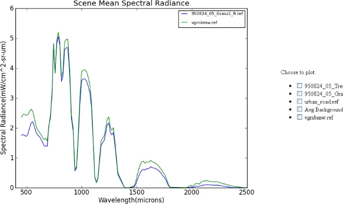
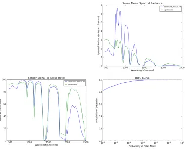
the prediction results. Users can choose the classes on the right to replot the

curve, or download the corresponding data file to plot or analyze using other

software.

4.3

Back End

At the server side, Python plays the role of interacting between the

user and the server, also passing the parameters the user submitted to the

ex-ecutable file. The exex-ecutable is written in C++ for efficiency concern, because

many high dimensional matrices calculations need to be done in the modeling

algorithm, which means high level languages like Python would slow down the

system performance. To speed up the process and simplify the structure, a

(60)

[image:60.612.142.487.156.365.2]

Figure 4.6: Radiance prediction result example

related calculations effectively and safely. In the scene model, MODTRAN is

called in the C++ code to simulate the atmospheric effects.

The C++ executable file is the kernel of the system. The input is the

specified or modified pfile, and the output is the radiance, SNR and ROC data.

Since C++ is not a very ”safe” language as compared to Java or C#, which is a

trade off between safety and performance, the log system is designed carefully

to simplify the debug process by providing a clear trace back for errors. Also

the exception handling system is also used to increase the robustness of the

(61)

expandability of the system.

This program needs the configuration file to initialize the target,

back-ground, scene and sensor objects according to the specified parameters and

files. Then the input mean and covariance library will be interpolated

accord-ing to the wavelengths of the chosen sensor. Also the mean parameters will

be used to generate tape5 files for different MODTRAN runs. The process

of generating tape5 should strictly obey the tape5 file format specified in the

MODTRAN manual, or a single space could result in unexpected results.

Af-ter each MODTRAN run, the output tape7 file will be parsed and read from

different columns into different vectors. Since MODTRAN has a different unit

and usually a higher resolution than the sensor, the tape7 unit results in units

of wavenumber need to be converted back to wavelength. Also according to

the sensor wavelength and bandwidth, channel response functions will be

ap-plied on the output data to generate Gaussian shape centered on the sensor

wavelengths. For other calculations as discussed in Chapter 3, the

implementa-tion is straight forward. At last, the predicted radiance and SNR for different

classes are obtained, and the ROC curve is calculated and saved.

4.4

Summary

First the working diagram of the end-to-end implemented model is given

and the whole modeling process is discussed. Then the system is separated into

(62)

CSS are used to provide an interface with minor data selection functionality

and forms dynamically generated by Python according to previous selections.

Javascript takes most of the responsibility for security checks. The server

end relies on Python, and Python will gener

Hyperspectral Imaging System Model Implementation and Analysis

Rochester Institute of Technology

Analysis

CHESTER F. CARLSON CENTER FOR IMAGING SCIENCE

Acknowledgments

Abstract

Table of Contents

List of Tables

Chapter 1

Objectives

Chapter 2

Hyperspectral Imaging System Modeling Framework

Hyperspectral Imaging System Modeling

Summary

Chapter 3

Scene Model

Sensor Model

Processing Model

Summary

Chapter 4

System Workflow

SNR ROC

Front End

Back End

Summary