An Efficient Algorithm for the Retarded Time Equation
for Noise from Rotating Sources
S. Loiodice
KPGM, Canada Square, London, United Kingdom
D. Drikakis1
University of Starthclyde, Glasgow, G1 1XJ, United Kingdom
A. Kokkalis
Hellenic Air Force Academy, Attica, Greece
1Corresponding author: Prof Dimitris Drikakis, University of Strathclyde James Weir
An Efficient Algorithm for the Retarded Time Equation
for Noise from Rotating Sources
S. Loiodice
KPGM, Canada Square, London, United Kingdom
D. Drikakis1
University of Starthclyde, Glasgow, G1 1XJ, United Kingdom
A. Kokkalis
Hellenic Air Force Academy, Attica, Greece
Abstract
This study concerns modelling of noise emanating from rotating sources such as helicopter rotors. We present an accurate and efficient algorithm for the solution of the retarded time equation, which can be used both in subsonic and supersonic flow regimes. A novel approach for the search of the roots of the retarded time function was developed based on considerations of the kinematics of rotating sources and of the bifurcation analysis of the retarded time function. It is shown that the proposed algorithm is faster than the classical Newton and Brent methods, especially in the presence of sources rotating supersonically.
Keywords: Noise, aircraft propellers, rotorcraft
1. Introduction
The solution of the retarded time equation is the first requirement in any noise prediction code, independently of the implemented formulation. In
1Corresponding author: Prof Dimitris Drikakis, University of Strathclyde James Weir
order to better understand this statement it is helpful to describe briefly the most common formulations for the prediction of noise from moving sources. These formulations are based on the Ffowcs Williams - Hawkings (FW-H) equation, a generalised form of the Lighthill’s Acoustic Analogy, which can be used for arbitrarily moving bodies, (see 1). Using this approach the noise prediction is divided into two phases: noise generation and noise propagation. The first phase is obtained via the solution of the flow field inside the dynamic source region using Computational Fluid Dynamics codes, then the noise waves are propagated, using the integral form of the FW-H equation. The propagation starts either from the body surface or from the boundary of the near-field domain, in the case of porous formulation, and reaches the observer in the far-field. This allows to save computational time and resources because the CFD solution is limited only to the near-field domain.
The main advantage of this approach with respect to the Kirchoff equation is that the results obtained using the FW-H equation are much less sensitive to the positioning of the near-field domain boundary as well as to the non-linearities in the flow field (see 2; 3).
The FW-H equation is expressed in equation (1):
c2022p0 = ∂ 2
∂xixj
[TijH(f)]−
∂ ∂xi
{[∆Pijnj +ρui(un−vn)]δ(f)}+
+ ∂
∂t{[ρ0vn+ρ(un−vn)]δ(f)}
(1)
where the box-operator, 22 = 1/c2
0 ∂2/∂t2− ∇2, is the wave operator; Tij =
(ρvivj +Pij −c20(ρ−ρ0)δij) is the Lighthill’s tensor, wherePij =τij+pδij and
∆Pij =Pij−p0δij;ρis the density;p0 =p−p0 is the acoustic pressure;pand
p0 stand for pressure and pressure of the undisturbed medium, respectively;
c0 is the speed of sound; unis the fluid velocity normal to a surface S, which
is considered permeable, and vn is the perturbation velocity normal to S;
δ(f) is the the dirac delta; and H(f) is the Heaviside function; finally, the function f represents the equation of the moving surface source, which can be either a solid or a porous surface (see (4) for further details).
Equation (1) is a generalised form of the Lighthill’s equation,c2 022ρ
0 =T
ij,
respectively as Quadrupole, Dipole or Loading and Monopole or Thickness term. Each one of these takes into account the different contributions of a complex noise source such as an helicopter rotor blade, e.g. the Thick-ness terms accounts for the noise generated by the blade’s thickThick-ness. The monopole and dipole terms correspond to the physical contents when the FW-H surface coincides with the blade surface.
Equation (1) is effectively a generalised inhomogeneous wave equation. Studying the solution of a simplified version of this kind of equations it is possible to obtain a solution for each term of Equation (1). For instance, given the Equation: 22Φ(x, t) =Q(x, t)δ(f), for the generic variable Φ(x, t) and arbitrary surface source distributionQ(x, t)δ(f), its solution is obtained using the free space Green’s Function and has the following form:
4πΦ(x, t) =
Z t
−∞
Z ∞
−∞
Q(y, τ)δ(f)δ(g)
r dydτ (2)
in which f(x, t) = 0 is the data surface or characteristic cone (3; 7); r is the distance between the observer and the source.
The four dimensional integral in Equation (2) is reduced by using the appropriate variables. In particular, the Retarded Time formulation can be obtained by choosing the following variable representation in Equation (2): (y3, τ)→(f, g). This yields to:
4πΦ(x, t) =
Z
f=0
Q(y, τ)
r|1−Mr|
τ∗
dS (3)
All the values in the integral are evaluated at the Retarded Time τ∗:
τ∗ = t− r
c (4)
Proceeding in the same fashion as above, it is possible to obtain the other formulations which could be already found in (1) and have been labelled later as Emission Surface (ES)and Collapsing Sphere (CS) formulations in (7). From Equation (2) choosing the variable representation: (y3, τ) → (F, g), where F(x, t,y) = f(y, τ∗):
4πΦ(x, t) =
Z
F=0 1
r
Q(y, τ) Λ
τ∗
dΣ (5)
Finally, the CS formulation of equation (2) is obtained using (y2, y3) → (f, g):
4πΦ(x, t) =
Z t
−∞
Z
f,g=0
Q(y, τ)
rsinθ dΓdτ (6)
where Γ is the curve intersection between the collapsing sphere and the sur-face source f = 0, and θ is the angle between the between the unit vector in the normal direction, nˆ, and the unit vector in the radiation direction,ˆr.
Although the formulations are different, the solution of the retarded time equation is a common factor, even in the CS representation, where τ∗ is not visible, Γ is obtained only after solving the intersection between collapsing sphere g = 0 and f = 0. The steps which compose the base of a noise prediction algorithm, independently from the specific formulation adopted, are:
• For the timetjand panelδSi, i= 1, Np, defined by the points (SP i, P i=
1, Pp) (where SP i are the number of points chosen to represent every
single panel), find the corresponding retarded times τP i.
• Calculate the surface area and aeroacoustic integrals over the panelδSi
• Repeat the calculations until ti ≤TE
• Repeat the process for the total number of panels Np in which the
surface is discretised
The interpretation of the above scheme is straight forward, keeping in mind that (x, t) must be fixed during each step, the complete computation is implemented in three loops. The inner loop evaluates the contribution of all the source δSi in which the control surface is discretised, for a given
(xk, tj), then there is a loop to compute the time history of the sources for
a fixed observer xk and finally, when many observer positions are required,
the process must be iterated for all the xk.
in the Retarded Time formulation only the integrands depend on τ. Hence it arises the need for a fast and efficient method to obtain the τ∗ roots.
Several well known and widely used root finder algorithms are described in literature. Considering their efficiency, the Newton and the Brent’s al-gorithms are the best exploited methods to accomplish this task, (see 8). These techniques are included in many computational tools and exploited in a variety of applications. In the specific case of the retarded time equation the use of one of these methods can identify the roots quite efficiently in subsonic conditions, (see 9).
In supersonic regime, where the retarded time equation has multiple roots for a given observer time instant, the aforementioned methods can easily fail. These two root finder algorithms require two pre-steps in order to start the search: the bracketing and initial approximation of each root. Such pro-cedures, and especially the bracketing, will take a considerable part of the computational time, and given the characteristics of the retarded time equa-tion and the presence of local minima and maxima, the soluequa-tion cannot be guaranteed. Note that the methods presented in this study are complimen-tary to other computational aeroacoustic approaches used for noise and noise control prediction (10; 11; 12; 13)
In the following sections the steps and ideas, on which the novel root finder algorithm is based, are presented. More precisely, the kinematics of helicopter rotors is discussed in Section 2. This is followed, in Section 3, by the discussion on the Retarded Time equation and the behaviour of the τ∗
roots for sources rotating in both the subsonic and supersonic regimes. In Section 4 the root finder algorithm developed during this study, is presented. Finally, in Section 6 the results and comparisons with existing techniques are shown, and the conclusions are drawn in Section 7.
2. Main Rotor Kinematics
flapping hinge allows the blades movement normal to the rotor disk, i.e. the blades can flap up and down depending on the aerodynamic loading
lead/lag hinge adds the in plane movement for the blades which is driven by the drag
pitch bearing allows the blades to feather and is used to control the blades’ pitch. This can be operated on all the blades collectively, i.e. collective pitch, changing the magnitude of the rotor’s thrust, or cycli-cally with respect to the blade azimuth, changing the phasing of the aerodynamic loads
The fully articulated rotor is the most complex design considering the number of components and the assembly procedure. Other hub design configurations are the teetering rotor, the hingeless rotor and the bearingless rotor. The teetering rotor has two blades which are hinged on the shaft, i.e. does not use any independent flap or lead/lag hinge. As a consequence, the blades will move like a teetering board, when one flaps up the other will flap down, and hence the name of this rotor configuration. More advanced design hubs are the hingeless and the bearing-less hub. The first one eliminates the need of flap and lead/lag hinges by using an advanced and sophisticated aeroelasitc design of the blades. The bearing-less hub eliminates also the pitch bearing. Thus, for any type of helicopter hub, the degrees of freedom of the rotor’s blades comprise at least flapping, feathering and, with the exception of the teetering design, the lead/lagging motion. Hence, the motion of a reference frame connected to the main rotor blades with respect to a fixed observer on the ground must include at least all the above degrees of freedom in addition to rotation and translation with respect to the ground fixed reference frame. Figure 1 clarifies the meaning of these latter frames, the observer frame
Of, theGf which is the reference frame fixed to the ground but with the Z
axis oriented as the rotor shaft, i.e. rotated at an angle αs with respect to
the ground. The frame M f is oriented in the same fashion as the previous one but is translated with a velocity VH and with the origin on the rotor
shaft. Finally, the rotating frame Rf is connected to the M f and rotates with a rotational speed Ω around zM f. The angular, or azimuth, position
of Rf with respect to M f is ψ = ψ0+ Ωt, where ψ0 is the initial azimuth position. This is the position with xRf pointing towards the tail rotor and
yRf always fixed to the quarter chord line of the blade number 1. From
using the further three frame transformations which account for the flapping, lead/lagging and pitching motions.
Then, in order to calculate the motion of a point attached to the rotor blades with respect to the absolute ground observer frame, or viceversa, it is necessary to consider at least five intermediate reference frames, and both aerodynamic and aeroacoustic analysis must account for these reference frames, (see 15; 7). Furthermore, the normal and tangent vectors to the rotor blade surface are independent of time in the blade reference frame.
Based on the above discussion it is now possible to write the complete equation for the calculation of the radiation vectorr =x−ywhich connects the observer xto the source point y, fixed with the blade surface:
r= [[TGO]xOB+VOBt]−
[([TGM][TM R][TRF][TF L][TLB])yB +H+Vhτ]
(7)
where H = ([TRF][TF L][TLB])flh + ([TF L][TLB])llh + ([TLB])pth accounts
for the movements of flh, llh and pth. These are respectively the offsets
for flapping hinge, lead-lagging hinge and pitching hinge. The subscripts
OG, GM, M R, RF, F L, LB represent the transformations from Observer to Ground, Ground to Moving, Moving to Rotating, Rotating to Flapping, Flap-ping to Lead/lagging, Lead/lagging to Blade frame respectively.
Equation (7) is a function of both t and τ. The analysis of one of the matrixes above will help to clarify this dependance. TRF, transformation
between Flapping and Rotating reference frames, i.e. a rotation around
xRf =xF f will be:
TF R =
1 0 0
0 sinβ(ψ) cosβ(ψ) 0 −cosβ(ψ) sinβ(ψ)
(8)
where β = β(ψ) is the flapping angle. This can be represented in the most general case of forward flight as an infinite Fourier series of ψ as:
β(ψ) = β0+β1ccosψ+β1ssinψ+β2ccos 2ψ+β2ssin 2ψ+. . . (9)
approximation is considered sufficiently accurate for noise prediction, (see 15). In helicopter aerodynamic analysis the angles connected to the motion of the main rotor are always described via the Fourier series coefficients both during experimental and computational campaigns. It is an efficient approx-imation to include the strong dependency of these angles on the azimuth position ψ(τ), and thus indirectly on τ.
The details of the calculation of the Fourier coefficients are outside the scope of this paper, but a detailed discussion on helicopter rotor trim, design and more in general helicopter’s aerodynamics can be found in (14).
3. Bifurcation analysis or the Retarded Time equation
Bifurcation Theory, more precisely Catastrophe Theory, (see 16; 17), are used to analyse the degenerate critical points of the potential function for a dynamical system. In such points the first and one or more higher derivatives of the potential function are zero. These are called the germs of the catas-trophe geometries. Interestingly, the degeneracy of these critical points can be unfolded by expanding the potential function as a Taylor series in small perturbations of the parameters. In this section the aforementioned process is applied to clarify the degeneracy point of the function g = 0 for M = 1.
The definition of the radiation vectorr has been introduced in Equation (7) for a source which is fixed to the helicopter main rotor blades. Without loosing any generality it is possible to analyse the behaviour of the retarded time roots for a source fixed to the rotating frame Rf, hence neglecting the flapping, led/lagging and pitching motions. The same analysis could be extended to include these motions by considering Equation (7) in place of the equation below, in the ground frame Gf:
r = [[TGO]xOB+VOBt]−[([TGM][TM R])yB+VHτ] (10)
The retarded time equation was defined in 4; below the equation is written in expanded form:
|r|=√rTr
=
q
[x(xOB, t)−y(yB, τ)]T [x(x0, t)−y(y0, τ)]
=pxTx+yTy−2xTy
τ =t−
p
xTx+yTy−2xTy
c
+ + + + + X X X X X X t τ
0 0.2 0.4 0.6 0.8 1
0 0.2 0.4 0.6 0.8 1 M=0.4 M=0.8 M=1.0 M=1.2 M=1.6 M=2.0 + X (a) t
0.2 0.4 0.6 0.8 1
τ 0.2 0.4 0.6 0.8 1 Mach 0.5 1 1.5 2
X Y
Z
[image:11.612.140.480.127.301.2](b)
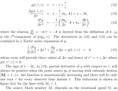
Figure 2: Influence of Mach number onτ(t),tandτ non-dimensionlaised over the period
T = 2Ωπ: a) Variation ofτ(t) withM and b) diagram of Cusp Catastrophe inτ, t, M.
Even for this simplified analysis, equation (11) is an implicit function ofτ and cannot be resolved analytically because the motion of the sourceyis complex and involves transcendental functions. On the other hand, although the equation is implicit in t, the motion of the observerx is always simpler than the source’s motion. The Forward Time Algorithms exploit this characteristic by definingτ and calculating the timetwhen the signal reaches the observer, i.e. propagating the signal forward in time at an instant t > τ.
In order to devise a more efficient root finder process for retarded time algorithms, it is necessary to analyse the behaviour of the functionτ(r, t) and its derivatives with respect to t. The solution of Equation (11) represents the intersection between the spherical waves centred in xOB whose radius is
varying as r = c(t−τ), and the curve in space described by the motion of the source pointyB for the same tandτ. The radiation distanceris covered
by the pressure signal in the time r/c = (t−τ), due to the finite speed of sound waves and is knows as Compressibility Delay (see 18).
The existence of single or multiple roots forτ(r, t) depends on the speed at which the source moves along the radiation vector. More precisely, this speed is defined asvS·ˆr or in terms of mach number as Mr=vS·ˆr/c. Calculating
appears Mr:
g(t, τ, r) = τ−t+r
c (12)
∂g(t, τ, r)
∂τ = 1−
1
c(vs·ˆr) = 1−Mr (13) ∂2g
∂τ2 = − 1
c
∂vs
∂τ ·ˆr+vs· ∂ˆr
∂τ
(14)
where the relation ∂r
∂yi = −r/r = −ˆr is derived from the definition of r. yi is the ithcomponent of y(y
s, τ). The derivatives in (13) and (14) can be
combined in a Taylor series expansion of g:
1 2!
∂2g
∂τ2 ∗∆τ
2+∂g
∂τ ∗∆τ +g(t, τ, r) = 0 (15)
whose roots will provide three values of ∆τ and hence ofτ∗ =τ+ ∆τ where
g(t, τ∗, r) = 0.
The sign of 1−Mr, in (13), partial derivative ofg with respect to τ, will
always be positive when the point source ys is moving with subsonic motion
|M|<1, i.e. the function is monotonically increasing and there will be only one root τ for every observer time instant t. This behaviour is shown in figure 2(a) for the lines with Mr <1.
The source Mach number Mr depends on the rotational speed Ω, on
the distance of the source from the rotation point, i.e. |ys|, and on the
sound speedc(and hence the fluid temperature) in the undistorted flow. By increasing the Mach number of the source, in the current case increasing Ω, it is possible to observe the behaviour of τ versus the corresponding t. In particular, the steepness of the curve increases, until Mr = 1, where a part
of the curve is perpendicular to the t axis.
Figure 2(b) is a three dimensional representation of Figure 2(a) and rep-resents a diagram of Cusp Catastrophe, (see 16; 17). These diagrams are obtained in the study of dynamical systems by varying the parameters of the system and following its behaviour. In this case g = 0 has only one solution for Mr ≤ 1, which for Mr ≥ 1 (here, we refer mainly to a range
of 1 ≤ Mr < 2) splits into two stable solutions and one unstable solution
(as per definition in (19)), central region of the “S” shape. Note that at
Mr >>1there can exist more than three solutions.
Along the trajectory described by the point source, rotating at Mr = 1,
[image:12.612.110.502.143.448.2]t
1
-M
r
0 0.2 0.4 0.6 0.8 1
-1 0 1 2 3 M=0.4 M=0.8 M=1.0 (a) + + + + + + X X X X X X X X t 1-M r
[image:13.612.138.462.139.299.2]0 0.2 0.4 0.6 0.8 1 -1 0 1 2 3 M=0.4 M=0.8 M=1.0 M=1.2 M=1.6 M=2.0 + X (b)
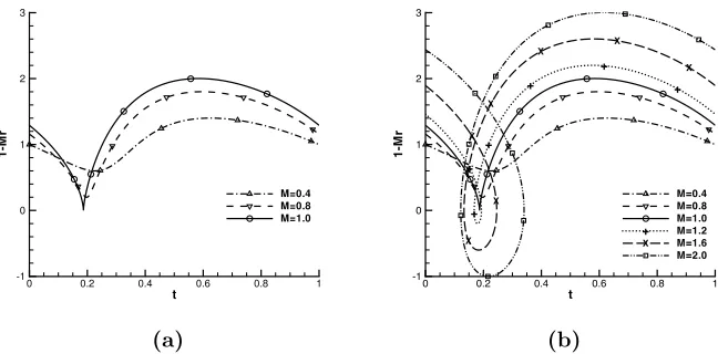
Figure 3: Behaviour of 1−Mrby varying source rotational speed Ω: a) Close up of sources withM ≤1.0 and b) sources with 0.4≤M ≤2.0.
Considering that for the chosen motion of the source ys the trajectory is
represented by a circumference of radius|ys|, the conditionMr = 1 is verified
when the radiation vector r is tangent to this path. When the source point passes from this specific position, along its trajectory, it is moving toward the observer with the same speed of its acoustic signal, i.e. the speed of sound c. The analysis of the second partial derivative of the functiongwith respect toτ will help to clarify this condition. It can be found from (14) that ∂τ∂2g2 = 0
in the same position, along the trajectory of the source, where ∂g∂τ = 0. The acceleration vector ∂vs
∂τ is always normal to the velocity vector which,
in the point ∂g∂τ = 0, is parallel to ˆr. Thus, the first dot product on the r.h.s. in (14) is 0, furthermore the second term on the r.h.s. is expanded as (M·(c/r(Mrˆr−M))) which is zero when (M||ˆr) andM = 1, i.e. in the same
point as (1−Mr = 0).
The combination of these two conditions, i.e. first and second derivatives (or Hessian determinant) equal to zero, means that the function g has a cusp in this point. A cusp is also visible in the plots of ∂g∂τ versus t for M = 1, Figure 3.
maxima, i.e. two points in which ∂τ∂t = 0 or ∂τ∂g = 0.
The meaning of the multiple positions of the emission point can be clar-ified by analysing the point source kinematics and physics. There will be three segments of the source point trajectory from which the emitted acous-tic signals will reach the observer at the same time instant. The multiple roots segments of the source point trajectory can be found in the proximity of the point where the radiation vector is tangent to ys path. It is obvious
that at the tangent pointMr will be exactlyMr =|M|. This means that the
two points in which ∂τ∂t = ∂g∂τ = 0, i.e. Mr = 1, can be found via the following
equation:
(1−Mr) = (1− |M|cosθrM) = 0
=⇒cosθrM =
1 |M|
(16)
The solution of (16) can be calculated in terms of azimuth values ψ. The two roots of this equation are at a symmetric positions with respect to the tangent point ψtn. The azimuthal distance of the two roots from ψtn tends
to increase with the increase of M and will reach a value ∆ψ as close to 90◦ as much M tends to ∞.
The functionτ(t) corresponding tog = 0 is plotted in Figure 2, for several different values of Mach number M, in the range M = 0.4 up to M = 2.0. Some more insight on the retarded time equation can be gained by looking at the plots of ∂τ∂g and ∂∂τ2g2, in Figs.3 and 4, same Mach range as the previous
figure. The first partial derivative, 1−Mr decreases reaching 0 when M = 1
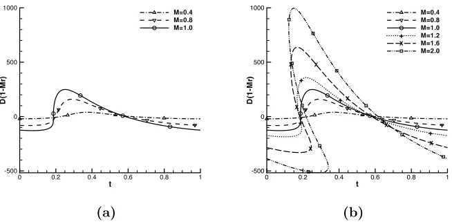
with the cusp point clearly visible. For further increase in M all the curves present a Crunode or ordinary double point defining a loop. The size of this loop increases with M and is connected to the size of the [τ, t] region having multiple τ roots for each t. Figure 4 highlights that ∂∂τ2g2 = 0 when
∂g
∂τ = 0, hence the existence of degenerate critical points for g. Furthermore,
the positive and negative values of ∂τ∂2g2 = 0 in Figure 4, suggest that the
corresponding Emission Surface F(t, τ∗) = 0 will change its curvature in the critical point.
4. Root finder algorithm
t
D
(1
-M
r)
0 0.2 0.4 0.6 0.8 1
-500 0 500 1000 M=0.4 M=0.8 M=1.0 (a) + + + + + X X X X X X X t D( 1 -Mr )
[image:15.612.137.464.139.301.2]0 0.2 0.4 0.6 0.8 1 -500 0 500 1000 M=0.4 M=0.8 M=1.0 M=1.2 M=1.6 M=2.0 + X (b)
Figure 4: Behaviour of ∂∂τ2g2 by varying source rotational speed Ω: a) Close up of sources
withM ≤1.0 and b) sources with 0.4≤M ≤2.0.
various flow conditions. The ideas which form the base for the development of the current algorithm have been introduced in the previous sections. In the following paragraphs it will be shown how the aforementioned analysis leads to the final version of the root finder algorithm implemented during this research.
The analysis of the retarded time function, τ(t), highlighted the impor-tance of ∂g∂τ, as an indicator for the behaviour of τ. For this reason the Newton algorithm was considered as the optimum starting point for the pro-posed root finder method. It is now necessary to show the issues which affect the classical algorithms making them inefficient or not suited for conditions such as supersonic source motion.
It is possible to find multiple roots by means of the classical version of Newton’s and Brent’s algorithms, but in order to do so the roots must be first bracketed. Given an interval [τ1, τ2], where supposedly the multiple roots of a generic functionf are located, the bracketing algorithm will divide the input interval in a user set Nsi number of sub intervals. The function f under
analysis will then be evaluated on the extremes of each sub interval. The process is iterated until the sub interval in which f has two opposite signs is found.
up to three multiple roots, the bracketing process must be repeated until the three sub-intervals containing the roots are found; even though for the function g, as illustrated in Figure 2, the existence of multiple roots is con-fined only in a small part of the observer time history. Hence, even when g
has single τ root, i.e. during the majority of observer time history, the root bracketing algorithm will inefficiently seek for the other two roots sweeping all the defined Nsi and thus increasing the computational time. This
pro-cess must be repeated for every observer time t along the overall observer time interval [ts, te] defined in the calculation and for all the source points
which define the integration domain of interest. This process will add many unnecessary steps to the overall computational time.
Unfortunately the root bracketing process is a fundamental step for both Newton’s and Brent’s algorithms and cannot be avoided. The only possible answer to this issue is to define a root finder method which does not require this time consuming procedure. In order to do so it is helpful to understand how the two aforementioned root finder algorithms work and why they require root bracketing. It must be remembered that for functions f(x) that are non-monotone, the two algorithms under analysis can encounter additional difficulties, (see 8), around local minima and maxima, ddfx = 0, and inflection points, dd2xf2 = 0.
The Newton method is based on a linear approximation of the function under analysis via a Taylor series expansion truncated at the first order. The method has quadratic convergence and, near the roots will converge very fast, but when the evaluation point is far from a root or close to critical points the method loses its high convergence properties and becomes linear. In the worst case the algorithm could reach a stall situation, i.e. the evaluation point starts oscillating around the function inflection point and the method cannot reach convergence. It is obvious that the closest to the root will be the first evaluation point, the faster and more certain the method will converge. Hence, the root bracketing process will play an important role in this task both for the Newton’s method convergence and for minimising the likelihood of failure in the root search. While for monotonic functions this improvement could be considered optional, in the case of non-monotonic functions the root bracketing step is indispensable. The Newton method alone will otherwise fail to provide all the required roots for such functions.
neighbourhood of a zero crossing interval. Inverse quadratic interpolation uses three prior points [xi, f(xi)] to fit an inverse quadratic function, i.e.
x as a quadratic function of f(x), whose value at f(x) = 0 is considered the next estimate of the root x. The algorithm includes also an internal root bracketing which is used in order to prevent the search from jumping outside the brackets of the input interval. Even for the Brent’s algorithm it is required a pre-step of a root bracketing algorithm in order to concentrate the search in smaller domains. Furthermore, the Brent’s method alone is not suited to compute multiple roots. Only in combination with a root bracketing algorithm, which establishes the multiple roots’ intervals, Brent’s method can find multiple roots, working separately in each sub-interval.
From the discussion above it is apparent that the main reason for which the pre-step procedure of root bracketing is required is the linear behaviour of the two methods when the evaluation point is far from the root. Furthermore, the Newton’s algorithm is better suited for monotonic functions and the Brent’s algorithm cannot provide the multiple roots without a previous search of the sub-interval in which these roots exist. A possible solution then can be to consider a method which is non-linear, i.e. which implements an higher order approximation of the function under analysis.
In helicopter rotor aeromechanic analysis, described in Sec.2, the motion of the main rotor blades can be defined via transformation matrices between the different reference frames involved. Furthermore the angles, flapping, lead/lagging and pitching are generally represented via Fourier series of the azimuth ψ =ψ(τ). For these reasons the calculations of ∂τ∂g can be obtained analytically. Thus, Newton’s method is the best candidate as a starting point for the improved root finder method developed in this research.
While in the Newton’s algorithm the Taylor series expansion of the func-tion f(x) is truncated at the first order, in the proposed approach the series is truncated at the third order. The function is thus approximated as a third order curve which is tangent to f inx. This enhances the accuracy of the approximation which will remain close to the actual function for larger intervals, with respect to the first order series.
Starting from a Taylor series expansion of g(t, τ, r) around the point τ, which is an initial estimate, and keeping constant the other variables:
g(t, τ + ∆τ, r) = g(t, τ, r) + ∂g
∂τ ∗∆τ+
+1 2!
∂2g
∂τ2 ∗∆τ 2
+1 3!
∂3g
∂τ3 ∗∆τ 3
+. . .
and imposing that the ∆τ increment will bring g →0 the following polyno-mial equation is obtained:
1 3!
∂3g
∂τ3 ∗∆τ 3+ 1
2!
∂2g
∂τ2 ∗∆τ
2 +∂g
∂τ ∗∆τ +g(t, τ, r) = 0 (18)
whose roots will provide three values of ∆τ and hence ofτ∗ =τ+ ∆τ where
g(t, τ∗, r) = 0.
In addition, by approximating the function with a 3rd order polynomial, three ∆τ are obtained instead of one. Most of the times the smallest of the three roots of the approximating Taylor series will be under the set tolerance in the first evaluation. This reduces dramatically the computational time required to solve the whole problem. The gain in computational time remains positive even when considering the additional time required by the calculation of the second and third derivatives of the function. It should be highlighted that in the present analysis, although the first order derivative was calculated analytically, the high order derivatives were calculated numerically.
The solution of the third order polynomial is another operation which could affect the efficiency and efficacy of the proposed method but, if com-puted efficiently, this process will not increase the computational cost. In the proposed algorithm, the solution of the third order polynomial is obtained by implementing a fast analytical method capable of providing the three roots with a limited number of operations. This analytical method is based on an approach recently proposed by (20), which is similar to the classical solution of the second order polynomials. A brief description of this solution follows in the paragraphs below, further details can be found in (20).
Considering a generic third order polynomial y(x)
y = ax3+bx2+cx+d (19)
but introduces the following parameters:
δ= b
2−3ac
9a2
h= 2aδ3 λ= 3δ2
xN =
−b
3a yN =ax3N +bx
2
N +cxN +d
(20)
These parameters are characteristic of the particular polynomial and are used first to define the expected root patterns, e.g. one real and 2 complex roots or three real roots etc., and then to evaluate the roots. Essentially, these parameters reveal how the solution is connected to the curve’s geometry. The Nickalls’ method can evaluate the roots of a generic third order polynomial more efficiently than the classical third order Cardano method.
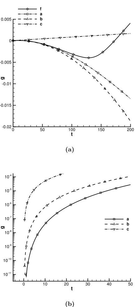
The third order polynomial approximation enables one to findτ∗ even if the evaluation pointτ is not very close to the root. This is a great advantage compared to the classical Newton’s method which requires close proximity to the root in order to accelerate the convergence. In Figure 5 it is evident that the approximation errors between the Π(τ) and g(τ) is, on average, 2 or 3 orders of magnitude smaller with respect to the linear method. In most of the cases, using Π3, the approximate root of g is already below the set tolerance in the first evaluation. For those cases when this does not happen, it is possible to converge under the limit tolerance by including just one iteration of the linear Newton’s method.
Furthermore the three ∆τ roots of the polynomial can be ordered by increasing magnitude. The first, smallest, ∆τ represents the actual increment required to reach the closest root of the function under analysis. For cases when g has multiple roots, the second ∆τ represents a fairly good estimate of the second closest multiple root of g.
5. Improved Retarded Time Algorithm
The classic retarded time algorithms are based on the following steps:
• define a starting observer timetsand a constant positive time increment
t
g
0 50 100 150 200
-0.02 -0.015 -0.01 -0.005 0 0.005
f a b c
(a)
t
g
0 10 20 30 40 50
10-11
10-10
10-9
10-8
10-7
10-6
10-5
10-4
a b c
[image:20.612.191.408.126.618.2](b)
Figure 5: Function g(τ) and approximating polynomials Π(τ) along with the relative errors. (Π3(τ) is the 3rd order polynomial, ∆τ0= Ω∗2360π ): a)g(τ) and approx polynomials
• find for ts+i∗∆t, i = 0, Nt the time τ for which g(t, τ, r) = 0, and if
M > 1 search for 3 roots;
• if t =te stop.
By using the steps described above, the search for multiple roots, when
M > 1, will be performed in any case whether or not they exist. This will waste a lot of computational time in those intervals where only one single root is available. As can be seen from Figure 2, in the cases of supersonic motion there is a t range where, increasing τ the observer time t first increases then decreases and then finally increases again. Thus, for a positive increment of
τ the corresponding increment in t is not always positive.
This observation suggests an approach for the solution of the retarded time equation. The definition of the ∆tsign should not be constant and hard-coded in the algorithm but should lean on the behaviour of the retarded time function. An improvement in the efficiency of the standard retarded time algorithm can be obtained by using an increment ∆t which is not always positive but can also be negative or zero when required.
It is possible to do this by adding one more step to the base algorithm described above. During this step, given the approximating polynomial in the pointg(t, τ∗, r), the algorithm verifies wether a new approximating poly-nomial computed in g(t+ ∆t, τ∗, r) can be solved. Then, the adjustments on ∆t sign are made based on the results from this query. The sign must change in order to sweep the τ(t) curve along the positive direction ofτ. The value ∆t= 0 instead is necessary to take into account those instants when g
derivative, i.e. 1−Mr, is 0. ∆t will change sign just after these instants.
Exploiting the aforementioned idea it is possible to reduce the multiple roots search to a single root search. The other roots will be obtained by sweeping τ along its “S” shaped curve, i.e. varying ∆t. Furthermore, it is not necessary to know the number of roots, and hence emission surface branches, a priori. The right number of roots in the [ts, te] will be obtained by
the sweeping process. All these features make the improved algorithm more efficient and better suited to handle both subsonic and supersonic motions.
the search. In the following section the comparisons with the Newton’s and Brent’s algorithms are presented.
6. Comparison of Root finder algorithms
A rotating point source, or panel, represents an optimum case for compar-ing the performance of each of the different root finder methods. Considercompar-ing a point P1 which is in a Reference Frame Rf rotating with respect to the ground fixed frame, the kinematics ofP1 can be described with the equation:
r = (xOB−([TGR])yP1) (21)
Which is obtained by assuming VH = VOB =0 in equation (10) and by
considering only the rotational motion of P1. Given the different behaviour of the retarded time roots in subsonic and supersonic regimes, the analysis will consider both regimes.
Although the above equation is much simpler with respect to the com-plete equation (7), it is still not possible to obtain an analytical solution for
g(t, τ, r) = 0. For this reason, the results from the different root finder algo-rithms must be compared with the numerical solution obtained via a Forward or “Advanced” time approach. The Forward time equation, t(τ) can easily be solved numerically, and in the case of a stationary observer it is possible to obtain an analytical solution for t(τg=0). Hence, the Advanced time nu-merical solution, could be considered equivalent to the analytical solution of
τ(t), through the solution of the inverse problem t(τ).
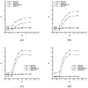
Figure 6 illustrates the computational cost for each approach considered for the solution of the solution of rotating panels (HelicA identifies the ap-proach proposed in this paper). The Mach number is evaluated at the centre of the panel and the computational time is normalised dividing by the compu-tational time of the Advanced Time solution. The variation in Mach number is obtained by increasing the rotational speed ω. The number of intervals which is specified in Figure 6 represents the number of sub-intervals used in the bracketing step. This step is a requirement of the two classic meth-ods, and while in subsonic conditions only 2 sub-intervals are used for both methods, in the supersonic regime the number of interval must be 2 orders of magnitude larger.
m
q
0 0.5 1 1.5 2 2.5 3 3.5 4 0 1 2 3 4 5 6
7 ADV 5P
HelicA 5P Newt-Raph 1P Brent 1P (a) m q
0 0.5 1 1.5 2 2.5 3 3.5 4 0 1 2 3 4 5 6
7 ADV 5P
HelicA 5P Newt-Raph 1P Brent 1P (b) m q
0 0.5 1 1.5 2 2.5 3 3.5 4 0 1 2 3 4 5 6 7 ADV 5P HelicA 5P Newt-Raph 1P Zbrent 1P (c) m q
0 0.5 1 1.5 2 2.5 3 3.5 4
[image:23.612.128.466.188.527.2]0 2 4 6 8 10 12 14 ADV 5P HelicA 5P Newt-Raph 5P Zbrent 5P (d)
algorithm for different panel geometries and observer positions. By consid-ering 500 configurations the dependence on the aforementioned parameters is effectively averaged out from the results.
Observing the plots in subsonic regime, it is clear that all the algorithms require a similar computational time. Under these conditions, the Brent’s algorithm provides the faster solution, but it should be highlighted that both Newton and Brent’s methods consider only the panel centre in the solution. This is reported in the legend of Figure 6 with 1P, i.e. 1 point per panel. On the other hand the “Advanced Time” and the HelicA algorithms were executed considering 5P points per panel, the centre and the four panel vertices.
In Figure 6(d) the Newton’s and Brent’s algorithms were implemented resolving the same number of points per panel as the other two methods. The novel root finder algorithm performs faster than the classical methods, also in the subsonic regime; the computational time for the classical methods is comparable to the Advanced Time algorithm.
A more complex challenge arises when the sources are in supersonic mo-tion, due to the existence of multiple retarded times τ and positions y(τ) corresponding to a single point sourcey0 and observer timet. This increased complexity is visible in Figure 6, where a steep gradient and a sudden increase in computational time is evident in the curves representing the two classical methods for M ≈1. This is due to the increase in the number of bracketing sub-intervals which is required in order to find all the multiple roots for a given observer time. The computational time increases proportional to the number of sub-intervals considered.
When a low number of sub-intervals is used during the bracketing step, the solutions obtained with the Newton’s and Brent’s algorithms do not capture the multiple τ roots for all the different Mach numbers. Hence, increasing the number of sub-intervals in the bracketing step has a positive effect on the search of multiple roots. In Figure 6, only the calculations performed with 400 sub-intervals could provide the multiple roots for all the supersonic conditions.
On the other hand, the Advanced Time and the root finder algorithm proposed in the present study do not show a strong dependence on the Mach number. The computational time required by the above method remains al-most constant and around 10 to 20% higher with respect to the time required by the Advanced Time algorithm.
x x x x
x x x
x x x
x x x
x x x
x x
x x x x
x
q
z
0.1 0.15 0.2 0.25
0 0.2 0.4 0.6
0.8 ADV
HelicA Newton-Raph Brent
[image:25.612.134.459.239.538.2]x
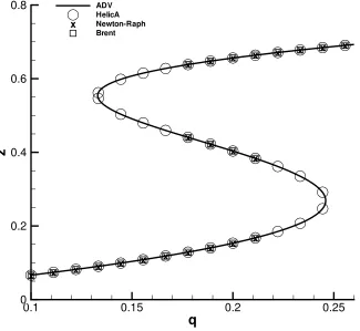
Figure 7: Solution of τ(t) via different root finder algorithms,M = 1.6 (non dimensional
classical methods, it is evident the much higher computational time required by the latter two approaches, more than 5 times. Furthermore, in Figure 7 it is clear that both Newton’s and Brent’s algorithms do not capture the full range of multiple roots τ, while the proposed algorithm follows closely the Advanced Time prediction. The two classical algorithms fail to identify the roots close to the local minimum and maximum of the inverse function
t(τ), where the roots become so close to each other that they fall in the same sub-interval of the bracketing step. A possible solution to this problem could be to deploy an even finer sub-interval bracketing step, which in this case was executed with a value of 400 sub-intervals.
7. Conclusions
A novel approach for the search of theτ roots of the retarded time func-tion has been presented in this paper. The approach is based on some consid-erations on the kinematics of rotating sources such as helicopter rotors, and on the bifurcation analysis of the retarded time functiong(t, τ, r). From these ideas it was possible to define a novel root finder algorithm, which extends the Newton’s method, using a Taylor series truncated to the third order, and exploits the Nickalls method for the solution of third order polynomials.
The additional requirements in computational time, due to the calcula-tions of the higher order terms in the Taylor series and to the solution of the third order polynomial, are overcome by the increased overall performance and efficiency of the proposed method. In fact, the algorithm was imple-mented numerically and its performance was compared to the Newton’s and Brent’s algorithms. From the comparisons it is clear that the proposed ap-proach is faster and more efficient with respect to the two classical methods, especially in the presence of sources rotating supersonically. More precisely the overall computational time required by the proposed method is compa-rable to that required by a Forward time solution and can be up to 5 times faster than the classical root finders.
[1] J. E. Ffowcs Williams, D. L. Hawkings, Sound Generation by Turbulence and Surfaces in Arbitrary Motion, Philosophical Transactions of the Royal Society of London. Series A, Mathematical and Physical Sciences 264 (1151) (1969) 321–342.
Analogy and Kirchoff Formulation for Moving Surfaces, AIAA Journal 36 (8) (1998) 1379–1386.
[3] K. S. Brentner, F. Farassat, Modeling aerodynamically generated sound of helicopter rotors, Progress in Aerospace Sciences 39 (2003) 83–120.
[4] P. di Francescantonio, A New Boundary Integral Formulation for the Prediction of Sound Radiation, Journal of Sound and Vibration 202 (4) (1997) 491–509.
[5] F. Farassat, Discontinuities in Aerodynamics and Aerocoustics: the Concept and Application of Generalized Derivatives, Journal of Sound and Vibration 55 (2) (1977) 165–193.
[6] F. Farassat, Introduction to Generalized Function with Applications in Aerodynamics and Aeroacoustics, Tech. rep., NASA Technical Paper 3428 (1996).
[7] F. Farassat, Theory of Noise Generation from Moving Bodies with an Application to Helicopter Rotors, Tech. rep., NASA TR R-451 (1975).
[8] W. H. Press, S. A. Teukolsky, W. T. Vetterling, B. P. Flannery, Numeri-cal Recipes in FORTRAN; The Art of Scientific Computing, Cambridge University Press, New York, NY, USA, 1993.
[9] A. S. Lyrintzis, Surface Integral Methods in Computational Aeroacous-tics - From the (CFD) near-field to the (Acoustic) far-field , International Journal of Aeroacoustics 2 (2) (2003) 95–128.
[10] I. Abalakin, V. Anikin, P. Bakhvalov, V. Bobkov, T. Kozubskaya, Nu-merical investigation of the aerodynamic and acoustical properties of a shrouded rotor, Fluid Dynamics 51 (3) (2016) 419–433.
[11] I. Abalakin, P. Bahvalov, V. Bobkov, T. Kozubskaya, V. Anikin, Numer-ical simulation of aerodynamic and acoustic characteristics of a ducted rotor, Mathematical Models and Computer Simulations 8 (3) (2016) 309–324.
[13] E. Ntumy, S. Utyuzhnikov, Active sound control in 3D bounded regions, Wave Motion 51 (2) (2014) 284–295.
[14] J. G. Leishman, Principles of Helicopter Aerodynamics, 1st Edition, Cambridge University Press, 2000.
[15] K. S. Brentner, Prediction of Helicoptr Rotor Discrete Frequency Noise, Tech. rep., NASA TM-87721 (1986).
[16] R. Gilmore, Catastrophe Theory for Scientists and Engineers, Dover Publications, New York, 1993.
[17] T. Poston, Catastrophe Theory and Its Applications, Dover Publica-tions, New York, 1997.
[18] S. Ianniello, New perspectives in the use of the Ffowcs Williams Hawk-ings equation for aeroacoustic analysis of rotating blades, Journal of Fluid Mechanics 570 (2007) 79–127.
[19] E. Zeeman, Catastrophe Theory, Scientific American 234 (4) (1976) 65– 83.