PRECONDITIONING AND ITERATIVE SOLUTION OF ALL-AT-ONCE SYSTEMS FOR
1
EVOLUTIONARY PARTIAL DIFFERENTIAL EQUATIONS
2
ELEANOR MCDONALD ∗
, JENNIFER PESTANA†, AND ANDY WATHEN∗
3
Abstract. Standard Krylov subspace solvers for self-adjoint problems have rigorous convergence bounds based solely 4
on eigenvalues. However, for non-self-adjoint problems, eigenvalues do not determine behavior even for widely used iterative 5
methods. In this paper, we discuss time-dependent PDE problems, which are always non-self-adjoint. We propose a block 6
circulant preconditioner for the all-at-once evolutionary PDE system which has block Toeplitz structure. Through reordering of 7
variables to obtain a symmetric system, we are able to rigorously establish convergence bounds for MINRES which guarantee 8
a number of iterations independent of the number of time-steps for the all-at-once system. If the spatial differential operators 9
are simultaneously diagonalizable, we are able to quickly apply the preconditioner through use of a sine transform, and for 10
those that are not, we are able to use an algebraic multigrid process to provide a good approximation. Results are presented 11
for solution to both the heat and convection diffusion equations. 12
Key words. evolutionary equations, Toeplitz matrix, circulant preconditioner, iterative methods, block matrices 13
AMS subject classifications. 65F08, 15B05, 65M22 14
1. Introduction. It is widely appreciated that self-adjoint problems are, in some respects, easier to
15
solve than problems without natural symmetry. Not least, theoretical understanding is greater than for
non-16
self-adjoint problems, so that, for example, there are linear algebra solution methods—conjugate gradients
17
[22] and MINRES [37]—for large scale symmetric problems for which descriptive and guaranteed convergence
18
bounds based only on eigenvalues exist. For non-symmetric discretized problems there are no generally
19
descriptive convergence bounds, and eigenvalues do not guarantee anything: Greenbaum, Pt`ak and Strakoˇs
20
[18] have proved even for the widely used GMRES method that essentially any convergence curve is possible
21
for a problem regardless of its eigenvalues.
22
This stark difference means, for example, that one has rigorous theory to guide the design of
precondi-23
tioners for symmetric problems, but preconditioners for non-symmetric problems must essentially be designed
24
based on heuristics (see [47]). Thus the important multigrid and domain decomposition paradigms are
rig-25
orously underpinned and guarantee rapid solvers for symmetric problems, by contrast to non-self-adjoint
26
problems. Further, parallelization must yield the expected benefits for symmetric problems.
27
One important class of non-self-adjoint problems arise from first order time evolution: an initial value problem for a time-dependent PDE has an adjoint that is a final value problem since
⟨ut, v⟩ = −⟨u, vt⟩.
This is true regardless of whether the spatial operator is self-adjoint. Via time-stepping (the method of lines),
28
such problems are generally solved one time-step at a time, i.e. in a fully sequential manner. Effective (often
29
parallel) solvers for the spatial partial differential operators at each time step are widely studied and offer
30
practical solution approaches. From this perspective, it can be possible to design solvers that have excellent
31
scalability with respect to the number of spatial degrees of freedom,n, but computational effort must depend
32
on the number of time-steps,`. There has also been significant work on methods that parallelize over time,
33
e.g. [7, 11, 19, 29, 42]. For a review of parallel-in-time methods, see [14]. Our method falls into the class
34
of space-time, or all-at-once, algorithms that solve for all time-steps simultaneously. Such methods include
35
the parareal method [17, 26], space-time multigrid [16, 20, 23] and multigrid-reduction-in-time [12]. Our
36
approach is most closely aligned with methods in which the space-time problem is written as a monolithic
37
linear system, e.g. [1,16,20,23,28], but our method differs in the way in which this system is solved. Here,
38
we exploit the block Toeplitz structure of the resulting linear system to develop new preconditioners for
39
which the number of Krylov iterations is independent of the number of time-steps`. We note that work by
40
Gander et al [15] presents a complementary all-at-once approach that requires all time-steps to be distinct
41
to ensure diagonalizability. Instead, we consider the case that all time-steps are the same.
42
∗Oxford University Mathematical Institute ([email protected],[email protected]).
†Department of Mathematics and Statistics, University of Strathclyde ([email protected]). This author was supported by Engineering and Physical Sciences Research Council grant EP/I005293.
The approach is based on the block Toeplitz structure of evolutionary problems that allows
symmetriza-43
tion, so that the MINRES method of Paige and Saunders [37], which is designed for symmetric problems,
44
can be correctly applied—convergence then only depends on eigenvalues. After applying block circulant
pre-45
conditioners to the symmetrized system we prove clustering of eigenvalues so that rapid (and`-independent)
46
convergence is rigorously guaranteed. The relevant computations with circulants are either trivial or
al-47
most optimally effected by a fast Fourier transform (FFT). We provide a brief overview to circulant based
48
preconditioning in Section2.
49
Our approach is best introduced in terms of a simple application, hence this is described in Section3.
50
The aspects of symmetrization are covered in Section4. For non-self adjoint spatial operators, we are still
51
able to obtain eigenvalue estimates based on the LSQR algorithm (also due to Paige and Saunders [38]),
52
which are described in Section 5. Numerical results are presented for the heat and convection-diffusion
53
equations in Section6with our conclusions in Section7.
54
2. Circulant preconditioning. In order to motivate our block circulant based preconditioner, we first
55
introduce circulant preconditioners for general Toeplitz matrices. LetT∈Rn×n be the nonsingular Toeplitz 56
matrix andC∈Rn×n be the nonsingular circulant preconditioner given by 57
T=
⎡⎢ ⎢⎢ ⎢⎢ ⎢⎢ ⎢⎢ ⎣
t0 t−1 ⋯ t−n+2 t−n+1
t1 t0 t−1 t−n+2
⋮ t1 t0 ⋱ ⋮
tn−2 ⋱ ⋱ t−1
tn−1 tn−2 ⋯ t1 t0
⎤⎥ ⎥⎥ ⎥⎥ ⎥⎥ ⎥⎥ ⎦
, and C=
⎡⎢ ⎢⎢ ⎢⎢ ⎢⎢ ⎢⎢ ⎣
c0 cn−1 ⋯ c2 c1
c1 c0 cn−1 c2
⋮ c1 c0 ⋱ ⋮
cn−2 ⋱ ⋱ cn−1
cn−1 cn−2 ⋯ c1 c0
⎤⎥ ⎥⎥ ⎥⎥ ⎥⎥ ⎥⎥ ⎦
.
58
For Toeplitz systems, circulant matrices have been popular preconditioners, not least because they can
59
be applied quickly using a fast Fourier transform (FFT). The matrixC has the diagonalization,C=UΛU∗
60
where, if we denote the Fourier matrix by F = (fjk), fjk =e2(j−1)(k−1)πi/n, then we have thatU =F/√n. 61
Also Λ=diag(F cn), wherecnis the first column ofC. This relationship to the FFT means that the solution 62
of a linear system with a circulant matrix can be performed inO(nlogn)operations [45].
63
The idea of preconditioning Toeplitz matrices with a circulant was first introduced independently by
64
Strang in [44] and Olkin in [35]. The so-called Strang circulant proposed was constructed by taking the
65
central band of T of width n/2 and wrapping the entries around to form a circulant. In this paper, we
66
use the Strang preconditioner, which we find to be very effective for the evolutionary problems we consider.
67
However, many other circulant preconditioners could be applied (see, e.g., the books [5,32]). One example is
68
the optimal circulant [6], which minimizes the Frobenius norm distance to the given Toeplitz matrix over all
69
possible circulants. A unifying approach to selecting the best possible circulant preconditioner was proposed
70
in [36].
71
Theoretical convergence bounds for these types of preconditioners have generally been restricted to
72
symmetric (Hermitian) positive definite Toeplitz matrices. For many existing preconditioners—including the
73
Strang and optimal preconditioners—and for wide classes of Toeplitz matrices, the preconditioned system is
74
given byC−1T =I+R+E, whereRhas small rank andEsmall norm. For non-symmetric systems this is not 75
sufficient to provide descriptive convergence estimates for standard non-symmetric solvers such as GMRES
76
or BiCGSTAB. However [40] provides rigorous convergence bounds for non-symmetric Toeplitz matrices.
77
This is done by reordering the rows or columns ofT by pre- or post-multiplying by the Hankel matrix,
78
Y =
⎡⎢ ⎢⎢ ⎢⎢ ⎢⎢ ⎣
1 1
⋰
1
⎤⎥ ⎥⎥ ⎥⎥ ⎥⎥ ⎦
.
79
This results in a symmetric system for any Toeplitz matrix. We extend this method to our block matrix
80
setting in Section 4. We note that other preconditioning methods have been developed for non-symmetric
81
block Toeplitz structures such as those discussed in [24]. That work, however, focusses on small sized blocks
82
and is not motivated by time-dependent problems as is the case here. Furthermore, this method does not
83
include symmetrization techniques that we employ. We note that it is possible to use LSQR or LSMR [13] to
84
obtain rigorous convergence bounds for non-symmetric Toeplitz matrices, but for scalar Toeplitz problems
85
these methods are typically slower than using symmetrization and MINRES.
86
3. Motivation and model problem. In order to describe our method, we will begin by considering
87
the solution of the linear diffusion (or heat) equation initial-boundary value problem,
88
(1)
ut=∆u+f in Ω× (0, T], Ω⊂R2 orR3,
u=g on∂Ω,
u(x,0) =u0(x) att=0. 89
To solve this system, we discretize in both space and time. For simplicity, we will describe our approach
90
using a finite element discretization in space and a Backward Euler discretization in time. In practice other
91
implicit time stepping schemes and spatial discretization schemes can be used, and this will be discussed in
92
more detail later.
93
We discretize the spatial domain with a representative mesh sizehand take` time steps of sizeτ such
94
that`τ =T. This discretization of (1) gives that
95
Muk−uk−1
τ +Kuk=fk, k=1, . . . , `,
96
where M ∈Rn×n is the standard finite element mass matrix, K∈Rn×n is the stiffness matrix (the discrete 97
Laplacian) and n is the number of spatial degrees of freedom. We assume that M and K are symmetric
98
positive definite matrices. The initial vector u0 should be obtained from the initial data by a convenient
99
projection. Rearranging, we have that
100
(2) (M+τ K)uk=Muk−1+τfk, k=1, . . . , `.
101
We can solve for all time steps of such a system simultaneously using an ‘all-at-once’ approach.
Con-102
ceptually, we construct the following linear system, which defines the solution at all time steps:
103
ABEx∶= ⎡⎢ ⎢⎢ ⎢⎢ ⎢⎢ ⎣
A0
A1 A0
⋱ ⋱
A1 A0 ⎤⎥ ⎥⎥ ⎥⎥ ⎥⎥ ⎦ ⎡⎢ ⎢⎢ ⎢⎢ ⎢⎢ ⎣
u1
u2 ⋮
u` ⎤⎥ ⎥⎥ ⎥⎥ ⎥⎥ ⎦
= ⎡⎢ ⎢⎢ ⎢⎢ ⎢⎢ ⎣
Mu0+τf1
τf2 ⋮
τf` ⎤⎥ ⎥⎥ ⎥⎥ ⎥⎥ ⎦
∶=b, (3)
104
105
where A0 =M +τ K is symmetric positive definite andA1= −M is symmetric negative definite. We note 106
thatABE is now an immensen`×n`matrix; the construction ofABE only requires copies ofA0andA1and 107
is never done explicitly.
108
The matrix ABE is clearly block Toeplitz and we wish to precondition it with the associated block 109
Strang circulant matrix. AsABE is already lower triangular with just one subdiagonal, the Strang circulant 110
simply consists of wrapping the subdiagonal entry A1 around to create a circulant. Thus our proposed 111
preconditioner is given by
112
PBE∶= ⎡⎢ ⎢⎢ ⎢⎢ ⎢⎢ ⎣
A0 A1
A1 A0
⋱ ⋱
A1 A0 ⎤⎥ ⎥⎥ ⎥⎥ ⎥⎥ ⎦
.
113
In order to describe the preconditioned system, we make the observation that PBE is a rankn pertur-114
bation ofABE, sincePBE= ABE+E1A1E`T, whereEi=ei⊗In withei denoting the i-th column ofI` and 115
⊗denoting the Kronecker product. We can now examine the eigenvalues of the preconditioned system.
116
Theorem 1. The preconditioned system is equal to PBEA−1 BE =In`− ABE−1 E1Z−1E`T, which is a rank 117
n perturbation of the identity matrix In` ∈Rn`×n`, where Z =A−11+ (A
−1
BE)`−1 and(ABE)−1 `−1=E`TA
−1 BEE1. 118
Furthermore, P−1
BEABE has (`−1)n eigenvalues equal to 1 and n eigenvalues equal to the eigenvalues of 119
In− (A−BE1 )`−1Z −1.
120
Proof. WritingPBE= ABE+E1A1E`T, then by the Sherman-Morrison-Woodbury formula we have that 121
P−1
BE= (ABE+E1A1E`T)
−1= A−1
BE− A
−1
BEE1(A−11+E T `A
−1
BEE1)−1ET`A
−1
BE, 122
and thus,
123
PBEA−1
BE =In`− A−BE1 E1(A−11+E T `A
−1
BEE1)−1E`T. 124
Since A−1
BEE1(A−11+E`TA
−1
BEE1)−1E`T is of rank n, this shows that the preconditioned system is a rank n 125
perturbation of the identity. Noting that the inverse of ABE will also be block lower triangular and block 126
Toeplitz, and lettingZ=A−1 1 +E`TA
−1
BEE1, then we have that 127
P−1
BEABE=In`− ABE−1 E1Z−1E`T 128
=In`− ⎡⎢ ⎢⎢ ⎢⎢ ⎢⎢ ⎣
(A−BE)1
0 (A−BE)1
1 (A−BE1 )0
⋱ ⋱
(A−BE)1
`−1 (A
−1
BE)1 (A−BE1 )0 ⎤⎥ ⎥⎥ ⎥⎥ ⎥⎥ ⎦ ⎡⎢ ⎢⎢ ⎢⎢ ⎢⎢ ⎣
Z−1⎤⎥
⎥⎥ ⎥⎥ ⎥⎥ ⎦ 129
= ⎡⎢ ⎢⎢ ⎢⎢ ⎢⎢ ⎣
In −(A−BE1 )0Z−1
In −(A−BE1 )1Z−1
⋱ ⋮
In− (A−BE1 )`−1Z−1 ⎤⎥ ⎥⎥ ⎥⎥ ⎥⎥ ⎦
,
130
131
from which we can easily see that the eigenvalues of PBEA−1
BE are (`−1)n copies of 1 as well as the n 132
eigenvalues ofIn− (A−BE1 )`−1Z−1. 133
In fact, we can further describe the eigenvalues ofIn−(A−BE1 )`−1Z
−1in terms of the matricesA
0andA1. 134
Theorem 2. If µ is an eigenvalue of A−1
1 A0 then µ ≠ ±1 and µ `
µ`+(−1)`−1 is an eigenvalue of In − 135
(A−BE)1 `−1Z−1. 136
Proof. Firstly, a simple inductive argument can be used to show that(A−1
BE)k−1= (−1)
k−1(A−1
0 A1)k−1A−01 137
for allk=1, . . . , `. Thus we have that
138
In− (A−BE1 )`−1Z−1=In− (A−BE1 )`−1(A−11+ (A
−1
BE)`−1)−1 139
=In− [A−11(A
−1
BE)
−1
`−1+In] −1 140
=In− [(−1)`−1(A1−1A0)`+In]
−1 .
141 142
Now, A−1
1 A0 = −(In+τ M−1K) with M and K both symmetric positive definite. Thus, if µ is an 143
eigenvalue ofA−1
1 A0 thenµ≠ ±1, and there exists a nonzero vectorx∈Rn such that 144
A−1
1 A0x =µx 145
[In+ (−1)`−1(A−11A0)`]
−1
x= 1
1+ (−1)`−1µ`x 146
[In− [In+ (−1)`−1(A−11A0)`]−1]x=
µ` µ`+ (−1)`−1x,
147
which completes the proof.
148
This shows that althoughP−1
BEABEhasneigenvalues not equal to one, ifµis large then these eigenvalues 149
can cluster very close to one. In the case of the heat equation, we see that the largest eigenvalues ofA−1
1 A0 150
grow with h−2, whereh is the grid size, and therefore we see extremely clustered eigenvalues in practice.
151
Figure1 shows the eigenvalues ofP−1
BEABE for a small system. 152
We will now show thatP−1
BEABE is diagonalizable. 153
Theorem 3. The matrix PBE−1 ABE is diagonalizable. 154
Fig. 1: The eigenvalues ofPBEA−1
BE withn=81,`=10 andτ=0.1. There are 32 eigenvalues approximately
equal to 1.6275.
i
100 200 300 400 500 600 700 800 6i
0.9 1 1.1 1.2 1.3 1.4 1.5 1.6 1.7
Proof. Recall thatA−1
1 A0= −(In+τ M−1K), withM,Ksymmetric positive definite. From the proof of 155
Theorem2 we have that
156
(A−1
BE)`−1Z −1= [
In− (In+τ M−1K)`]−1, 157
which is diagonalizable and has real, negative eigenvalues. Thus, In− (A−BE)1 `−1Z
−1 is diagonalizable, and
158
has eigenvalues that are real and larger than 1.
159
LetIn− (A−BE1 )`−1Z
−1 have diagonalizationV DV−1. ThenP−1
BEABE has the diagonalizationVDV−1, 160
V = ⎡⎢ ⎢⎢ ⎢⎢ ⎢⎢ ⎢⎢ ⎣
I V0
I V1
⋱ ⋮
I V`−2
V
⎤⎥ ⎥⎥ ⎥⎥ ⎥⎥ ⎥⎥ ⎦
, and D =
⎡⎢ ⎢⎢ ⎢⎢ ⎢⎢ ⎢⎢ ⎣
I I
I
⋱
D
⎤⎥ ⎥⎥ ⎥⎥ ⎥⎥ ⎥⎥ ⎦ 161
whereVi= (A−BE1 )iZ−1V(D−In)−1. 162
Theorem1shows that GMRES will terminate withinn+1 iterations, while diagonalizability ofPBEA−1 BE 163
may help us to estimate the rate of convergence. Analogous results to Theorem1 exist for more complex
164
time-stepping schemes, as we discuss in Section 3.2. However, in these cases it is not obvious whether
165
the preconditioned matrix is diagonalizable, nor when we can expect convergence in fewer steps because of
166
eigenvalue clustering. Furthermore, Theorem 3 will not necessarily be applicable if the preconditioner is
167
applied approximately, such as with a multigrid method.
168
Although we have now demonstrated that the preconditioned system has a number of non-unit
eigenval-169
ues independent of the number of time-steps`, the circulant preconditioner we have proposed is, in principle,
170
just as difficult to invert as the original matrixA. In order to demonstrate an easy, and indeed parallelizable,
171
method of invertingP we will now consider the matrices in Kronecker product notation.
172
3.1. Kronecker product form. The block structure of the matrices allows us to describe them in
173
Kronecker product form as
174
ABE=I`⊗A0+Σ⊗A1, 175
PBE=I`⊗A0+C1⊗A1, 176
177
where
178
Σ=
⎡⎢ ⎢⎢ ⎢⎢ ⎢⎢ ⎣
0 1 0
⋱ ⋱
1 0
⎤⎥ ⎥⎥ ⎥⎥ ⎥⎥ ⎦
, C1= ⎡⎢ ⎢⎢ ⎢⎢ ⎢⎢ ⎣
0 1
1 0
⋱ ⋱
1 0
⎤⎥ ⎥⎥ ⎥⎥ ⎥⎥ ⎦
,
179
andI` is the identity matrix of dimension `×`. As described in Section 2 we can apply C1=UΛU∗ or its 180
inverse to a vector using the FFT. We define the diagonal entries of Λ to beλk,k=1, . . . , `, and note that 181
in general they are complex. Furthermore, for this very specific circulant, the eigenvalues are in fact the `
182
roots of unity, so thatλk=e2πik/`. 183
The Kronecker product has the property that(W⊗X)(Y⊗Z) = (W Y ⊗XZ). Using this, and the fact
184
thatU is unitary, allows us to rewrite the preconditionerPBE as 185
PBE=I`⊗A0+C1⊗A1= (U⊗In)[I`⊗A0+Λ⊗A1](U∗⊗In) 186
and therefore,
187
P−1
BE= (U⊗In)[I`⊗A0+Λ⊗A1]−1(U∗⊗In). 188
A similar formulation was used in [21] to write a semi-circulant preconditioner.
189
Applying the inverse of PBE to a vector requires us to multiply by U⊗In or U∗⊗In and invert the 190
block diagonal matrixI`⊗A0+Λ⊗A1. To applyU⊗In we can first apply a column and row permutation 191
that allows us to instead multiply by the block diagonal matrix In⊗U, which has n blocks of size `×`. 192
Finally, we must reverse the row and column permutation. Since the required permutation, which is a simple
193
reordering of the spatial and temporal degrees of freedom, is known in advance, multiplication by U⊗In 194
or U∗⊗I
n could be parallelizable overn processors although communication between processors would be 195
required because of the permutations.
196
The matrixI`⊗A0+Λ⊗A1is block diagonal and therefore could be inverted in parallel over`processors. 197
This matrix is complex symmetric and therefore a method such as a complex algebraic multigrid, e.g. [25,
198
27,33,41], could be used to approximately perform this step.
199
3.1.1. Simultaneous diagonalization. For our formulation of the heat equation, the blocksA0 and 200
A1 in (3) are symmetric. As we show below, the mass and stiffness matricesM and Kalso commute. As a 201
result,A0 and A1 commute, and so can be simultaneously diagonalized. The property allows us to further 202
simplify the manner in which we applyPBE. 203
If we letA0=XΦXT andA1=XΨXT then we have 204
(4) P−1
BE= (U⊗In)(I`⊗X)[I`⊗Φ+Λ⊗Ψ]−1(I`⊗XT)(U∗⊗In). 205
Now to apply the inverse of I`⊗A0+Λ⊗A1, we first need to apply (I`⊗X), which is a block diagonal 206
matrix and could be applied over`separate processors. We then invertI`⊗Φ+Λ⊗Ψ, which is diagonal and 207
therefore trivial, before applying(I`⊗XT), which is again block diagonal. Thus when we have this property, 208
the application of a circulant preconditioner becomes much cheaper.
209
If we use a finite element formulation to discretize (1) thenM andK are simultaneously diagonalizable
210
if we use a uniform square grid. For finite difference methods, the finite element mass matrix is replaced by
211
the identity matrix and therefore will always commute with the diffusion operatorK. We note that for the
212
Dirichlet problem discretized by finite elements with uniform grids we are able to compute the diagonalization
213
using sine transforms as we now describe.
214
For thexand y directions respectively, thei-th element of thej-th normalized eigenvector is given by
215
Vx(i, j) =
√ 2
nx+1sin( ijπ
nx+1), Vy(i, j) =
√ 2
ny+1sin( ijπ
ny+1), where nx is the number of interior nodes in the 216
x-direction andny is the number of interior nodes in they-direction. We construct Xx∈R(nx+2)×(nx+2) and
217
Xy∈R(ny+2)×(ny+2) by embedding each matrix within an identity matrix such that:
218
Xx= ⎡⎢ ⎢⎢ ⎢⎢ ⎣
1 Vx
1
⎤⎥ ⎥⎥ ⎥⎥ ⎦
, Xy= ⎡⎢ ⎢⎢ ⎢⎢ ⎣
1 Vy
1
⎤⎥ ⎥⎥ ⎥⎥ ⎦
.
219
We then form the two-dimensional eigenvectorsX by the simple relationX =Xx⊗Xy. As a result, we can 220
applyX to a vector using discrete sine transforms.
221
We will now examine the effect that more complex time-stepping schemes have on the system.
222
3.2. Multi step methods. For simplicity, we discretized (1) using a Backward Euler time stepping
223
scheme. However other implicit time stepping schemes could also be used. In this section we describe how the
224
ideas in the previous sections can be extended to ap-step scheme, which means thatAhaspsubdiagonals.
225
Define Ato be the following`n×`nblock lower triangular Toeplitz matrix formed of` blocks ofn×n
226
matrices withp≤`−1 subdiagonals, and define P to be corresponding Strang circulant:
227
(5) A ∶=
⎡⎢ ⎢⎢ ⎢⎢ ⎢⎢ ⎢⎢ ⎢⎢ ⎣ A0
A1 A0
⋮ ⋱ ⋱
Ap ⋱ ⋱
⋱ A1 A0
Ap ⋯ A1 A0 ⎤⎥ ⎥⎥ ⎥⎥ ⎥⎥ ⎥⎥ ⎥⎥ ⎦
, P ∶=
⎡⎢ ⎢⎢ ⎢⎢ ⎢⎢ ⎢⎢ ⎢⎢ ⎣
A0 Ap ⋯ A2 A1
A1 A0 A2
⋮ ⋱ ⋱ ⋱ ⋮
Ap ⋱ ⋱ Ap
⋱ A1 A0
Ap ⋯ A1 A0 ⎤⎥ ⎥⎥ ⎥⎥ ⎥⎥ ⎥⎥ ⎥⎥ ⎦ . 228
Define Σi∈R`×` to be the Toeplitz matrix of zeros except for 1s on thei-th subdiagonal andCi to be 229
the corresponding Strang circulant with 1s on thei-th subdiagonal and the(`−i)-th superdiagonal.
230
By simple computation we can observe thatCi= (C1)i, and therefore if we diagonalizeC1=UΛU∗ then 231
Ci= (C1)i= (UΛU∗)i=UΛiU∗. 232
We can writeAandP in Kronecker form, which gives
233
A =I`⊗A0+ p ∑ i=1
Σi⊗Ai, 234
P =I`⊗A0+ p ∑ i=1
Ci⊗Ai= p ∑ i=0
UΛiU∗
⊗Ai. 235
236
We make the additional assumption that allAicommute with each other and are therefore simultaneously 237
diagonalizable. This will occur for any time stepping method if the spatial operators K and M commute.
238
We thus assume that we have the diagonalizationsAi=X∆iXT,X orthogonal. We can now write that 239
(6) P =
p ∑ i=0
UΛiU∗⊗A
i= (U⊗In) ⎡⎢ ⎢⎢ ⎢⎢ ⎢⎢ ⎣ G1 G2 ⋱ G` ⎤⎥ ⎥⎥ ⎥⎥ ⎥⎥ ⎦
(U∗⊗I
n) = (U⊗In)G(U∗⊗In), 240
whereG =diag(G1, . . . , G`)andGj= ∑ p i=0λ
i
jAi=X(∑ p i=0λ
i
j∆i)XT ∶=XgjXT. Furthermore, 241
G = (I`⊗X)diag(g1, . . . ,g`)(I`⊗XT), 242
where (I`⊗X)and (I`⊗XT) are block diagonal and diag(g1, . . . ,g`)is diagonal. The point here is that 243
even for multi-step methods, with simultaneous diagonalization of the spatial operators we can apply the
244
inverse of the preconditionerP using only multiplication with block diagonal matrices and the inversion of
245
a diagonal matrix, which are all extremely cheap to apply.
246
We also note that, using a similar approach to that in the proof of Theorem 1, we can write the
247
preconditioned systemP−1Aas a rank-npperturbation of the identity. Thus, GMRES converges in at most
248
np+1 steps for this problem.
249
4. Symmetrized system. Although we have been able to describe the eigenvalues of the
precondi-250
tioned system and have shown that the number of non-unit eigenvalues is independent of the number of
251
time-steps, this is not generally sufficient to ascertain the convergence rate of non-symmetric solvers such
252
as GMRES. However, if our spatial operators are symmetric and using the ideas developed in [40], we are
253
able to propose a method to rewrite our system as a symmetric one, so that we are able to use eigenvalue
254
analysis to determine convergence estimates.
255
As stated earlier, the matrix A in (5) is block Toeplitz with symmetric blocks. We note that we can
256
symmetrize any matrix of this type by pre- or post-multiplication with the following block Hankel matrix,
257
(7) Y ∶=
⎡⎢ ⎢⎢ ⎢⎢ ⎢⎢ ⎣ In ⋰ In In ⎤⎥ ⎥⎥ ⎥⎥ ⎥⎥ ⎦
Pre- or post-multiplication byY will symmetrize any block Toeplitz matrix with symmetric blocks, however
259
in generalYAdoes not equalAY. If we wish to solve the system of equationsAx=f then we can solve the
260
equations
261
(8) (YA)x= Yf orAYy=f, y= Yx.
262
However, unlike for the original system we are able to use iterative methods for symmetric systems for which
263
much better convergence estimates exist. We also note thatY andY are involutory and thus Y−1= Y.
264
In order to use a symmetric matrix solver such as MINRES we require a symmetric positive definite
265
preconditioner. One such matrix is the absolute value preconditioner [40,46]∣P∣defined as,
266
∣P∣ = (PTP)1/2 (9)
267
= [(U⊗In)G∗G(U∗⊗In)] 1/2
268
= (U⊗In)∣G∣(U∗⊗In) 269
= (U⊗X)⎡⎢⎢⎢
⎢⎢ ⎣
∣g1∣ ⋱
∣g`∣ ⎤⎥ ⎥⎥ ⎥⎥ ⎦
(U∗⊗ XT), (10)
270
wheregjis the diagonaln×nmatrix in (6) and∣gj∣is its elementwise absolute value. We note∣P∣is symmetric 271
positive definite and therefore can be used in MINRES with the symmetric form of the equation (8).
272
4.1. Eigenvalue analysis. We have now described a symmetric positive definite preconditioner for
273
the symmetrized system (8) to be implemented with MINRES. Since eigenvalues provide robust convergence
274
bounds for MINRES, unlike for GMRES, we now wish to determine the eigenvalues of the preconditioned
275
system∣P∣−1YA. That, more generally, matrices of the form ofP and∣P∣are block circulant will also prove 276
useful later in this section, hence we establish this now.
277
Lemma 1. Let R ∈Rn`×n` be any matrix of the form 278
R = (U⊗X)
⎡⎢ ⎢⎢ ⎢⎢ ⎢⎢ ⎣
d1
d2 ⋱
d` ⎤⎥ ⎥⎥ ⎥⎥ ⎥⎥ ⎦
(U∗⊗XT),
279
where U and X are as in (4), and di∈Cn×n, i=1, . . . , ` are diagonal matrices. Then R is block circulant 280
andRY = YRT, whereY is as in (7). 281
Proof. IfRrs denotes the(r, s)block of Rof sizen×n, then 282
(11) Rrs=
` ∑ k=1
urkuskXdkXT. 283
To prove that R is block circulant we need to look at the definition of each urs. Now U has as its 284
columns the eigenvectors of a circulant matrix. Thus,urs=frs/ √
`where frs=e2(r−1)(s−1)πi/`. 285
We will first show that R is block Toeplitz, that is, Rrs= R(r+1)(s+1) for all r, s∈ [1, . . . , `−1]. The
286
scalarsurkusk in (11) satisfy 287
urkusk=
1 `e
2(r−s)(k−1)πi/`=u
(r+1)ku(s+1)k.
288
SinceR(r+1)(s+1)= ∑
`
k=1u(r+1)ku(s+1)kXdkX
T, it follows thatR
rs= R(r+1)(s+1). This proves that all
diago-289
nals have constant blocks.
290
IfRis additionally block circulant, then we also require thatRr`= R(r+1)1 for allr∈ [1, . . . , `−1]. To 291
show this, note thatRr`= ∑`k=1urku`kXdkXT,with 292
urku`k=
1 `e
2(r−`)(k−1)πi/`= 1 `e
2r(k−1)πi/`= 1 `e
2r(k−1)πi/`e−2πi(1−1)(k−1)/`=u
(r+1)ku1k.
293 294
SinceR(r+1)1= ∑
`
k=1u(r+1)ku1kXdkX
T,it follows that R
r`= R(r+1)1 for allr∈ [1, . . . , `−1], from which we
295
see thatRis block circulant.
296
Finally, we prove the symmetrization propertyRY = YRT. The(r, s)block ofRY is 297
(RY)rs= Rr(`−s+1)=
` ∑ k=1
urku(`−s+1)kXdkXT, 298
while
299
(YRT)
rs= (RT)(`−r+1)s= (Rs(`−r+1))
T = ` ∑ k=1
usku(`−r+1)kXdkXT. 300
Since, for allr, s, k∈ [1, . . . , `],
301
urku(`−s−1)k= 1 `e
2(r+s−`−1)(k−1)πi/`=u
sku(`−r+1)k,
302
we see that(RY)rs= (YRT)rs= (YRT)rs, sinceY andRare real. 303
In our eigenvalue analysis, it will prove useful to relateP in (5) and∣P∣in (10). To do this we introduce
304
the real orthogonal matrix
305
̃
P = (U⊗X)
⎡⎢ ⎢⎢ ⎢⎢ ⎢⎢ ⎣
sgn(g1)
sgn(g2) ⋱
sgn(g`) ⎤⎥ ⎥⎥ ⎥⎥ ⎥⎥ ⎦
(U∗⊗XT),
306
where sgn(gj) =gj∣gj∣−1. Then, 307
(12) ∣P∣ ̃P = ̃P∣P∣ = P.
308
Since they share the same eigenvector matrixU⊗X the matrices P, ∣P∣and P̃all commute and are block
309
circulant (see Lemma1).
310
Additionally, under conditions that are met for all our numerical experiments,P̃has a real, orthogonal
311
square root, as we now show.
312
Lemma 2. Assume thatA0, . . . , Aphave real eigenvalues and that∑pi=0Aihas positive eigenvalues. When
313
` is even, additionally assume that ∑pi=0(−1)iAi has positive eigenvalues. Then P̃ has a real, orthogonal 314
matrix square root. 315
Proof. The proof proceeds in two parts. We first show that ifP̃has unit determinant thenP̃has a real,
316
orthogonal matrix square root. Then, we prove that det( ̃P) =1.
317
We begin the proof of the first part by showing that any matrix inSO(n)(the group of real orthogonal
318
matrices with unit determinant) has a real orthogonal square root. To do this we use the fact that the
319
exponential of a skew-symmetric matrix belongs to SO(n) (the group of orthogonal matrices with unit
320
determinant) and every matrix in SO(n)has a skew-symmetric matrix logarithm [4]. Thus, if B ∈SO(n)
321
thenB=eF for some skew-symmetricF, and eF/2is a real orthogonal square root of B. 322
We wish to apply this result to P̃. First, note that (12) shows that P̃ is real. Additionally, using
323
the definition of the sign function, it is clear thatP̃is orthogonal. Thus, all that remains is to show that
324
det( ̃P) =1.
325
We treat the more difficult case that` is even first. The matrix C1 has as its eigenvalues the roots of 326
unityλk=e2πki/`,k=1, . . . , `. If `is even, λ`/2= −1,λ`=1 andλk=λ`−k, k=1, . . . , `/2−1. It follows that
327
forj=1, . . . , `/2−1,
328
(g`−j)∗= p ∑ i=0
(λ`−j)i∆i= p ∑ i=0
λij∆i=gj. 329
Thus,
330
(13) det( ̃P) =
` ∏ k=1
det(sgn(gk)) =det(sgn(g`/2))det(sgn(g`))
`/2−1 ∏ k=1
det(sgn(gk)sgn(g∗k)). 331
Using the assumptions of the lemma, and the definition of the sign function, we find that det(sgn(g`/2)) =
332
1, det(sgn(g`)) =1 and sgn(gk)sgn(g∗k) =sgn(gk)(sgn(gk))∗ = In. Thus, when ` is even, (13) shows that 333
det( ̃P) =1, so that P̃has a real, orthogonal matrix square root.
334
If`is odd thenλ`=1 andλk=λ`−k,k=1, . . . ,(`−1)/2. The proof that det( ̃P) =1 then follows similarly,
335
except thatC1does not have an eigenvalue at−1. Thus, when`is odd,P̃also has a real, orthogonal matrix 336
square root.
337
We remark that the conditions of Lemma 2 are generally easy to check. When K and M in (2) are
338
positive definite, then all that is required is to compute sums involving the scalar coefficients that define the
339
time-stepping scheme. The conditions are met for all numerical experiments involving the heat equation in
340
Section6.
341
We want to look at the eigenvalues of the preconditioned system ∣P∣−1YA and we can easily see that
342
these will be the same as the eigenvalues of the matrix ∣P∣−1/2YA∣P∣−1/2 by a similarity transform. The
343
matrixY of (7) comprises`blocks, and we writeYp for the corresponding matrix withpblocks. 344
Theorem 4. Let V = [E`−p+1, . . . , E`] ∈R
n`×np and
345
(14) W =
⎡⎢ ⎢⎢ ⎢⎢ ⎢⎢ ⎣
Ap . . . A2 A1
Ap A2
⋱ ⋮
Ap ⎤⎥ ⎥⎥ ⎥⎥ ⎥⎥ ⎦
,
346
W ∈Rnp×np.Then for ∣P∣andA as defined as in (10)and (5)respectively,
∣P∣−1/2YA∣P∣−1/2=Q−ZΘZT,
whereQ= Y ̃P is orthogonal and symmetric, the symmetric matrix YpW ∈Rnp×nphas the eigenvalue decom-347
positionYpW =SΘST andZ= ∣P∣−1/2V S∈Rn`×nphas full rank. 348
Proof. Firstly we see from (5) that we can writeP = A+U W VT, whereU = [E1, . . . Ep] ∈Rn`×np. Thus, 349
A = P −U W VT and we have
350
∣P∣−1/2YA∣P∣−1/2= ∣P∣−1/2YP∣P∣−1/2− ∣P∣−1/2Y
U W VT∣P∣−1/2 .
351
NowYU = Y[E1. . . Ep] = [E`. . . E`−p+1] =VYp. Thus,
352
∣P∣−1/2YU W VT∣P∣−1/2= ∣P∣−1/2VY
pW VT∣P∣
−1/2= (∣P∣−1/2V S)Θ(∣P∣−1/2V S)T. 353
Since∣P∣,V andS have full rank, Z= ∣P∣−1/2V S has ranknp. 354
The matrix ∣P∣−1/2 is symmetric and so, by Lemma 1, ∣P∣−1/2Y = Y∣P∣−1/2. Additionally, P and∣P∣1/2 355
commute. It follows that
356
∣P∣−1/2YP∣P∣−1/2= YP∣P∣−1= Y ̃P =Q. 357
SinceY andP̃are orthogonal,Qis also orthogonal. Additionally,Q= ∣P∣−1/2YA∣P∣−1/2+ZΘZT is the sum
358
of symmetric matrices, and so must be symmetric.
359
Lemma 3. Assume that the conditions of Lemma2hold. Then, the matrixQhas the same eigenvalues 360
asY, which has ⌊`/2⌋neigenvalues equal to−1 and⌈`/2⌉n eigenvalues equal to1. 361
Proof. Firstly we want to show that Q and Y are similar, and therefore have the same eigenvalues.
362
Lemma 1 shows that P̃1/2 is block circulant and symmetrized by Y. Additionally, since P̃ is orthogonal, 363
̃
P1/2 is as well. Thus, 364
Q= ̃PY = ̃P1/2P̃1/2Y = ̃P1/2Y( ̃P1/2)T = ̃P1/2Y ̃P−1/2. 365
ThereforeQandY will have the same eigenvalues.
366
It is left to determine the eigenvalues ofY. Firstly we note thatYEj=E`−j+1. Therefore we have 367
Y(Ej−E`−j+1) =E`−j+1−Ej= −(Ej−E`−j+1),
368
Fig. 2: Eigenvalues of the preconditioned system ∣P∣−1YAfor varying grid and time step sizes. In the left
figure,n=81, and in the right figure`=10. In all casesτ=0.1.
-1 -0.5 0 0.5 1 1.5 2 2.5
`= 10
-1 -0.5 0 0.5 1 1.5 2 2.5
`= 20
-1 -0.5 0 0.5 1 1.5 2 2.5
`= 30
-1 -0.5 0 0.5 1 1.5 2 2.5
n= 81
-1 -0.5 0 0.5 1 1.5 2 2.5
n= 289
-1 -0.5 0 0.5 1 1.5 2 2.5
n= 1089
so−1 will be an eigenvalue associated with an eigenvector equal to one of the columns of(Ej−E`−j+1).This
369
gives the required algebraic multiplicity of the eigenvalue−1.
370
Similarly, the columns of
371
Y(Ej+E`−j+1) =E`−j+1+Ej
372
give the form of the eigenvectors corresponding to unit eigenvalues. If`is odd then for j= ⌈`/2⌉we have
373
YE⌈`/2⌉=E⌈`/2⌉, 374
so that the remainingneigenvalues are 1. Thus, we obtain the stated multiplicity of the unit eigenvalue.
375
Theorem 5. Assume that the conditions of Lemma 2 hold, and that ⌊`/2⌋ > p. Then, the geometric 376
multiplicity of the eigenvalue 1 of ∣P∣−1/2YA∣P∣−1/2 is at least (⌈`/2⌉ −p)n, while the geometric multiplicity 377
of the eigenvalue −1is at least(⌊`/2⌋ −p)n. This leaves at most2np eigenvalues that are not±1. 378
Proof. We know from Theorem 4 and Lemma 3 that Qis symmetric with ⌊`/2⌋n eigenvalues equal to
379
−1 and ⌈`/2⌉neigenvalues equal to 1. Thus, Q has diagonalization Q=VQΛQVQT, where ΛQ has diagonal 380
entries 1 or−1.
381
Accordingly,
382
VQT∣P∣−1/2YA∣P∣−1/2V
Q=ΛQ−H, 383
where H =VQTZΘZTVQ is a Hermitian matrix of ranknp. By Corollary 3 in [2], at most np copies of the 384
each distinct eigenvalue of Q can be perturbed by H. It follows that VQT∣P∣−1/2YA∣P∣−1/2V
Q, and hence 385
∣P∣−1/2YA∣P∣−1/2have the required eigenvalue multiplicities. 386
Having shown that the preconditioned system has at most 2np eigenvalues that are not ±1, we know
387
that MINRES will converge in at most 2np+2 steps, which is independent of the number of time steps. In
388
practice, we do not see nearly this many steps, as the eigenvalues that are not±1 are also closely clustered
389
in our numerical experiments for the heat equation, and this eigenvalue clustering can be linked to the
390
convergence rate of MINRES. Figure2 shows the eigenvalues of the preconditioned system∣P∣−1YAfor the 391
same grid sizes with varying numbers of time steps. We can see that the eigenvalues remain extremely well
392
clustered as the number of time steps increases.
393
In Figure 2 we also show the eigenvalues of the preconditioned system for a fixed number of time-step
394
sizes and various spatial grid sizes. It is evident that although the eigenvalues become more spread out asn
395
increases, the eigenvalues remain well clustered, with only one cluster of eigenvalues away from±1.
396
5. Non-symmetric systems. Throughout the previous sections we have assumed that all Ai are 397
symmetric, as without this propertyY would not symmetrize the system. However, for cases where theAi 398
are not symmetric we can also form the normal equations and solve the system using LSQR. We note that
399
we could also use this method when theAi are symmetric. We now analyse the eigenvalues of the normal 400
equations of the preconditioned system.
401
Theorem 6. The matrix(P−1A)T(P−1A)has(`−2p)neigenvalues equal to1,npeigenvalues less than
402
or equal to1, andnp eigenvalues greater than or equal to1. 403
Proof. LetP = A+U W VT whereU= [E1, . . . Ep] ∈Rn`×np,V = [E`−p+1, . . . E`] ∈R
n`×npandW ∈
Rnp×np 404
is as in (14). Using the Sherman-Morrison-Woodbury formula as described in Theorem 1, we find that
405
P−1A =I
n`− A−1U Z−1VT,whereZ=W−1+VTA−1U∈Rnp×np. If we partitionA−1as 406
A−1= [A −1
11 0 A−1
21 A
−1 22]
thenP−1A = In`− [
0 A−1
11Z−1
0 A−1 21Z
−1], 407
whereA−1
11∈R
np×np,A−1
21∈R
(`−p)n×np, andA−1
22∈R
(`−p)n×(`−p)n. We can now write that
408
(P−1A)T(P−1A) = [ I(`−p)n −A−111Z−1 −Z−TA−T
11 Z
−TA−T
11A
−1
11Z
−1+ (I
np−Z−TA21−T)(Inp− A−211Z
−1)].
409
From here we can see that the upper(`−p)nprinciple submatrix is the identity and we can use the Cauchy
410
Interlacing theorem (see for example Chapter 10 of [39]) to relate the eigenvalues of(P−1A)T(P−1A)to the
411
eigenvalues of the identity. The theorem tell us that if we let λi be thei-th eigenvalue of (P−1A)T(P−1A) 412
withλ1≤λ2≤ ⋅ ⋅ ⋅ ≤λ`n, thenλi≤σi(I) =1≤λnp+i,which gives that the eigenvalues λ1 to λnp must be less
413
than or equal to 1, the eigenvaluesλnp+1toλ(`−p)n must be equal to 1 and eigenvaluesλ(`−p)n+1toλ`n must 414
be greater than or equal to 1.
415
Now since∣P∣2= PTP = PPT, we have
416
(P−1A)T(P−1A) = AT(PPT)−1A = AT(∣P∣)−2A = (∣P∣−1A)T(∣P∣−1A) .
417
Thus, the eigenvalues of the normal equations when using eitherP or∣P∣as the preconditioner are the same.
418
We also note thatAT(∣P∣)−2Ahas the same eigenvalues asYA(∣P∣)−2AY, since this is a similarity transform
419
with Y−1= Y. It follows that the eigenvalues of(∣P∣−1AY)T(∣P∣−1AY) are the same as the eigenvalues of 420
(P−1A)T(P−1A), and that the singular values of ∣P∣−1AY are the same as those ofP−1A. 421
Therefore we have again shown that using a block circulant based preconditioner results in a number
422
of non-unit eigenvalues independent of the number of time-steps. However, the values of the non-unit
423
eigenvalues can depend on both the number of time-steps ` and the number of spatial degrees of freedom
424
n. This means that despite the guarantee of termination, iteration counts can increase as ` increases as
425
seen in some of the results in the following section. We find that this is particularly pronounced for the
426
convection-diffusion equation, for which this method is unlikely to be practical.
427
6. Numerical results. In this section, we present numerical results for an implementation of the
428
method described in the previous sections within the IFISS [8,9,43] framework. Since GMRES can require
429
large amounts of storage due to the orthogonalization process, we have also used the BiCGSTAB method
430
as an alternative iterative method for solving non-symmetric systems. We note, however, that none of the
431
termination theory applies with this method; it is simply shown as a potentially practical alternative. When
432
applying the AMG preconditioner, which is nonlinear, we applied right-preconditioned flexible GMRES
433
(FGMRES); neither GMRES nor FGMRES allowed restarting. We also used the standard Matlab
imple-434
mentations of MINRES, LSQR and BiCGSTAB. All methods were stopped with a relative residual tolerance
435
of 10−6 and used a random initial guess. The finite element discretization usedQ1 finite elements over the 436
domain Ω= [0,1] × [0,1]for the heat equation and Ω= [−1,1] × [−1,1]for the convection diffusion equation.
437
For the algebraic multigrid preconditioner, we used AGMG [30,31,33,34] with default settings, which can
438
be applied to complex matrices. This applies a single K-cycle (sometimes referred to as a non-linear AMLI
439
cycle); details can be found [33]. Note that adjusting the number of AMG cycles did not affect the iteration
440
numbers obtained.
441
Note that for use with GMRES, we employPM G and not∣PM G∣ (which would in this case be awkward 442
to compute). We have no rate of convergence guarantees for this approximate non-symmetric solver, but
443
we observe rapid convergence as seen in Tables1, 2 and3. These observations are perhaps not a complete
444
surprise given the supporting rigorous theory in the corresponding symmetric case.
445
6.1. Heat equation. Our first example is the heat equation as defined in (1) with the initial conditions
446
u0=x(x−1)y(y−1) 447
with no external forcing (i.e. f =0). We used both the Backward Euler and the 2-step Backward
Differen-448
tiation Formula (BDF2) for the time-stepping method, with time step size equal toτ=1/`.
449
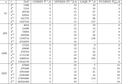
The results presented in Table1 are for the Backward Euler time-stepping method and show that for
450
all methods, iteration numbers are essentially independent of the number of time steps. Mesh independent
451
convergence is observed for MINRES and GMRES, but not for LSQR. FGMRES with the AMG
precon-452
ditioner PM G performs well for coarse discretisations, but there is some iteration growth as the mesh is 453
refined. Although this particular AMG algorithm is not accurately approximating the diagonal blocks in
454
I`⊗A0+Λ⊗A1 (cf. Section 3.1), we would expect better performance from a tailored AMG algorithm. 455
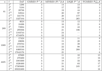
Similar results are observed for the BDF2 method (see Table 2), with iteration counts for GMRES and
456
MINRES with∣P∣robust with respect to the number of time steps and mesh width.
457
We note that using the symmetrization method within MINRES results in higher iteration numbers
458
than seen when applying GMRES to the non-symmetric system. For practical purposes it may, therefore,
459
be advantageous to use GMRES even though there is then no theoretical guarantee of fast convergence. We
460
include results for both iterative methods for comparison. We also notice that whilst the LSQR method
461
has comparable iterations counts to MINRES for small values of`, for larger numbers of time-steps LSQR
462
requires a significant increase in iterations.
[image:13.612.104.511.414.696.2]463
Table 1: Iteration numbers for the heat equation using the Backward Euler method. (— indicates iterations above the maximum of 300 or that GMRES stagnated.)
n ` DoF GMRESP−1A
MINRES∣P∣−1YA
LSQRP−1A
FGMRESP−1 MGA
81
24 1296 3 12 10 3
26 5184 3 13 16 3
28 20736 3 15 27 3
210 82944 3 15 52 3
212 331776 3 15 90 3
214 1327104 3 14 157 3
289
24 4624 3 11 10 8
26 18496 3 13 14 8
28 73984 3 15 27 8
210 295936 3 19 56 8
212 1183744 3 18 130 7
214 4734976 3 16 — 7
1089
24 17424 3 10 9 8
26 69696 3 13 13 8
28 278784 3 14 24 8
210 1115136 3 18 50 8
212 4460544 3 20 128 7
214 17842176 3 19 — 6
4225
24 67600 3 10 7 15
26 270400 3 11 12 16
28 1081600 3 13 21 16
210 4326400 3 18 44 16
212 17305600 3 20 113 17
214 69222400 2 19 — 16
Table 2: Iteration numbers for the heat equation using the BDF2 method. (— indicates iterations above the maximum of 300 or that GMRES stagnated.)
n ` DoF GMRESP−1A
MINRES∣P∣−1YA
LSQRP−1A
FGMRESP−1 MGA
81
24 1296 3 14 13 3
26 5184 3 17 22 3
28 20736 3 19 44 3
210 82944 3 20 97 3
212 331776 3 20 177 3
214 1327104 3 18 265 3
289
24 4624 3 13 12 7
26 18496 3 16 21 8
28 73984 3 19 43 8
210 295936 3 21 106 7
212 1183744 3 24 — 7
214 4734976 3 22 — 6
1089
24 17424 3 13 11 8
26 69696 3 15 20 8
28 278784 3 18 39 8
210 1115136 3 22 98 7
212 4460544 3 24 288 7
214 17842176 3 25 — 6
4225
24 67600 3 11 10 15
26 270400 3 13 17 16
28 1081600 3 18 33 16
210 4326400 3 21 83 17
212 17305600 3 24 245 17
214 69222400 3 25 — 16
6.2. Convection diffusion equation. The convection diffusion test problem is given by Example 6.1.4
464
in [10] and is known as the double glazing problem. The wind is described byw= (2y(1−x2),−2x(1−y2)).
465
Dirichlet boundary conditions are imposed everywhere on the boundary, withu=1 on the boundary where
466
x=1 and zero on all other boundaries. The initial vector u0 was zero everywhere except the boundaries 467
where it satisfies the boundary conditions. Streamline-Upwind Petrov Galerkin (SUPG) stabilization [3] was
468
used to stabilize the system. For this problem we used Backward Euler time-stepping with time-step size
469
τ=1/`.
470
As this is a non-symmetric system and the spatial operators do not commute, we were not able to use
471
the simultaneous diagonalization method described in Section3.1.1. However, we were still able to apply the
472
absolute value preconditioner, although this did require computing`diagonalizations. We therefore also used
473
the AGMG preconditioner with both the FGMRES and BiCGSTAB methods. For the exact preconditioner,
474
we used the backslash operator in Matlab i.e. an elimination (direct) method was used for the relevant block
475
systems.
476
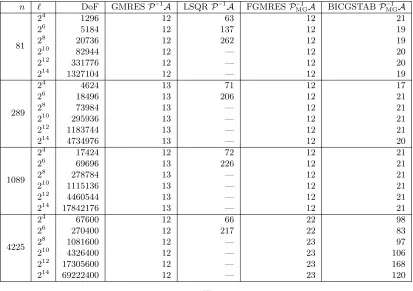
We can see iteration numbers for GMRES that are independent of the number of time-steps and
essen-477
tially also independent of the grid size. The results for FGMRES and BiCGSTAB with the AMG
precon-478
ditioner show similar trends; though the iteration counts increase for the largest spatial grid, this method
479
allows solution of these problems for all numbers of time steps. As for the heat equation, we could expect
480
more robust performance from an AMG algorithm better suited to our problem. For the LSQR method,
481
although we are able to prove that the number of non-unit eigenvalues of the normal equations is
indepen-482
dent of`the values taken by the outlying eigenvalues can become large as `increases; we therefore see that
483
the number of LSQR iterations grows quite rapidly and so this method is unlikely to be practical. There is
484
essentially no growth in the number of iterations for the GMRES, FMGRES and BiCGSTAB methods to
485
which our analysis does not apply, with the exception of the the finest grid for which the AMG component
486
of the preconditioner seems less effective.
[image:15.612.100.513.424.715.2]487
Table 3: Iteration numbers for the convection diffusion equation (- indicates iterations above the maximum of 300).
n ` DoF GMRESP−1A
LSQRP−1A
FGMRESP−1
MGA BICGSTABP
−1 MGA
81
24 1296 12 63 12 21
26 5184 12 137 12 19
28 20736 12 262 12 19
210 82944 12 — 12 20
212 331776 12 — 12 20
214 1327104 12 — 12 19
289
24 4624 13 71 12 17
26 18496 13 206 12 21
28 73984 13 — 12 21
210 295936 13 — 12 21
212 1183744 13 — 12 21
214 4734976 13 — 12 20
1089
24 17424 12 72 12 21
26 69696 13 226 12 21
28 278784 13 — 12 21
210 1115136 13 — 12 21
212 4460544 13 — 12 21
214 17842176 13 — 12 21
4225
24 67600 12 66 22 98
26 270400 12 217 22 83
28 1081600 12 — 23 97
210 4326400 12 — 23 106
212 17305600 12 — 23 168
214 69222400 12 — 23 120
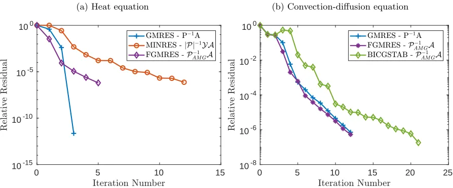
In order to further investigate the convergence properties of the proposed methods in practice, in Figure3 488
we have plotted the convergence curves for each, with the exception of LSQR for which convergence was
489
significantly slower. For the heat equation, we see that GMRES with the exact preconditioner exhibits
490
rapid residual norm reduction at the third iteration while the other methods converge at comparable rates.
491
For convection-diffusion, we do not see this drop off in the GMRES convergence curve with the exact
492
preconditioner. This is likely due to the small number of distinct eigenvalues for the preconditioned system
493
for the heat equation as compared with the convection-diffusion equation. We see that BiCGSTAB behaves
494
differently to GMRES however there is no associated theory for convergence of the preconditioner with this
495
method. Note as well that, since BiCGSTAB requires two matrix-vector products and two preconditioner
496
solves at each iteration, its cost per iteration is roughly double that of GMRES and MINRES. All methods
497
converge fairly well in these computations, but the theory only guarantees this for MINRES.
498
Fig. 3: Convergence of each of the methods (n=1089,`=210).
(a) Heat equation
0 5 10 15
10-15 10-10 10-5 100
(b) Convection-diffusion equation
0 5 10 15 20 25
10-8 10-6 10-4 10-2 100
When calculating the solution of a time-dependent problem in a sequential manner, an error at a given
499
time-step is typically propagated forward at subsequent time-steps. As the all-at-once method computes the
500
solution at all time-steps simultaneously, the error in the solution at each individual time-step may have a
501
different distribution than when calculated sequentially.
502
Figure4shows the residual of the linear system at each time-step when calculated by each method. For
503
the sequential methods, the LU factorization of the matrix in (2) was calculated and then used to evaluate the
504
solution at each step. We also note that this method has essentially solved the problem to machine precision,
505
although the error grows slightly at later time-steps. For the heat equation, the all-at-once GMRES methods
506
have essentially constant residuals after the first time step. Interestingly, for the heat equation, the residuals
507
for the symmetrized MINRES method are symmetric over the time interval i.e. the residual atti=iτ equals 508
the residual at t`−i+1 = (`−i+1)τ. However, this is not replicated for the convection-diffusion problem. 509
Again note that BiCGStab requires roughly twice the work per iteration of GMRES and MINRES.
510
7. Conclusions. We have presented a method of preconditioning an all-at-once system of evolutionary
511
equations with constant time-steps based on circulant methods for Toeplitz matrices. For symmetric systems,
512
such as the heat equation, on a regular grid we can use simultaneous diagonalization to efficiently apply a
513
block circulant or its absolute value as a preconditioner. We can also rewrite the system as a symmetric
514
one through the use of a block Hankel matrix. This allows us to use MINRES and to provide an eigenvalue
515
analysis, which guarantees convergence in a maximum number of iterations independent of the number
516
of time-steps. In practice we observe much better convergence even than predicted by this eigenvalue
517
analysis. For non-symmetric systems, we can also provide eigenvalue analysis for the preconditioned normal
518
equations. For both symmetric and non-symmetric systems an algebraic multigrid process can also be
519
[image:16.612.81.528.254.440.2]Fig. 4: Residual of the solution at each time-step (n=1089,`=210).
(a) Heat equation
200 400 600 800 1000
10-15 10-10 10-5 100
(b) Convection-diffusion equation
200 400 600 800 1000
10-15 10-10 10-5 100
employed to approximate the preconditioner; this provides an inexpensive alternative. Although we cannot
520
prove convergence bounds when AMG is used in this way, we nevertheless see promising results for both
521
symmetric and non-symmetric spatial operators with our approach. Due to the block diagonal structures
522
present in the application of the preconditioners, we believe that parallel-in-time implementations may be
523
possible however investigation of this would require further research.
524
REFERENCES 525
[1] A. O. H. Axelsson and J. G. Verwer,Boundary value techniques for initial value problems in ordinary differential 526
equations, Math. Comp., 45 (1985), pp. 153–171. 527
[2] J. H. Brandts and R. Reiss da Silva,Computable eigenvalue bounds for rank-kperturbations, Linear Algebra Appl., 528
432 (2010), pp. 3100–3116. 529
[3] A. N. Brooks and T. J. Hughes,Streamline upwind/Petrov-Galerkin formulation for convection dominated flows with
530
particular emphasis on the incompressible Navier-Stokes equations, Comput. Methods Appl. Mech. Engrg., 32 (1982), 531
pp. 199–259. 532
[4] J. R. Cardoso and F. S. Leite, Exponentials of skew-symmetric matrices and logarithms of orthogonal matrices, J. 533
Comput. Appl. Math., 233 (2010), pp. 2867–2875. 534
[5] R. H.-F. Chan and X.-Q. Jin,An Introduction to Iterative Toeplitz Solvers, SIAM, Philadelphia, PA, USA, 2007. 535
[6] T. Chan,An optimal circulant preconditioner for Toeplitz systems, SIAM J. Sci. Statist. Comput., 9 (1988), pp. 766–771. 536
[7] A. J. Christlieb, C. B. Macdonald, and B. W. Ong,Parallel high-order integrators, SIAM J. Sci. Comput., 32 (2010), 537
pp. 818–835,doi:10.1137/09075740X. 538
[8] H. Elman, A. Ramage, and D. Silvester,Algorithm 866: IFISS, a Matlab toolbox for modelling incompressible flow, 539
ACM Trans. Math. Software, 33 (2007), pp. 2–14. 540
[9] H. Elman, A. Ramage, and D. Silvester, IFISS: A computational laboratory for investigating incompressible flow 541
problems, SIAM Rev., 56 (2014), pp. 261–273. 542
[10] H. Elman, D. J. Silvester, and A. J. Wathen,Finite elements and fast iterative solvers: with applications in
incom-543
pressible fluid dynamics, Numerical Mathematics and Scientific Computation, Oxford University Press, Oxford, UK, 544
2nd ed., 2014. 545
[11] M. Emmett and M. L. Minion,Toward an efficient parallel in time method for partial differential equations, Commun. 546
Appl. Math. Comput. Sci., 7 (2012), pp. 105–132,10.2140/camcos.2012.7.105. 547
[12] R. D. Falgout, S. Friedhoff, T. V. Kolev, S. P. MacLachlan, and J. B. Schroder,Parallel time integration with
548
multigrid, SIAM J. Sci. Comput., 36 (2014), pp. C635–C661,doi:10.1137/130944230. 549
[13] D. C.-L. Fong and M. Saunders,LSMR: An iterative algorithm for sparse least-squares problems, SIAM J. Sci. Comput., 550
33 (2011), pp. 2950–2971. 551
[14] M. J. Gander,50 years of time parallel time integration, in Multiple Shooting and Time Domain Decomposition Methods, 552
T. Carraro, M. Geiger, S. K¨orkel, and R. Rannacher, eds., Springer International Publishing, Switzerland, 2015, 553
pp. 69–113. 554
[15] M. J. Gander, L. Halpern, J. Ryan, and T. T. B. Tran,A Direct Solver for Time Parallelization, Springer International 555
Publishing, 2016, pp. 491–499. 556
[16] M. J. Gander and M. Neum¨uller,Analysis of a new space-time parallel multigrid algorithm for parabolic problems, 557
SIAM J. Sci. Comput., 38 (2016), pp. A2173–A2208,doi:10.1137/15M1046605. 558
[17] M. J. Gander and S. Vandewalle,Analysis of the parareal time-parallel time-integration method, SIAM J. Sci. Comput., 559
29 (2007), pp. 556–578,doi:10.1137/05064607X. 560
[18] A. Greenbaum, V. Pt`ak, and Z. Strakoˇs, Any nonincreasing convergence curve is possible for GMRES, SIAM J. 561
Matrix Anal. Appl., 17 (1996), pp. 465–469. 562
[19] S. G¨uttel,A parallel overlapping time-domain decomposition method for odes, in Domain decomposition methods in 563
science and engineering XX, vol. 91 of Lect. Notes Comput. Sci. Eng., Springer, Heidelberg, 2013. 564
[20] W. Hackbusch, Parabolic multi-grid methods, in Proceedings of the Sixth International Symposium on Computing 565
Methods in Applied Sciences and Engineering, VI, R. Glowinski and J.-L. Lions, eds., North-Holland, Amsterdam, 566
1984, pp. 189–197. 567
[21] L. Hemmingsson, A semi-circulant preconditioner for the convection-diffusion equation, Numer. Math., 81 (1998), 568
pp. 211–248,doi:10.1007/s002110050390. 569
[22] M. R. Hestenes and E. Stiefel,Methods of conjugate gradients for solving linear systems, J. Res. Nat. Bur. Stand., 49 570
(1952), pp. 409–435,nvl.nist.gov/pub/nistpubs/jres/049/6/V49.N06.A08.pdf. 571
[23] G. Horton and S. Vandewalle,A space-time multigrid method for parabolic partial differential equations, SIAM J. Sci. 572
Comput., 16 (1995), pp. 848–864,doi:10.1137/0916050. 573
[24] T. K. Huckle and D. Noutsos, Preconditioning block Toeplitz matrices, Electron. Trans. Numer. Anal., 29 (2007), 574
pp. 31–45. 575
[25] D. Lahaye, H. De Gersem, S. Vandewalle, and K. Hameyer,Algebraic multigrid for complex symmetric systems, 576
IEEE Trans. Magn., 36 (2000), pp. 1535–1538. 577
[26] J.-L. Lions, Y. Maday, and G. Turinici,A parareal in time discretization of PDEs, C.R. Acad. Sci. Paris, Serie I, 332 578
(2001), pp. 661–668,doi:10.1016/S0764-4442(00)01793-6. 579
[27] S. MacLachlan and C. Oosterlee,Algebraic multigrid solvers for complex-valued matrices, SIAM J. Sci. Comp., 30 580
(2008), pp. 1548–1571. 581
[28] Y. Maday and E. M. Rønquist,Parallelization in time through tensor-product space–time solvers, Comptes Rendus 582
Mathematique, 346 (2008), pp. 113–118. 583
[29] W. L. Miranker and W. Liniger, Parallel methods for the numerical integration of ordinary differential equations, 584
Math. Comp., 21 (1967), pp. 303–320. 585
[30] A. Napov and Y. Notay,Aggregation-based algebraic multigrid for convection-diffusion equations, SIAM J. Sci. Comput., 586
34 (2012), pp. A2288–A2316. 587
[31] A. Napov and Y. Notay,An algebraic multigrid method with guaranteed convergence rate, SIAM J. Sci. Comput., 34 588
(2012), pp. A1079–A1109. 589
[32] M. K. Ng,Iterative Methods for Toeplitz Systems, Oxford University Press, Oxford, UK, 2004. 590
[33] Y. Notay,AGMG software and documentation; see http://homepages.ulb.ac.be/ ynotay/AGMG. 591
[34] Y. Notay,An aggregation-based algebraic multigrid method, Electron. Trans. Numer. Anal., 37 (2010), pp. 123–146. 592
[35] J. A. Olkin,Linear and nonlinear deconvolution problems, PhD thesis, Rice University, 1986. 593
[36] I. Oseledets and E. Tyrtyshnikov,A unifying approach to the construction of circulant preconditioners, Linear Algebra 594
Appl., 418 (2006), pp. 435–449,doi:10.1016/j.laa.2006.02.037. 595
[37] C. Paige and M. Saunders,Solution of sparse indefinite systems of linear equations, SIAM J. Numer. Anal, 12 (1975), 596
pp. 617–629. 597
[38] C. C. Paige and M. A. Saunders,LSQR: An algorithm for sparse linear equations and sparse least squares, ACM Trans. 598
Math. Software, 8 (1982), pp. 43–71,doi:10.1145/355984.355989. 599
[39] B. Parlett,The symmetric eigenvalue problem, SIAM, Philadelphia, PA, USA, classics ed., 1998. 600
[40] J. Pestana and A. J. Wathen,A preconditioned MINRES method for nonsymmetric Toeplitz matrices, SIAM J. Matrix 601
Anal. Appl., 36 (2015), pp. 273–288. 602
[41] S. Reitzinger, U. Schreiber, and U. van Rienen,Algebraic multigrid for complex symmetric matrices and applications, 603
J. Comput. Appl. Math., 155 (2003), pp. 405–421. 604
[42] D. Sheen, I. Sloan, and V. Thom´ee,A parallel method for time discretization of parabolic equations based on Laplace
605
transformation and quadrature, IMA J. Numer. Anal., 23 (2003), pp. 269–299. 606
[43] D. Silvester, H. Elman, and A. Ramage,Incompressible Flow and Iterative Solver Software (IFISS) version 3.2, May 607
2012.http://www.manchester.ac.uk/ifiss/. 608
[44] G. Strang,A proposal for Toeplitz matrix calculations, Stud. Appl. Math., 74 (1986), pp. 171–176. 609
[45] C. Van Loan,Compuational Frameworks for the Fast Fourier Transform, SIAM, Philadelphia, PA, USA, 1992. 610
[46] E. Vecharynski and A. V. Knyazev,Absolute value preconditioning for symmetric indefinite linear systems, SIAM J. 611
Sci. Comput., 35 (2013), pp. A696–A718. 612
[47] A. J. Wathen,Preconditioning, Acta Numer., 24 (2015), pp. 329–376,doi:10.1017/S0962492915000021. 613