Improved very-short-term wind forecasting using atmospheric regimes

DOI: 10.1002/we.2207

R E S E A R C H A R T I C L E

Improved very short-term spatio-temporal wind forecasting

using atmospheric regimes

J. Browell

D. R. Drew

K. Philippopoulos

1_{Department of Electronic and Electrical}

Engineering, University of Strathclyde, Glasgow, UK

2_{Department of Meteorology, University of}

Reading, Reading, UK

Correspondence

J. Browell, Technology and Innovation Centre, University of Strathclyde, 99 George Street, Glasgow G1 1RD, UK.

Email: jethro.browell@strath.ac.uk

Funding information

University of Strathclyde's EPSRC Doctoral Prize, Grant/Award Number: EP/M508159/1; NERC NPIF fellowship, Grant/Award Number: NE/RE013276/1

Abstract

We present a regime-switching vector autoregressive method for very short-term wind speed

forecasting at multiple locations with regimes based on large-scale meteorological phenomena.

Statistical methods for wind speed forecasting based on recent observations outperform

numer-ical weather prediction for forecast horizons up to a few hours, and the spatio-temporal

inter-dependency between geographically dispersed locations may be exploited to improve forecast

skill. Here, we show that conditioning spatio-temporal interdependency on “atmospheric modes”

derived from gridded numerical weather data can further improve forecast performance.

Atmo-spheric modes are based on the clustering of surface wind and sea-level pressure fields, and the

geopotential height field at the 5000-hPa level. The data fields are extracted from the MERRA-2

reanalysis dataset with an hourly temporal resolution over the UK; atmospheric patterns are

clus-tered using self-organising maps and then grouped further to optimise forecast performance. In a

case study based on 6 years of measurements from 23 weather stations in the UK, a set of 3

atmo-spheric modes are found to be optimal for forecast performance. The skill of 1- to 6-hour-ahead

forecasts is improved at all sites compared with persistence and competitive benchmarks. Across

the 23 test sites, 1-hour-ahead root mean squared error is reduced by between 0.3% and 4.1%

compared with the best performing benchmark and by an average of 1.6% over all sites; the

6-hour-ahead accuracy is improved by an average of 3.1%.

KEYWORDS

atmospheric classification, forecasting, vector autoregression, wind speed

1

INTRODUCTION

Wind energy is providing a significant and increasing share of electricity generation in power systems around the world, and this trend is expected

to continue in light of global commitments to decarbonise society.1_{Operating power systems and participating in electricity markets with high}

penetrations of wind energy demands continuous improvement in wind power forecasting to reduce the negative impact of forecast errors and

uncertainty on operational costs and reliability.2,3_{Atmospheric conditions have a significant bearing on forecast performance, and codifying this is an}

active area of research. For example, cyclone detection has been used to predict periods of potentially large forecast error in day-ahead wind power

forecasting.4_{Here, we are concerned with very short-term forecasts of the order of minutes to hours ahead which are of particular importance to}

participants in intraday markets and the balancing function of power system operators.2,5

On these time scales, statistical methods based on time series analysis are generally superior to those based on post-processing numerical

weather predictions due to the easy assimilation of new measurements and low computational cost of producing new forecasts.6_{Many time series}

methods have been used for wind speed (WS) and power forecasting including autoregressive (AR)7_{and autoregressive moving average (ARMA)}8

and various machine learning methods including neural networks9_{and Markov chains.}10,11_{Hybrid methods that combine multiple prediction layers}

or blend forecasts from multiple methods have also been studied and shown to outperform individual methods in some cases.12

. . . .

This is an open access article under the terms of the Creative Commons Attribution License, which permits use, distribution and reproduction in any medium, provided the original work is properly cited.

© 2018 The Authors Wind Energy Published by John Wiley & Sons Ltd.

Information from spatially distributed measurements can be used to model spatio-temporal dependency and thereby improve forecast skill at all

measurement locations.13,14_{Measurements from multiple locations are typically embedded in a single vector, and the temporal evolution of that}

vector is modelled in a vector autoregressive (VAR) framework. An exposition of VAR modelling is available in Lütkepohl.15_{Furthermore, the spatial}

dependency structure may itself depend on externalities such as season or wind direction.16,17_{However, the number of parameters to be estimated}

scales with the square of the number of spatial locations making these methods impractical for large problems. More recently, advances have been

made in sparse parameter estimation in order to make large-scale problems, those dealing with hundreds or potentially thousands of locations,

tractable.18,19

In parallel to the development of spatial models, forecasting schemes based on multiple models designed for specific conditions orregimeshave

been proposed. Regime-switching methods have been applied to forecast offshore wind power fluctuations in Pinson et al,20_{and WS in Ailliot and}

Monbet,21_{where the regime-switching process is “unobserved” and modelled as a hidden Markov process. In the first case, the number of regimes}

is chosen to be 3 by expert judgement to reflect the 3 distinct regions of the wind farm power curve, and in the second case by numerical experiment.

An adaptive extension to this approach is presented in Pinson and Madsen.22_{The 2017 EEM Wind Power Forecasting Competition was won with a}

regime-switching AR method23_{using regimes defined on exogenous variables. Specifically, regimes were identified by clustering the previous day's}

zonal and meridional WS measurements, and separate AR models were produced for each regime. Defining regimes by some exogenous variable,

or variables, enables forecasters to explicitly incorporate information associated with physical processes that are relevant to the forecasting task.

Furthermore, doing so separately from the estimation of forecast model parameters avoids the need for the computationally expensive procedures

required to fit hidden Markov models, which estimate the parameters of both the regime-switching process and AR model iteratively, with or without

exogenous variables.

A spatio-temporal regime-switching model for WS prediction is proposed in Gneiting et al13_{with 2 regimes based on wind direction. Large-scale}

pressure differences that result in either easterly or westerly winds being channelled through the Columbia Gorge define the regimes, and regimes

are switched between based on recent observations of wind direction for forecasting. A more general approach is developed in Hering et al24_and

Kazor and Hering25_{by fitting a mixture of bivariate normal distributions to the wind vector, which may be a spatial average, and defining regimes by}

the mixture components. The identification of regimes based on multiple measurement locations has been studied in Burlando et al26_{and Kazor and}

Hering.27_{However, these methods rely on only a few measurement locations relative to the scale of the meteorological phenomena that underpin}

the spatial structure in surface winds, and as a result, regime definitions depend on the exact combination of sites under consideration. In this work,

we aim to decouple the identification of weather regimes from the geographic distribution of measurement locations by identifying weather regimes

for a large region using a grid of numerical weather predictions.

For a given region, there may be a wide range of possible large-scale meteorological conditions due to variations in the strength and location

of synoptic-scale weather features, defined as atmospheric motion with a typical spatial scale of many hundreds of kilometres, such as

extratrop-ical cyclones or high-pressure systems.28,29_{Unsupervised learning, or clustering, techniques may be used to codify these large-scale atmospheric}

circulation patterns in terms of a relatively small number of distinct modes30,31_{defined based on the fields of mean sea-level pressure (SLP) and}

geopotential height, for example, for each time instant of interest. To reduce the number of modes for specific applications, a second clustering stage

may be applied, akin to Weia and Mohanb32_{and Ohba et al.}33_{In the meteorological literature, this process is sometimes referred to as}

“classifi-cation,” but we avoid the use of that term here as in broader usage, this term implies a form of supervised learning. Given the length scale of the

synoptic-scale features, modes are typically determined on a daily temporal resolution; however, the same methods can be used to cluster patterns

on any temporal scale from subdaily to seasonal depending on the application. In the very short-term setting here, we issue forecasts every hour on

a rolling basis and therefore also consider atmospheric modes at hourly resolution.

In this paper, we introduce a conditional regime-switching VAR model with regimes conditioned on atmospheric modes defined by a 2-stage

clus-tering method. In sections 2.1 to 2.3, the univariate AR model is introduced and extended to the proposed conditional VAR model. The identification

of atmospheric modes via self-organising maps is described in 2.4. A UK-based case study comprising 6 years of measurement data is introduced in

Section 3, and results are presented in Section 4. Finally, conclusions are drawn and discussed in Section 5.

2

FORECASTING FRAMEWORK

Consider a WS time series denotedY= {y1,y2,…,yT}. We aim to forecastyt+𝜏at timetand in order to do so find some functionf𝜏(·)that maps a vector explanatory variablesxtontoyt+𝜏,

̂

yt+𝜏|t=f𝜏(xt), (1)

while minimising some function of the prediction error, which is given byet+𝜏|t=ŷt+𝜏|t−yt+𝜏.

2.1

Autoregression

For time series that exhibit serial correlation, such as WS measurements, it is reasonable for the vector of explanatory variables to consist of the

recent history ofyt,

̂

yt+𝜏|t=f𝜏(yt,yt−1,yt−2,· · ·), (2)

̂

yt+𝜏|t=𝜈𝜏+ p−1

∑

i=0

𝛼i,𝜏yt−i. (3)

This is the familiar AR model of orderp, denoted AR(p). The choice of the model orderpand estimation of parameters𝜈𝜏, 𝛼i,𝜏,i= 0,…,p−1will be discussed in the next section. In the remainder of this section, a number of extensions to the AR(p) model relevant to WS forecasting are introduced.

A natural extension of the AR model is the inclusion of exogenous explanatory variables, such models are sometimes denoted “ARX.” Since WS

exhibits diurnal seasonality, the time of day is included as a set of dummy variables, denoteddh(t),h∈, whereis the set of discrete measurement times appropriate to the temporal resolution of the data, eg,= {0,1,· · ·,23}in the case of hourly measurements, and

dh(t) = {

1 if Hour(t) =h

0 otherwise . (4)

The AR model with exogenous variables, ARX(p), is written

̂ yt+𝜏|t=

p−1

∑

i=0

𝛼i,𝜏yt−i+ ∑

h∈

𝛽h,𝜏dh(t+𝜏), (5)

where the intercept𝜈𝜏is superseded by𝛽h,𝜏, which may be interpreted as time-dependent intercepts. Diurnal cycles may be modelled by a variety

of other approaches, notably by estimating a smooth function of the time of day and detrending the data as a form of preprocessing, as in Hill et al,14

or retaining them in anadditive model,34_{as in Ziel et al.}35_{Here, we proceed with dummy variables, as they are flexible and easily interpretable as a}

time-of-day bias correction.

Any categorical exogenous variable may be modelled in this way, and we also consider ARX models where dummy variables for the current

atmospheric modemt∈= {1,2,· · ·,M}are included with associated parameters𝛾s,𝜏. In this case, (5) becomes

̂ yt+𝜏|t=

p−1

∑

i=0

𝛼i,𝜏yt−i+ ∑

h∈

𝛽h,𝜏dh(t+𝜏) + ∑

s∈𝛾

s,𝜏1s(mt), (6)

where the indicator function₁s(mt) =1ifmt = sand 0 otherwise. The parameter𝛾s,𝜏acts as a bias correction for modesat forecast horizon𝜏. The sum𝛽h,𝜏 +𝛾s,𝜏may be interpreted as a time and atmospheric mode-dependent intercept term.

We conjecture that the dependence of the processYon atmospheric mode is more complex than the bias correction modelled by a dynamic

intercept and therefore consider switching between ARX models that are mode-specific, such that (5) becomes

̂ yt+𝜏|t=

p−1

∑

i=0

𝛼i,𝜏,m_tyt−i+ ∑

h∈

𝛽h,𝜏,m_tdh(t+𝜏), (7)

where each parameter of the ARX model depends the atmospheric modemtat the forecast issue time.

2.2

Vector autoregression

It is advantageous to consider multiple locations simultaneously in order to capture interdependency among lagged measurements for spatially

dispersed sites. This is achieved by extending the AR time-series models described above to VAR models. Measurements made at timetand atN

locations are embedded in the vectoryt∈RN, and we consider the vector-valued time seriesY = {y1,y2,…,yT}. The basic VAR(p) process is the “vectorised” form of (3) and is written

̂

yt+𝜏|t= p−1

∑

i=0

Ai,𝜏yt−i, (8)

whereAi,𝜏∈RN×Nare matrices of parameters. This model is used as a benchmark in the proceeding study and is referred to asVAR. Parameters on the diagonal ofAi,𝜏capture autocorrelation effects and off-diagonal parameters capture cross-correlation. Exogenous variables may be incorporated

along similar lines give

̂

yt+𝜏|t= p−1

∑

i=0

Ai,𝜏yt−i+ ∑

h∈

𝜷h,𝜏dh(t+𝜏), (9)

with the effect of diurnal dummies parametrised by the vector𝜷h,𝜏∈RN. Throughout this paper, this model will be referred to asVAR_d. The further addition of atmospheric mode dummies parametrised by_𝜸s,𝜏∈RN, with thenth element corresponding to a bias correction for modesat siten, gives

̂

yt+𝜏|t= p−1

∑

i=0

Ai,𝜏yt−i+ ∑

h∈

𝜷h,𝜏dh(t+𝜏) + ∑

s∈

𝜸s,𝜏1s(mt), (10)

referred to asVAR_d_m. Finally, the model parameters may themselves be dependent on atmospheric mode resulting in a conditional VAR model,

referred to asCVAR_d,

̂

yt+𝜏|t= p−1

∑

i=0

Ai,𝜏,mtyt−i+ ∑

h∈

2.3

Parameter estimation

The model parametersB_𝜏,s = [

A1,𝜏,s · · · Ap,𝜏,s 𝜷0,𝜏,s · · · 𝜷23,𝜏,s ]

are estimated by minimising some function of the prediction errors on a static

dataset. It is useful to define the input data matricesX_𝜏,sand target data matricesY𝜏,sfor forecast horizon𝜏and atmospheric modes. The input data

matrices, sometimes called design matrices, are the vertical concatenation of explanatory variables for which corresponding target variables are

known and are written

X_𝜏,s= ⎡ ⎢ ⎢ ⎢ ⎣ ⋮ ⋮ ⋮ ⋮ yT

i · · · y

T

i−p+1 d0(i+𝜏) · · · d23(i+𝜏)

⋮ ⋮ ⋮ ⋮ ⎤ ⎥ ⎥ ⎥ ⎦ (12)

for1_≤i_<T−𝜏subject tomi = s. The corresponding matrix of target data is the vertical concatenation of WS vectors given by

Y_𝜏,s= ⎡ ⎢ ⎢ ⎢ ⎣ ⋮ yT i ⋮ ⎤ ⎥ ⎥ ⎥ ⎦ (13)

forp+𝜏 ≤i_≤Tsubject tomi−𝜏 = s. The matrix of prediction errors for all sites and times in the dataset corresponding to modeswith forecast horizon𝜏is given byE𝜏,s=Y𝜏,s−X𝜏,sBT𝜏,s. The parameter matrixB𝜏,smay now be estimated by minimising an appropriate function ofE𝜏,s.

Ordinary least squares (OLS) is used here for simplicity though different cost functions may be more appropriate for specific forecasting tasks,

such as the quantile loss function for nonparametric probabilistic forecasting. The OLS parameters estimates are the solution to

argmin B_𝜏,s

||E𝜏,s||22=argmin

B_𝜏,s ‖‖

‖Y𝜏,s−X𝜏,sBT𝜏,s‖‖_‖

2

2, (14)

which is popular due to its simple solution by differentiation given by

̂

B_𝜏,s= (

XT

𝜏,sX𝜏,s )−1

XT

𝜏,sY𝜏,s. (15)

The OLS parameter estimate is equal to the maximum likelihood estimate in the special case that the rows ofE_𝜏,sare independent and identically

distributed and follow a multivariate normal distribution with zero mean and covariance matrix of the form_𝜎2

𝜏,sI. The number of samples available for parameters estimation is an important consideration, as insufficient training data will result in noisy parameter estimates.15_{As the parameters}

of the conditional VAR are estimated using only a subset of the available training data corresponding to a specific mode, the size of each subset may

become a factor in the quality of the parameter estimates if a large number of atmospheric modes is considered or if there is only a small amount of

training data available for 1 or more modes.

2.4

Atmospheric clustering

The proposed forecasting methodology uses the large-scale atmospheric situation as an exogenous explanatory variable based on clustering

numer-ical weather prediction data toMdistinct atmospheric regimes. There are a wide variety of methodologies available to cluster circulation patterns.

These can be divided into 3 categories as proposed in Huth et al30_{: subjective (manual), mixed (hybrid), and objective (automated). In this study, a}

2-stage automated clustering approach is adopted, where thek-means algorithm is applied to further group the atmospheric patterns identified in

“Understanding the wind energy production variability in Great Britain – A synoptic climatology using Self-Organizing Maps.”36_{A mixed approach}

is also considered whereby the second-stage grouping is made by expert judgement.

The self-organising map (SOM) is a 2-layer artificial neural network consisting of an input layer and an output 2-dimensional lattice of neurons,

characterized by their synaptic weights vector,w, and their location at the SOM lattice. Learning in SOM is achieved through the processes of

com-petition, cooperation, and adaptation. During the competition phase, an input pattern is presented to the SOM, and a metric distance is calculated

for all neurons. The neuron with the smallest distance is the “winner” orbest matching unit(BMU), and a radial basis function centred on the BMU

determines the topological neighbourhood of “excited” neurons in the SOM lattice during the cooperation phase. Finally, in the adaptation phase

the BMU and the excited neurons' weight vectors are updated towards the input vector.

To describe the atmospheric circulation with a higher degree of generalisation, ak-means clustering algorithm is performed as a post-processing

step for further grouping the SOM patterns. Thek-means algorithm defines centroids through an iterative procedure and then assigns input data

to the nearest centroid. It has been applied to group atmospheric patterns produced by SOMs in other works, such as Weia and Mohanb,32_Ohba

et al,33_{and Vesanto and Alhoniemi}37_{and is chosen here for its computational efficiency and interpretability. Here, we are only interested in “hard”}

assignments of observations to clusters, in contrast to probabilistic methods which make “soft” assignments based on the probability of belonging

to each mixture component, such as Gaussian mixture models. However, we note that the EM algorithm for estimating Gaussian mixture models

reduces to thek-means algorithm in the limit of hard assignments; for details, see Bishop.38_{The atmospheric fields considered are approximately}

Gaussian but have variances of different orders of magnitude, so they are standardised prior to clustering. Thek-means algorithm is similar to the

SOM learning process only without cooperation and adaptation phases. For comparison, a subjective approach is tested whereby the SOM patterns

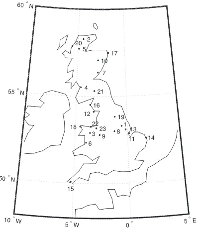
FIGURE 1 Locations of the 23 weather stations supplying data to the Met Office Integrated Data Archive System considered in this study. Measurements of hourly mean wind speed measured at 10m above ground covering years from 2002 to 2007 are used

3

CASE STUDY

The proposed conditional VAR model and benchmarks are tested on measurements of hourly mean WS made in the UK at 23 weather stations

(shown in Figure 1) from 2002 to 2007. These data were extracted from the Met Office Integrated Data Archive System via the British Atmospheric

Data Centre.39_{Hourly mean WS measured at 10 m above ground is used in this study. These sites all have greater than 98% “good” data coverage}

following quality control by the British Atmospheric Data Centre. Years 2002 to 2005 are used for model order selection via tenfold cross-validation,

and 2006 to 2007 are used for out-of-sample testing. Forecasts are produced for 1 to 6 hours ahead for all locations, meaning that in total, over 2.41

million out-of-sample forecasts have been produced and evaluated in this study. Throughout the analysis, the performance of proposed conditional

VAR model (CVAR_d) is benchmarked against a range of other models outlined in Equations 8 to 10, including persistence, VAR, VAR with diurnal

dummies (VAR_d), and VAR with diurnal and atmospheric mode dummies (VAR_d_m).

3.1

Atmospheric clustering

The SOM implementation used here is based on a 4-step SOM clustering framework proposed in Philippopoulos and Deligiorgi,31_{which has}

also been applied in a climatological context over Greece to examine the relationship of wintertime meteorological conditions with atmospheric

circulation.29_{In Philippopoulos et al,}36_{the above framework is used to examine the association of atmospheric patterns with extreme wind power}

events in the UK. This approach to identifying atmospheric modes is distinct from previous work in that the surface WS field is incorporated, as a

critical input for wind energy applications, in addition to more typical large-scale variables mean SLP and geopotential height at 500hPa (Z500).

Despite WS and SLP being highly correlated, this results in the identification of a greater number of distinct atmospheric modes. The selected

vari-ables are extracted from modern-era retrospective analysis for Research and Applications Version 2 (MERRA-2) with an hourly temporal resolution

from 1980 to 2014 (34 years) and for a domain centred over the UK (from24.75◦W to15.00◦E and40.50◦N to69.75◦N) with a0.65◦×0.5◦ spa-tial resolution bilinear interpolated to a0_.75◦×0_.75◦grid. Upon the definition of the spatial and temporal scales (step 1), the spatio-temporal time series are standardised, and the principal components analysis is used as a preprocessing step for data reduction purposes (step 2). The clustering is

performed by using the SOM algorithm on the first PC scores that explain more than 1 predefined percent of the initial variance, while the optimum

size of the SOM feature map (the number of atmospheric patterns) is determined using qualitative criteria and the Davies-Bouldin index40_{(step 3).}

The resulting catalogue of atmospheric circulation patterns may then be visualised and studied as per the user's application. The application here is

to condition VAR models on atmospheric modes, and that is the focus of the remainder of this paper; for more detail on the the SOM process, please

see Philippopoulos et al.29,31,36

Multiple SOM configurations for the UK were examined in Philippopoulos et al,36_{and the optimum size of the SOM feature map contained 21}

atmospheric modes organised in a7×3hexagonal map, visualised in Figure 2. Neighbouring nodes are interconnected, and each one is associated with the composites of the selected variables. An important advantage of the approach is that relative position in the SOM map is associated with

specific features, such as seasonality, location of the pressure systems, and pressure gradient along with the wind field, enabling the extraction of

valuable information regarding the evolution of atmospheric circulation. The hexagonal topology was selected to increase the degree of

FIGURE 2 Grouping of the SOM atmospheric circulation patterns and their location in the SOM map. Each hexagon represents one of the 21 atmospheric patterns identified by the SOM. Shading corresponds to membership of the 3 clusters, or modes, found to be optimal for our forecasting application [Colour figure can be viewed at wileyonlinelibrary.com]

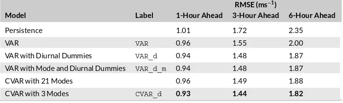
TABLE 1 Root mean squared forecast error from tenfold cross-validation on the training dataset

averaged across all locations. The lowest RMSE for each lead-time is highlighted in bold

RMSE (ms−1₎

Model Label 1-Hour Ahead 3-Hour Ahead 6-Hour Ahead

Persistence 1.01 1.72 2.35

VAR VAR 0.96 1.55 2.00

VAR with Diurnal Dummies VAR_d 0.94 1.48 1.87 VAR with Mode and Diurnal Dummies VAR_d_m 0.94 1.48 1.87

CVAR with 21 Modes 0.96 1.49 1.88

CVAR with 3 Modes CVAR_d 0.93 1.44 1.82

a_{All methods perform better than persistence across all forecast horizons, with the VAR model conditional}

on 3 atmospheric modes demonstrating the best predictive performance in each case.

cases, relatively small changes in large-scale atmospheric circulation may lead to a different surface wind field over the UK, a finding with important

implications for wind energy applications, and spatio-temporal forecasting in particular.

This study uses the hourly time series of the 21 atmospheric patterns for the period 2002 to 2007. The SOM clustering identified precisely 21

modes based on the Davies-Bouldin index, which minimises the “similarity” between clusters, but this leaves little training data available in{X_𝜏,s,Y𝜏,s }

to estimate the VAR parametersB_𝜏,s,s = 1,…,21. Furthermore, it is observed that many of the 21 modes are similar and form natural groups.

Thek-means algorithm is applied to centroids of the 21 SOM patterns in order to group the 21 atmospheric patterns intokatmospheric modes for

k = 1,…,10. In addition, 2 groupings were formed by expert judgement, one arranged the 21 patterns into 4 groups and the other into 9. The grouping used in the final forecasting model is the one with the lowest root mean squared error in a tenfold cross-validation exercise on the training

dataset.

3.2

VAR model fitting

Following model selection and estimation on the training dataset from 1/1/2002–31/12/2005, the performance of the proposed forecasting

methodology is tested on 2 years of data from 1/1/2006 to 31/12/2007. Forecasts are produced every hour on a rolling basis from 1 to 6 hours

ahead with a dedicated model for each look-ahead time.

The AR order of the VAR models (8)-(11) is chosen to bep = 3after tenfold cross-validation on the training dataset for valuesp = 1_,…,5

showed negligible difference in predictive performance, but analysis of the partial autocorrelation functions for the wind speed data for each of the

23 sites showed 3 lags to be significant in the majority of cases. While some sites showed that greater than 3 lags were significant, the results of the

cross-validation exercise did not support increasing in model complexity any further.

Summary results from the cross-validation exercise are presented in Table 1. Comparing the candidate models indicates that the conditional VAR

based on 3 atmospheric modes has the best predictive performance across forecast horizons from 1- to 6-hours ahead, showing greater

improve-ment over nonconditional methods for greater forecast horizons. The conditional VAR based on the 21 patterns from the SOM (without further

grouping) provides no improvement on the nonconditional VAR model.

3.3

Atmospheric modes and grouping

The performance of the conditional VAR model with different numbers of atmospheric modes is plotted in Figure 3. The special case of having 1

mode is equivalent to the standard nonconditional VAR and is outperformed by the conditional VAR with between 2 and 5 modes. The data-driven

FIGURE 3 Forecast performance of conditional VAR model with diurnal dummies with different groupings of atmospherics modes. Results are the product of tenfold cross-validation on the training dataset. Different methods of forming group are considered based on clustering using all variables (mean sea-level pressure, zonal and meridional wind speed components, and geopotential height at 500 hPa), and subjective judgement by expert meteorologists [Colour figure can be viewed at wileyonlinelibrary.com]

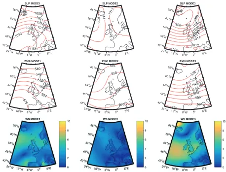
FIGURE 4 Visualisation of sea-level pressure field (SLP), geopotential height at 500 hPa (Z500), and wind speed (WS) in units of ms−1_{for the 3}

atmospheric mode centroids [Colour figure can be viewed at wileyonlinelibrary.com]

by expert judgement. It was also found that forecasts based on atmospheric modes defined using SLP and Z500 individually or combined, as is

common practice in atmospheric clustering, did not perform as well as the combination including the wind field. The forecasting error of the tenfold

cross-validation of the conditional VAR models on the training dataset increases gradually for greater than 3 modes. This can be attributed to the

degree of weather-related information required for improved wind forecasting skill without reducing the generalisation ability of the models due

to insufficient training events. Furthermore, thek-means grouping of the SOM atmospheric patterns is consistent with the inherent characteristic

at the second row of the SOM map, the second mode principally from the third row patterns, and the third mode groups all the cases from the first

row of the SOM atmospheric patterns shown in Figure 2.

The modes correspond to 3 distinct states of atmospheric circulation and wind speed conditions over the UK. The mode centroids are

illus-trated in Figure 4. Mode 1 is associated with anticyclonic circulation and moderate wind speed conditions. The high-pressure centre is located to

the south-west of UK over the Atlantic ocean, leading to an easterly component flow with maximum intensity over Scotland and northern England.

Mode 2 consists of low-wind speed cases and, indicated by the the SLP centroid, the calm conditions over the UK mainland result from the

combina-tion of the low- and high-pressure fields to the west and east, respectively. Mode 3 is directly linked with cyclonic atmospheric circulacombina-tion patterns

and relatively high wind speed conditions. The low-pressure centre can either be to the west, north, east, or over the British Isles and represents

the frequent passage of depressions over the study area. The wind direction is predominately west-south-westerly with highest wind speeds over

central and southern areas of the UK.

For the study period 2002 to 2007, the atmospheric conditions are evenly distributed across the 3 modes (32.4% of the time in mode 1, 36.0% of

the time in mode 2, and 31.6% of the time in mode 3). Both modes 1 and 2 occur throughout the year; however, there is a higher frequency of events

during the summer period, as shown in Figure 5. Approximately 40% of mode 1 events occur between May and August where the high pressure

is related to the extension of the Azores anticyclone. Similarly, approximately 50% of mode 2 events are between May and August. However, in

comparison to mode 1, mode 2 occurs less frequently during the winter months; less than 13% of events occur in between December and February.

In contrast, mode 3 is more common during the winter and transitional seasons; less than 5% of events occur between June and August. This is due

to the frequent passage of extratropical cyclones associated with the North Atlantic storm track.

The atmospheric modes are defined by synoptic-scale conditions, which have a length scale of many hundreds of kilometres and therefore tend

to persist for periods on the order of days. Figure 6 shows the cumulative frequency distribution of the duration for which each mode event persists

during the period 2002 to 2007. The distributions of modes 2 and 3 are very similar; the mean duration is 86 and 87 hours, respectively, which

equates to 3.6 days. In comparison, the duration of mode 1 is generally shorter with a mean duration of 57 hours or 2.4 days. This difference is

largely due to the higher frequency of relatively long duration events for modes 2 and 3 compared with mode 1. The median duration for mode 1, 38

FIGURE 5 Relative frequency of occurrence for each atmospheric mode by month [Colour figure can be viewed at wileyonlinelibrary.com]

FIGURE 6 Cumulative frequency distribution of the duration for which each mode event persists during the period 2002 to 2007. The duration is

hours, is actually very similar to mode 3, 42 hours; however, mode 3 is much more likely to persist for periods in excess of 10 days. This is generally

associated with the passage of consecutive extratropical cyclones, which are sufficiently close to prevent a change in the atmospheric mode. For all

3 modes, it is unusual for the duration of an event to be shorter than 6 hours (10.5% for mode 1, 8.7% for mode 2, and 8.5% for mode 3).

4

RESULTS

Conditioning the forecast on atmospheric modes increases the accuracy of the wind speed predictions across all lead times compared with the

benchmark models. For the 1-hour ahead forecast, the RMSE of the predicted wind speed averaged across the 23 sites is improved by 1.6% relative

to VAR with diurnal dummies (VAR_d) and 7.8% relative to persistence, as illustrated in in Figure 7. The improvement in the forecast skill due to the

information provided by the atmospheric modes increases with the lead time. For example, for the 6-hour ahead forecast,CVAR_dimproves the

RMSE by 3.1% relative toVAR_d, and 23.9% relative to persistence.

Figure 7 also shows the performance of the VAR model with mode and diurnal dummies (VAR_d_m) is very similar to that ofVAR_d. This indicates

the additional skill provided byCVAR_dis due to the better representation of the spatial structure of winds between the sites provided by the

atmospheric modes and that it is not simply a bias correction.

The conditional VAR modelCVAR_dproduces an improvement in the forecast at all 23 sites, illustrated in Figure 8; however, the magnitude of the

reduction in RMSE varies from site to site. For example, for the 1-hour-ahead forecasts, the reduction in RMSE varies from only 0.3% for site 11 to

4.1% for site 7. This result is also true across atmospheric modes, ie, for all sites, there is a reduction in the RMSE of the wind speed usingCVAR_d

for each of the atmospheric modes. In general,CVAR_dprovides the greatest improvement in the forecast when the atmosphere is determined to

be in mode 3, cyclonic conditions. For the 1-hour-ahead forecast, averaged across the 23 sites, there is a reduction in the RMSE of 2.4% relative to

FIGURE 7 Improvement over persistence averaged across all sites in the test dataset. The results are shown for the conditional VAR model

CVAR_d(_▵) and 3 benchmark models;VAR(_◦),VAR_d(+), andVAR_d_m(×) [Colour figure can be viewed at wileyonlinelibrary.com]

FIGURE 9 The 1-hour-ahead forecast error distribution for individual locations separated by atmospheric mode for training data (solid line) and test data (dashed line). Illustrated sites: top, Nottingham; bottom, Gorleston

VAR_dduring mode 3 events, in comparison with a reduction of 1.1% and 1.4% for modes 1 and 2, respectively. The reduction in RMSE is greatest

for mode 3 at 16 of the 23 sites. Further analysis of the sites has not revealed a clear relationship between the added value due to the atmospheric

modes and the geographical location, terrain type, or elevation of the sites.

The distributions of forecast errors are approximately symmetric about zero for all three 3 atmospheric modes and all 23 locations. Bias, the mean

forecast error, is between−0.09and 0.04 ms−1_{across all sites and modes. All but one location exhibit squared skewness below 0.01, and kurtosis}

ranges from 3.8 to 11.0. High kurtosis is indicative of a “sharper” peak than that of the normal distribution, which has a kurtosis of 3. At 13 out of 23

locations, mode 2, which is characterised by calm conditions, exhibits higher kurtosis than other modes. Figure 9 shows the 1-hour-ahead forecast

error distributions for 2 locations; similar results were observed for all of the other sites. For all sites, the largest errors occur for mode 3, which is

unsurprising given that mode 3 is associated with cyclonic conditions and relatively high wind speeds. For the majority of sites, the distribution of

errors for modes 1 and 2 are very similar. However, for a number of the sites in Scotland and northern England, the errors are larger for mode 1, when

these sites tend to experience higher wind speeds, as shown in Figure 4. This information can provide valuable situational awareness to forecast

users and indicates that atmospheric clustering should be considered for use in probabilistic forecasting.

5

CONCLUSION

This paper presents a framework for incorporating the information pertaining to large-scale meteorological conditions into a VAR model for very

short-term wind forecasting using atmospheric regimes. The approach has been applied to a case study based on 6 years of measurements from

23 locations across the UK. As a result of switching between models for specific atmospheric modes that capture different spatial and temporal

structures in the wind field, forecast skill is improved at all sites and lead times compared with competitive benchmarks. For the 1-hour-ahead

forecast, RMSE is reduced by 1.6% relative to the most competitive benchmark, and 7.8% relative to persistence, averaged across all 23 sites.

An improvement in forecast skill was shown at all 23 sites for all atmospheric modes. However, the model generally provided the greatest

improve-ment in the forecast during cyclonic conditions (mode 3). Despite, the increased forecast skill, the wind speed errors were typically largest for mode 3

(cyclonic conditions). For each mode, the distribution of the forecast errors is approximately symmetric about zero for all 23 sites. The spread of

the distributions varies for each mode and location, which provides valuable information to users and should be further explored in a probabilistic

forecasting framework.

While forecast performance is consistently improved when atmospheric conditions were grouped into 3 modes, grouping conditions into 6 or

more modes was detrimental to forecast accuracy, compared with benchmark methods. Given the size of the dataset, it is unlikely that this is due to

having insufficient data for parameter estimation alone. The unsupervised learning approach used to identify atmospheric regimes presented here is

not fully optimised for forecast performance, rather groupings are formed based on generic distance metrics. Semisupervised learning methods may

enable atmospheric clustering to be performed in such a way that groupings are formed to explicitly improve forecast performance.41_Considering

The framework presented in this study can be applied to any geographical location or combination of sites; however, there are several key areas

of consideration. Firstly, the atmospheric clustering has been performed using reanalysis data. To run operationally, the method could be adapted

to determine the atmospheric mode from forecasts produced by a numerical weather prediction model. Secondly, the application of this method

to a large number of sites should consider sparse VAR estimation, along the lines of Cavalcante et al,19_{for example. The sparsity structure of such}

models could provide further insight into the nature or spatio-temporal structures under different atmospheric conditions. Finally, at present, the

model has only been applied to wind speed forecasting; therefore, further work is required to quantify the benefits for wind power forecasting.

The underlying physical processes governing the spatio-temporal structure of wind speeds are complex, but we have shown that useful

infor-mation may be extracted from gridded weather data using the methods described above to discriminate between distinct regimes. We therefore

advocate efforts to include atmospheric conditions (orregimesmore generally) when producing very short-term wind speed and power forecasts,

especially given that appropriate information is widely available. This information may be present in the historic data of target variables, as in Kazor

and Hering,25_{for example, or be found in supplementary data, as presented here. Future work should also consider forecasting the future mode}

to extend the method proposed in this paper, and the use of hidden Markov models to combine the estimation of regimes and regression

param-eters. Defining atmospheric modes on numerical weather predictions in order to forecast the future mode, for example, could enhance both very

short-term and day-ahead wind and wind power forecasts.

ACKNOWLEDGEMENTS

We gratefully acknowledge the British Atmospheric Data Centre for their provision of the MIDAS dataset of meteorological measurements, and

the North American Space Administration for the provision of the MERRA-2 dataset. Jethro Browell is supported by the University of Strathclyde's

EPSRC Doctoral Prize, grant number EP/M508159/1. Daniel Drew is funded by a NERC NPIF fellowship, grant number NE/RE013276/1. We would

also like to thank Bruce Stephen and the anonymous reviewers for their valuable comments and suggestions.

DATA STATEMENT

The reanalysis data used in this study is free to download from https://gmao.gsfc.nasa.gov/reanalysis/MERRA-2/; UK meteorological observations

are freely available to bona fide research programmes from Met Office.39_{Data and code produced in the course of this work are available to}

download from the University of Strathclyde KnowledgeBase.43

ORCID

J. Browell http://orcid.org/0000-0002-5960-666X

REFERENCES

1. IEA. World energy outlook. Paris:IEA; 2016. http://dx.doi.org/10.1787/weo-2016-en.

2. Skajaa A, Edlund K, Morales JM. Intraday trading of wind energy.IEEE Trans Power Syst. 2015;30(6):3181-3189.

3. Foley A, Gallachóir BÓ, McKeogh E, Milborrow D, Leahy P. Addressing the technical and market challenges to high wind power integration in Ireland.

Renewable Sustainable Energy Rev. 2013;19:692-703.

4. Steiner A, Köhler C, Metzinger I, et al.. Critical weather situations for renewable energies—part A: cyclone detection for wind power.Renewable Energy. 2017;101:41-50.

5. Hirth L, Ziegenhagen I. Balancing power and variable renewables: Three links.Renewable Sustainable Energy Rev. 2015;50:1035-1051.

6. Giebel G, Brownsword R, Kariniotakis G, Denhard M, Draxl C.The State-of-the-Art in Short-Term Prediction of Wind Power: ANEMOS.plus; 2011; Roskilde, Denmark. Project funded by the European Commission under the 6th Framework Program, Priority 6.1: Sustainable Energy Systems.

7. Pinson P. Very-short-term probabilistic forecasting of wind power with generalized logit-normal distributions.J R Stat Soc: Ser C (Appl Stat). 2012;61(4):555-576.

8. Erdem E, Shi J. ARMA based approaches for forecasting the tuple of wind speed and direction.Appl Energy. 2011;88(4):1405-1414. 9. Li G, Shi J. On comparing three artificial neural networks for wind speed forecasting.Appl Energy. 2010;87(7):2313-2320.

10. Carpinone A, Giorgio M, Langella R, Testa A. Markov chain modeling for very-short-term wind power forecasting. Electric Power Syst Res. 2015;122:152-158.

11. Yoder M, Hering AS, Navidi WC, Larson K. Short-term forecasting of categorical changes in wind power with markov chain models.Wind Energy. 2014;17(9):1425-1439.

12. Feng C, Cui M, Hodge B-M, Zhang J. A data-driven multi-model methodology with deep feature selection for short-term wind forecasting.Appl Energy. 2017;190:1245-1257.

13. Gneiting T, Larson K, Westrick K, Genton MG, Aldrich E. Calibrated probabilistic forecasting at the stateline wind energy center.J Am Stat Assoc. 2006;101(475):968-979.

14. Hill DC, McMillan D, Bell KRW, Infield D. Application of auto-regressive models to UK wind speed data for power system impact studies.IEEE Trans Sustainable Energy. 2012;3(1):134-141.

17. Dowell J, Weiss S, Hill D, Infield D. Short-term spatio-temporal prediction of wind speed and direction.Wind Energy. 2014;17(12):1945-1955. 18. Dowell J, Pinson P. Very-short-term probabilistic wind power forecasts by sparse vector autoregression.IEEE Trans Smart Grid. 2016;7(2):763-770. 19. Cavalcante L, Bessa RJ, Reis M, Browell J. Lasso vector autoregression structures for very short-term wind power forecasting. Wind Energy.

2016;20:657-675.

20. Pinson P, Christensen LEA, Madsen H, Sørensen PE, Donovan MH, Jensen LE. Regime-switching modelling of the fluctuations of offshore wind generation.J Wind Eng Ind Aerodyn. 2008;96(12):2327-2347.

21. Ailliot P, Monbet V. Markov-switching autoregressive models for wind time series.Environ Modell Softw. 2012;30(Supplement C):92-101.

22. Pinson P, Madsen H. Adaptive modelling and forecasting of offshore wind power fluctuations with Markov-switching autoregressive models.J Forecast. 2012;31(4):281-313.

23. Browell J, Gilbert C. Cluster-based regime-switching AR for the EEM wind power forecasting competition. In: 14th International Conference on the European Energy Market; 2017; Dresden, Germany:1-6.

24. Hering AS, Kazor K, Kleiber W. A markov-switching vector autoregressive stochastic wind generator for multiple spatial and temporal scales.Resources. 2015;4(1):70-92.

25. Kazor K, Hering AS. The role of regimes in short-term wind speed forecasting at multiple wind farms.Stat. 2015;4(1):271-290.

26. Burlando M, Antonelli M, Ratto CF. Mesoscale wind climate analysis: Identification of anemological regions and wind regimes.Int J Climatol. 2008;28(5):629-641.

27. Kazor K, Hering AS. Assessing the performance of model-based clustering methods in multivariate time series with application to identifying regional wind regimes.J Agric Biol Environ Stat. 2015;20(2):192-217.

28. Society AM. Glossary of Meteorology: ‘synoptic’. Available online at http://glossary.ametsoc.org/wiki/synoptic; 2017.

29. Philippopoulos K, Deligiorgi D, Mavrakou T, Cheliotis J. Winter atmospheric circulation patterns and their relationship with the meteorological condi-tions in greece.Meteorol Atmos Phys. 2014;124(3):195-204.

30. Huth R, Beck C, Philipp A, et al. Classifications of atmospheric circulation patterns.Ann N Y Acad Sci. 2008;1146(1):105-152.

31. Philippopoulos K, Deligiorgi D. A self-organizing maps multivariate spatio-temporal approach for the classification of atmospheric conditions. In: Huang T, Zeng Z, Li C, Leung CS, eds.Neural Information Processing. ICONIP 2012. Lecture Notes in Computer Science, vol 7666. Berlin, Heidelberg: Springer; 2012:544-551. https://doi.org/10.1007/978-3-642-34478-7_66.

32. Weia S, Mohanb L. Application of improved artificial neural networks in short-term power load forecasting. J Renewable Sustainable Energy. 2015;7(4):043106. https://doi.org/10.1063/1.4926771.

33. Ohba M, Kadokura S, Nohara D. Impacts of synoptic circulation patterns on wind power ramp events in east japan.Renewable Energy. 2016;96:591-602. 34. Friedman JH, Stuetzle W. Projection pursuit regression.J Am Stat Assoc. 1981;76:817-823.

35. Ziel F, Croonenbroeck C, Ambach D. Forecasting wind power—modeling periodic and non-linear effects under conditional heteroscedasticity.Appl Energy. 2016;177:285-297.

36. Philippopoulos K, Brayshaw D, Methven J. Understanding the wind energy production variability in Great Britain—a synoptic climatology approach using self-organising maps. In preparation; 2018.

37. Vesanto J, Alhoniemi E. Clustering of the self-organizing map.IEEE Trans Neural Networks. 2000;11(3):586-600. 38. Bishop CM.Pattern Recognition and Machine Learning. Heidelberg, Germany: Springer; 2006.

39. Met Office. MIDAS: UK hourly weather observation data. NCAS british atmospheric data centre. http://catalogue.ceda.ac.uk/uuid/ 916ac4bbc46f7685ae9a5e10451bae7c; 2006.

40. Davies DL, Bouldin DW. A cluster separation measure.IEEE Trans Pattern Anal Mach Intell. 1979;PAMI-1(2):224-227. 41. Frühwirth-Schnatter S.Finite Mixture and Markov Switching Models. New York: Springer Science & Business Media; 2006. 42. Raftery AE, Madigan D, Hoeting JA. Bayesian model averaging for regression models.J Am Stat Assoc. 1997;92:179-191.

43. Browell J. Data for: “Improved very-short-term wind forecasting using atmospheric classification”. University of Strathclyde KnowledgeBase: https://doi.org/10.15129/22e49f11-6882-4a6e-b16a-ea5ae4ab 9379; 2017.

How to cite this article: Browell J, Drew DR, Philippopoulos K. Improved very short-term spatio-temporal wind forecasting using