Proceedings of the ASME 2019 38th International Conference on Ocean, Offshore and Arctic Engineering OMAE2019 June 9-14, 2019, Glasgow, UK
OMAE2019-95172
APPLICATION OF PHASE DECOMPOSITION TO THE ANALYSIS OF RANDOM TIME
SERIES FROM WAVE BASIN TESTS
Thomas A.A. Adcock, Xingya Feng, Tianning Tang and Ton S. van den Bremer
Department of Engineering Science University of Oxford
Oxford, Oxfordshire, OX1 3PJ, UK
Sandy Day and Saishuai Dai
Naval Architecture, Ocean and Marine Engineering University of Strathclyde
Glasgow, UK
Ye Li, Zhiliang Lin and Wentao Xu
School of Naval Architecture, Ocean and Civil Engineering Shanghai Jiao Tong University
China
Paul H. Taylor∗
Faculty of Engineering and Mathematical Sciences, University of Western Australia
Stirling Highway, Perth, Western Australia.
ABSTRACT
Many ocean engineering problems involve bound harmon-ics which are slaved to some underlying assumed close to linear time series. When analyzing signals we often want to remove the bound harmonics so as to “linearise” the data or to extract indi-vidual bound harmonic components so that they may be studied. For even moderately broadbanded systems filtering in the fre-quency domain is not sufficient to separate components as they overlap in frequency. One way to overcome this difficulty is to use input signals with the same linear envelope but with different phases and then use simple addition and subtraction of the re-sulting signals to extract different harmonics. This approach has been established for the analysis of wave groups. In this paper we examine whether this approach can be used on random time series as well. We analyse random wave time series of wave el-evation from the towing tank in Shanghai Jiao Tong University and force measurements on a cylinder taken in the Kelvin tank at the University of Strathclyde.
∗Also Visiting Prof. University of Oxford.
INTRODUCTION
Ocean waves are fundamentally non-linear due to the na-ture of the free surface boundary condition. One approach for analysing waves is to carry out a perturbation expansion around the mean water level – this approach naturally gives rise to higher harmonics of the fundamental sinusoids – a so called Stokes ex-pansion. When analysing data, either numerical, experimental or field measurements, we often want to separate a timeseries into freely propagating and bound harmonics.
A number of approaches exist for separating out harmonics from wave records. The simplest is direct frequency filtering. However, most signals in the ocean are sufficiently broadbanded that the frequency range of different harmonics overlaps and it becomes impossible to cleanly separate the different harmonics using this alone. An alternative approach is to assume initially that the signal is dominated by free waves and use known physics to calculate an estimate for the higher-order components which may then be subtracted from the original signal. Examples of this for second order random waves are [1, 2] or using the Creamer transform [3]. In principle this could be done iteratively.
waves. However, in the laboratory or in a numerical simulation the phase of an experiment can (often) be controlled. This allows one to make a timeseries which has a fixed phase-shift relative to another. The simplest is a 180 degree shift where the original input linear timeseries to the paddle is simply negated. If the propagation of the waves is independent of the phase of the sig-nal then these can be manipulated to remove different harmonics of the signal. Alternatively with a random timeseries one can ex-amine the average shape of both large crests and troughs which allows a similar analysis to be conducted. To our knowledge this approach was first used by Jonathan & Taylor [4] who effectively used a two-phase approach. This approach was extended to four phases by Fitzgeraldet al.[5] and has been extended to include even more different phases [6]. This approach has been widely used on studies of focussed wave-groups [7–13]. – in one study even the 14th harmonic of the fundamental linear input has been cleanly extracted [14].
The above studies all use focussed wave-groups or the av-erage shape of extreme events in a timeseries. In this paper we aim to explore the applicability and limitations of this approach in random sea-states. We analyse data from two experimental facilities. We look at both the harmonic structure of wave ele-vation and forces on a surface piercing cylinder. We note that recent unpublished work by Sarkaret al. has adapted the four-phase approach to make it applicable to random timeseries which have not been phase-manipulated – although we can only extract averaged information using Sarkar’s method. Until this is pub-lished we leave it as an open question whether this approach is better than manipulating the phase of the input signal as investi-gated here, noting that thus requires multiple repeats of the same experiment (with different phases).
FORMULATION OF THE TWO AND FOUR PHASE AP-PROACH
Let us consider a signal which can be written in the form
ζ =A f11cosφ+A2(f20+f22cos2φ) +
A3(f
31cosφ+f33cos3φ) +
A4(f40+f42cos2φ+f44cos4φ) +O(A5), (1)
whereAis an amplitude which is slowly varying relative to the phase functionφ. It is straightforward to examine what happens when a phase shift is introduced into this in the formφ+ξ. So if we introduce a 90 degree phase shift (ξ=π/2) we get
ζ90 =−A f11sinφ+A2(f20−f22cos2φ) +
A3(−f31sinφ−f33sin3φ+
A4(f
40−f42cos2φ+f44cos4φ) +O(A5). (2)
We can then combine together different phase shifts (along with their Hilbert transforms e.g. ˆζ90) in such a way that many of the
terms cancel. Thus we get the standard four phase approach as given in Fitzgerald et al.
ζ+ζˆ90−ζ180−ζ270ˆ
4 = (A f11+A3f31)cosφ+O(A5). (3)
(ζ−ζ90−ζ180−ζ270)
4 = (A2f22+A4f42)cos2φ+O(A6). (4)
ζ−ζˆ90−ζ180+ζ270ˆ
4 =A3f33cos3φ+O(A5). (5)
(ζ+ζ90+ζ180+ζ270)
4 =A2f20+A4f40+A4f44cos4φ+O(A(6)6).
The two-phase approach is somewhat simpler. The linear paddle signal is simply inverted (equivalent to a phase change ofπ). The resulting timeseries are then simply added to give even harmon-ics and subtracted to give odd harmonharmon-ics.
This approach relies on near perfect control of the phase. If this does not happen then ‘leakage’ occurs as some components fail to cancel exactly.
Limitations
The method assumes that that the 1st harmonic components travel at the same speed regardless of the phase of the compo-nent. Where this is invalid the approach in this paper becomes invalid. The obvious example of where this is the case is for shal-low water waves where a wave trough will move differently to a crest. Thus this method would not be expected to work well in water depths less thankd∼0.8. Though we note the shallow wa-ter analysis of Whittaker et al. [15] who pushed this limit down tokd∼0.5, wherekis the wavenumber andd the water depth,
for wave buoy data from the field.
The phase separation method assumes that the signal is ‘nar-row banded’. In practice, most standard spectra typically found in ocean engineering seem to have sufficiently narrow spectra that the method is generally applicable. For situations where there are a wide range of frequencies (e.g. cases with wind sea and swell waves) the approach cannot be used. A simple reason for this is that the shorter wave travelling over the longer wave will be shifted horizontally in space (see for instance [16]) mean-ing that the different phases will not line up in time (or space) invalidating the approach.
Not all terms can be extracted using phase manipulation. The most problematic one is the third order ‘3-1’ term – i.e. the bound component resulting from a third order interaction with frequency given byω3,1=ω1±ω2∓ω3. We have not been able
the same part of the spectrum as these (although with a slightly different spectral shape). This can be a significant source of con-tamination to the results for highly non-linear cases. Note that this term does not effect the method, it just means that it cannot be separated from the linear signal.
EXPERIMENTAL SET-UP
Multifunctional Ship Model Towing Tank (Shanghai Jiao Tong)
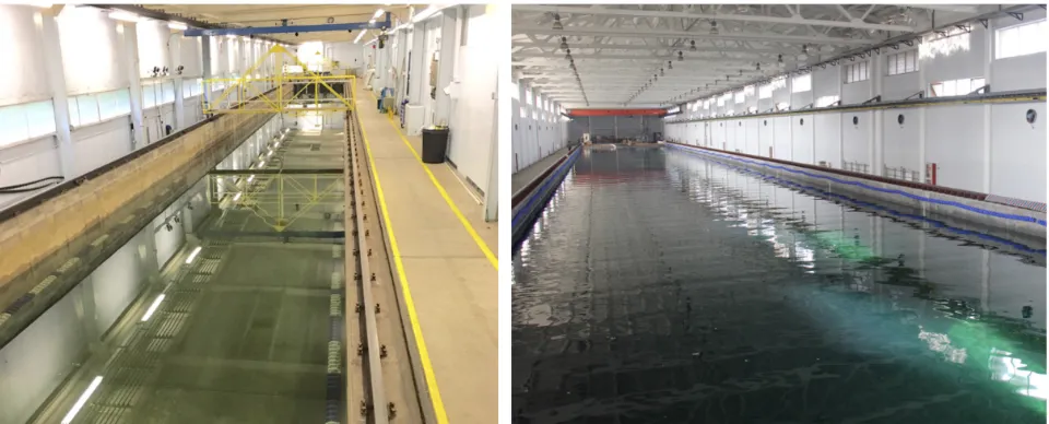
The first experiment was carried out in the multifunctional ship model towing tank at Shanghai Jiao Tong University, China. The total length of the wave tank was 300 meters and the width of the tank was 16 meters. The tank had a flat bed with a water depth of 7.5 meters, which gives a non-dimensional water depth greater thankd>3. There were 40 hinged-flap type wave makers
at one end of the flume. First-order wave generation theory was applied and the impact of second-order error wave was analysed carefully and found not to affect results. There was a parabolic beach at the far end of the flume, which was opposite to the wave makers. Reflection analysis using the least squares method [17] estimates that less than 10% of the energy is reflected. The wave surface elevation was measured by 10 capacitance probes at 100 Hz with excellent calibration characteristics. However, due to facility limitations, the wave probes could only be installed on the carriage. To track the wave evolution over a wider range, the experiment was repeated with different carriage positions. The facility is shown in Figure 1.
In the Shanghai tank only two phase decomposition was used. This was partly due to experimental time constraints but also because the spectra considered were very narrow banded. The three spectra considered were based on the classic work of Onorato et al. [18] where the object had been to investigate mod-ulation instabilities.
Kelvin tank (Strathclyde)
The second experimental campaign was undertaken at the Kelvin Hydrodynamic Laboratory in the University of Strath-clyde, Glasgow, United Kingdom. The tests were carried out in the lab’s 76 m by 4.6 m towing tank with a constant water depth of 1.8 m over a flat bottom. The tank is equipped with a ‘flap-type’ wavemaker consisting of four paddles with force-feedback at one end, and a sloping beach acting as a passive absorber at the other end. A single surface-piercing vertical cylinder of di-ameter 0.315 m was placed at the centre of the tank, 35.315 m away from the wavemaker. The location of the cylinder was po-sitioned by a laser rangefinder. The draft of the cylinder is 1.6 m. The cylinder was supported on top by a stiff frame which was attached to a load cell capable of measuring 6 degrees-of-freedom forces and moments. The load cell was fixed to the sub-carriage. The support frame of the sub-carriage is about 2.0 m
above the still water surface, to allow the possible high runup of the large focussed waves. A second load cell was installed under water at the bottom of the cylinder measuring both wave loads and overturning moment. A snapshot of the experimental setup is displayed in Figure 1.
In the Kelvin tank four phase decomposition was used. The results presented here are for a JONSWAP spectrum with γ = 3.3.
RESULTS
Focussed wave-groups
Before proceeding to analyse random timeseries we demon-strate the facilities and the basic technique using focussed wave-groups. Focussed wave-groups were generated in each of the fa-cilities using linear dispersion to approximately focus the groups at the probes (exact focussing was not important in these tests).
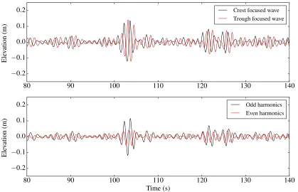
We start by looking at water surface elevation in the Shang-hai tank. A focussed NewWave (see Tromans [19]) is generated based on an underlying Pierson-Moskowitz spectrum with peak period 3.5 seconds and amplitude at focus 0.1 m and measured at 52.8 m down the tank. Figure 2 presents the timeseries of the crest and trough focussed wave-group as well as the extracted odd and even harmonics. Visually crest and trough focussed waves show good phase alignment and the extraction of odd and even harmonics appears to be clean. A second-order error wave, due to the linear generation at the paddle is observable after the signal which is, of course, in phase for both crest and trough fo-cussed events.
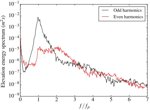
The separation of the harmonics can be more clearly seen if we examine the spectra of the measured ‘odd’ and ‘even’ har-monics. Figure 3 presents these data. The separation between odd and even harmonics can clearly be seen – indeed despite the tiny magnitude of these waves the harmonics can still be sepa-rated at f/fp=6−7.
Unlike for the free surface, where, building on the funda-mental work of Stokes, we expect a harmonic structure to the higher harmonics we do not have a similar theoretical basis, to arbitrary order, for forces on a column. Recent work [5, 11], as well as unpublished work from the De-Risk project [20], does suggest that this may be a good model for non-breaking waves on columns. Clearly for breaking waves the physics is strongly non-linear and a model based on powers of some linear time-series will not be appropriate. In this study we choose sea-states with minimal breaking. But applying this methodology to forces does require us to make more assumptions.
FIGURE 1. THE EXPERIMENTAL FACILITIES USED IN THIS STUDY. LEFT: THE KELVIN TANK; RIGHT; MULTIFUNCTIONAL SHIP MODEL TOWING TANK
80 90 100 110 120 130 140
−0.15
−0.10
−0.05
0.00
0.05
0.10
0.15
E
le
va
tio
n
(m
)
Crest focused wave Trough focused wave
80 90 100 110 120 130 140
Time (s)
−0.10
−0.05
0.00
0.05
0.10
0.15
E
le
va
tio
n
(m
)
Odd harmonics Even harmonics
FIGURE 2. WAVE GROUP PROFILES AT THE MULTIFUNC-TIONAL SHIP MODEL TOWING TANK WITH TWO PHASE DE-COMPOSITION
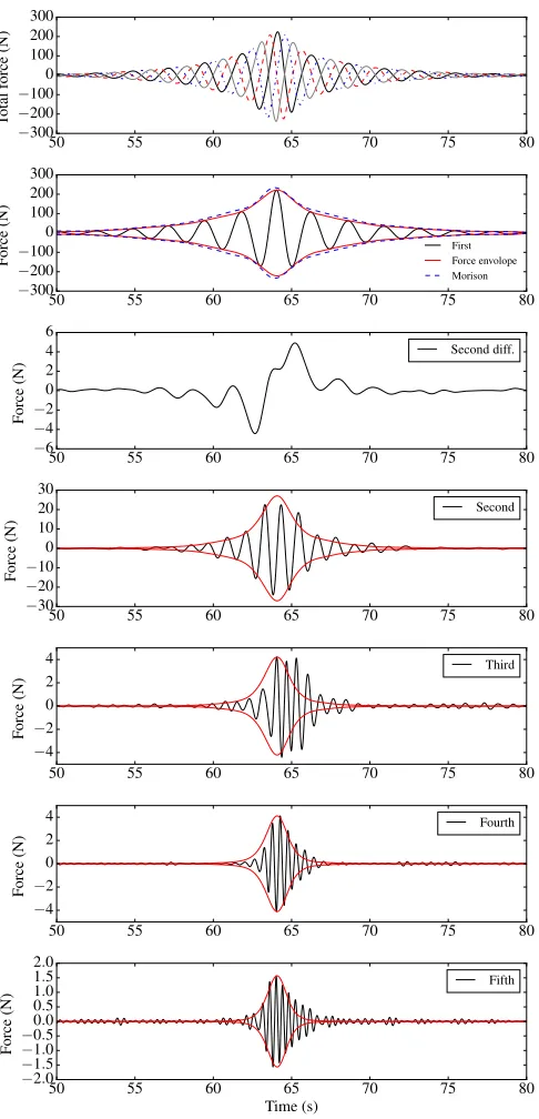
is 0.169 m. The linear force envelope in dash line is estimated by the Morison inertial formula using the linear component en-velope of the incident wave group in the absence of the cylinder. The envelopes shown in red at higher harmonics give the pre-dicted shape of each harmonic based on raising the shape of the linear signal to the relevant power. These envelopes are scaled to the maximum of the envelope of the extracted harmonic.
There is generally good agreement on the shape of the higher harmonics – they agree reasonably well with the predicted en-velopes. The worst fit is for the third harmonic, a result con-sistent with Fitzgerald et al. [5] where it is suspected additional physics is important.
0 1 2 3 4 5 6 7
f/fp
10−12
10−11
10−10
10−9
10−8
10−7
10−6
10−5
10−4
10−3
E
le
va
tio
n
en
er
gy
sp
ec
tr
um
(
m
2s)
Odd harmonics Even harmonics
FIGURE 3. WAVE SPECTRUM FOR THE WAVE GROUP AT THE MULTIFUNCTIONAL SHIP MODEL TOWING TANK WITH TWO PHASE DECOMPOSITION
Figure 5 presents the spectra of the different harmonics. Some leakage is apparent – for instance in the second order sum term there is a small spike in the linear frequency-range – how-ever this is two orders of magnitude smaller than the second order peak itself and can mostly be removed by frequency filtering. We also note that even a small amount of drag on the cylinder would also damage the Stokes like symmetry of the results.
[image:4.612.68.548.73.267.2] [image:4.612.39.288.324.484.2] [image:4.612.326.567.326.501.2]50 55 60 65 70 75 80
−300
−200
−1000
100 200 300 To ta lf or ce (N )
50 55 60 65 70 75 80
−300 −200 −100 0 100 200 300 Fo rc e (N ) First Force envolope Morison
50 55 60 65 70 75 80
−6
−4
−20
2 4 6 Fo rc e (N
) Second diff.
50 55 60 65 70 75 80
−30 −20 −10 0 10 20 30 Fo rc e (N ) Second
50 55 60 65 70 75 80
−4 −2 0 2 4 Fo rc e (N ) Third
50 55 60 65 70 75 80
−4 −2 0 2 4 Fo rc e (N ) Fourth
50 55 60 65 70 75 80
Time (s)
−2.0
−1.5
−1.0
−00..50
0.5 1.0 1.5 2.0
Fo
rc
e
(N
) Fifth
FIGURE 4. HORIZONTAL WAVE FORCES ON THE CYLIN-DER FOR THE WAVE GROUP IN THE KELVIN TANK WITH FOUR-PHASE DECOMPOSITION. TOP: INDIVIDUAL TOP SE-RIES OF FORCES FROM THE 4 EXPERIMENTS. BELOW: THE EXTRACTED TIMESERIES (WITH APPROPRIATE FREQUENCY FILTERS APPLIED) FOR DIFFERENT HARMONICS.
0 1 2 3 4 5 6 7
f/fp
10−4
10−3
10−2
10−1
100 101 102 103 104 105 Fo rc e en er gy sp ec tr um ( N
2s)
First Second sum Third
Fourth + second diff.
FIGURE 5. HORIZONTAL WAVE FORCE SPECTRUM FOR THE WAVE GROUP IN THE KELVIN TANK WITH FOUR-PHASE DE-COMPOSITION
different experimental facilities.
Random sea state
We now turn to the analysis of irregular timeseries. The wave generation is carried out in an identical way to the focus wave-groups with a linear timeseries being provided which is phase manipulated to give the desired signal.
We first consider the water surface elevations measured in the Shanghai tank. To our surprise the results were largely in-dependent of the input spectrum. Relatively close to the wave-maker the phase separation method appears to work well. Figure 6 shows sample timeseries for the most non-linear cases. It also shows the timeseries of the odd and even harmonics after the se-ries have been added and subtracted. This sea-state was based on a JONSWAP spectrum withγ=6,Hs=0.182m andTp=1.5s –
this is exceptionally steep and narrowbanded. The phase separa-tion appears to work well visually. Figure 7 shows the spectrum for this case. Due to the irregular nature of the waves the spec-tral separation is slightly less clear than for the wave-groups – however; clearly the method is essentially working.
[image:5.612.326.567.80.255.2] [image:5.612.44.287.91.595.2]80 90 100 110 120 130 140
−0.2
−0.1
0.0
0.1
0.2
E
le
va
tio
n
(m
)
Crest focused wave Trough focused wave
80 90 100 110 120 130 140
Time (s)
−0.2
−0.1
0.0
0.1
0.2
E
le
va
tio
n
(m
)
Odd harmonics Even harmonics
FIGURE 6. RANDOM WAVE PROFILES AT THE MULTIFUNC-TIONAL SHIP MODEL TOWING TANK WITH TWO PHASE DE-COMPOSITION METHOD AT 11.36 M FROM THE WAVEMAKER
0 1 2 3 4 5 6 7
f/fp
10−9
10−8
10−7
10−6
10−5
10−4
10−3
10−2
10−1
E
le
va
tio
n
en
er
gy
sp
ec
tr
um
(
m
2s)
Odd harmonics Even harmonics
FIGURE 7. WAVE SPECTRUM FOR THE RANDOM WAVES AT THE MULTIFUNCTIONAL SHIP MODEL TOWING TANK WITH TWO PHASE DECOMPOSITION METHOD AT 11.36 M FROM THE WAVEMAKER
clearly some cancellation working – the even harmonics are sig-nificantly below the odd harmonics in the linear frequency range. However, the extraction of the different harmonics is clearly not clean enough to be useful without further manipulation.
We do not fully understand why the method works well close to the paddle but then fails further down the tank. The obvious suggestion is that this is due to wave-breaking the exact loca-tion at which this happens being strongly linked to the phase of the wave. Close to the paddle very little breaking was observed for all cases (presumably due to breaking at the paddle of very
large waves). However, for the least non-linear case, very little breaking was observed at any point in the tank. Hence, wave breaking does not appear to be a fully satisfactory hypothesis to explain all the results. An alternative explanation might be due to modulation instabilities leading to the phase alignment failing. The tests do show good agreement with the evolution of kurtosis down the tank (see Janssen [21] and Figure 1 in [22]) although these results are not presented here. However, this should not ob-viously lead to the changes in phase which lead to the breakdown of the method observed experimentally. Third order interactions should not be a problem for this approach however 4th order (5-wave interaction) would break the symmetry pattern as crests and troughs would then start to behave differently.
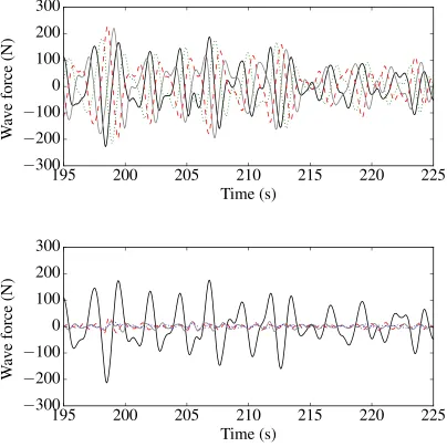
We next turn to the analysis of forces. Unlike the free surface data from the Shanghai tank, we effectively only sample these at one point along the tank. Figure 10 presents a sample timeseries of the total inline force measured on the column. The four differ-ent timeseries can be seen approximately 90◦out of alignment.
These can be combined together to extract timeseries for the dif-ferent harmonics also shown in the figure. Figure 11 presents the spectrum of the force timeseries. There appears to be a very clean separation of the linear force around the spectral peak. Of the other harmonics the ‘third’ appears the most questionable, whilst as expected this is the largest component around 3 to 4 fp
this signal is surprisingly large (relative to the other harmonics) for lower frequencies. The reason for this is unclear. The extrac-tion is clearly less clean than for the isolated wave-groups. This may be due to reflections into the tank or, as discussed above, to breaking waves.
CONCLUSIONS
In this paper we have considered whether phase manipula-tion can be used to extract ‘slave’ harmonics from random time-series extending its existing application to wave-groups. We con-sidered both wave elevation measurements as well as forces on a surface piercing column. Our findings are somewhat mixed. The basic technique clearly works in theory, and the fact that we can get acceptable results out implies that contamination from reflec-tions and similar issues which are inevitable in random wave tests are typically not sufficient to invalidate the approach. However, the method clearly broke down for some tests where we would have expected it to work. An advantage of the method is that it is reasonably clear where it breaks down. Further work needs to be carried out to understand why the method failed.
[image:6.612.39.288.78.239.2] [image:6.612.44.285.313.490.2]80 90 100 110 120 130 140
−0.2
−0.1
0.0
0.1 0.2
E
le
va
tio
n
(m
)
Crest focused wave Trough focused wave
80 90 100 110 120 130 140
Time (s)
−0.2
−0.1 0.0
0.1
0.2
E
le
va
tio
n
(m
)
Odd harmonics Even harmonics
FIGURE 8. RANDOM WAVE PROFILES AT MULTIFUNCTIONAL SHIP MODEL TOWING TANK WITH TWO PHASE DECOMPOSITION METHOD AT 68 M FROM THE PADDLE
approach described in the present paper gives us full timeseries of the bound harmonics. Nevertheless, it would be interesting to compare the two approaches in detail.
REFERENCES
[1] Walker, D. A. G., Taylor, P. H., and Eatock Taylor, R., 2004. “The shape of large surface waves on the open sea and the draupner new year wave”.Applied Ocean Research, 26
(3-4), pp. 73–83.
[2] Adcock, T. A. A., and Taylor, P. H., 2009. “Estimating ocean wave directional spreading from an eulerian surface elevation time history”. Proceedings of the Royal Society of London A: Mathematical, Physical and Engineering Sci-ences, 465(2111), pp. 3361–3381.
[3] Gibbs, R. G., 2004. Walls of Water on the Open Ocean. DPhil Thesis, University of Oxford, Trinty term.
[4] Jonathan, P., and Taylor, P. H., 1997. “On irregular, nonlin-ear waves in a spread sea”. Journal of Offshore Mechanics and Arctic Engineering, 119(1), pp. 37–41.
[5] Fitzgerald, C. J., Taylor, P. H., Eatock Taylor, R., Grice, J., and Zang, J., 2014. “Phase manipulation and the har-monic components of ringing forces on a surface-piercing
column”.Proc. R. Soc. A, 470(2168), p. 20130847.
[6] Hann, M., Greaves, D., and Raby, A., 2014. “A new set of focused wave linear combinations to extract non-linear wave harmonics”. In Twenty-ninth Int. Workshop on Water Waves and Floating Bodies, pp. 61–64.
[7] Hunt, A., Taylor, P., Borthwick, A., Stansby, P., and Feng, T., 2004. “Kinematics of a focused wave group on a plane beach: Physical modeling in the uk coastal research facil-ity”. InCoastal Structures 2003. pp. 740–750.
[8] Gibbs, R. G., and Taylor, P. H., 2005. “Formation of wall of water in ‘fully’ nonlinear simulations”. Applied Ocean Research, 27(3), pp. 142–157.
[9] Hunt-Raby, A. C., Borthwick, A. G. L., Stansby, P. K., and Taylor, P. H., 2011. “Experimental measurement of focused wave group and solitary wave overtopping”.Journal of Hy-draulic Research, 49(4), pp. 450–464.
[10] Adcock, T. A. A., Gibbs, R. H., and Taylor, P. H., 2012. “The nonlinear evolution and approximate scaling of direc-tionally spread wave groups on deep water”. Proc. R. Soc. A, 468(2145), pp. 2704–2721.
[image:7.612.97.516.81.351.2]0 1 2 3 4 5 6 7 f/fp
10−9
10−8
10−7
10−6
10−5
10−4
10−3
10−2
10−1
E
le
va
tio
n
en
er
gy
sp
ec
tr
um
(
m
2s)
Odd harmonics Even harmonics
FIGURE 9. WAVE SPECTRUM FOR RANDOM WAVES AT MUL-TIFUNCTIONAL SHIP MODEL TOWING TANK WITH TWO PHASE DECOMPOSITION METHOD 68 M FROM THE PADDLE
surface-piercing column: Stokes-type expansions of the force harmonics”. Journal of Fluid Mechanics, 848,
pp. 42–77.
[12] McAllister, M. L., Adcock, T. A. A., Taylor, P. H., and van den Bremer, T. S., 2018. “The set-down and set-up of directionally spread and crossing surface gravity wave groups”.Journal of Fluid Mechanics, 835, pp. 131–169.
[13] Vyzikas, T., Stagonas, D., Buldakov, E., and Greaves, D., 2018. “The evolution of free and bound waves during dispersive focusing in a numerical and physical flume”.
Coastal Engineering, 132, pp. 95–109.
[14] Zhao, W., Wolgamot, H. A., Taylor, P. H., and Eatock Tay-lor, R., 2017. “Gap resonance and higher harmonics driven by focused transient wave groups”. Journal of Fluid Me-chanics, 812, pp. 905–939.
[15] Whittaker, C. N., Raby, A. C., Fitzgerald, C. J., and Tay-lor, P. H., 2016. “The average shape of large waves in the coastal zone”.Coastal Engineering, 114, pp. 253–264.
[16] Longuet-Higgins, M. S., 1987. “The propagation of short surface waves on longer gravity waves”. Journal of Fluid Mechanics, 177, pp. 293–306.
[17] Mansard, E. P. D., and Funke, E. R., 1980. The Mea-surement of Incident and Reflected Spectra Using a Least Squares Method.
[18] Onorato, M., Osborne, A. R., Serio, M., and Bertone, S., 2001. “Freak Waves in Random Oceanic Sea States”.Phys. Rev. Lett., 86(25), jun, pp. 5831–5834.
[19] Tromans, P. S., Anaturk, A. R., Hagemeijer, P., et al., 1991. “A new model for the kinematics of large ocean waves-application as a design wave”. In The First International
Offshore and Polar Engineering Conference, International Society of Offshore and Polar Engineers.
[20] Bredmose, H., Dixen, M., Ghadirian, A., Larsen, T. J., Schløer, S., Andersen, S. J., Wang, S., Bingham, H. B., Lindberg, O., Christensen, E. D., Engsig-Karup, A. P., Pe-tersen, O. S., Hansen, H. F., Mariegaard, J. S., Taylor, P. H., Adcock, T. A. A., Obhrai, C., Gudmenstad, O. T., Tarp-Johansen, N. J., Meyer, C. P., Krokstad, J. R., Suja-Thauvin, L., and Hanson, T. D., 2016. “DeRisk–Accurate prediction of ULS wave loads. Outlook and first results”.
Energy Procedia, 94, pp. 379–387.
[21] Janssen, P. A. E. M., 2003. “Nonlinear four-wave interac-tions and freak waves”.Journal of Physical Oceanography,
33(4), pp. 863–884.
[image:8.612.45.285.80.257.2]