A numerical study of strain localization in elasto-thermo-viscoplastic materials using radial basis function networks

A Numerical Study of Strain Localization in Elasto-Thermo-Viscoplastic

Materials using Radial Basis Function Networks

P. Le1 N. Mai-Duy1 T. Tran-Cong1 and G. Baker2

Abstract: This paper presents a numerical sim-ulation of the formation and evolution of strain lo-calization in elasto-thermo-viscoplastic materials (adiabatic shear band) by the indirect/integral ra-dial basis function network (IRBFN) method. The effects of strain and strain rate hardening, plas-tic heating, and thermal softening are considered. The IRBFN method is enhanced by a new coor-dinate mapping which helps capture the stiff spa-tial structure of the resultant band. The discrete IRBFN system is integrated in time by the implicit fifth-order Runge-Kutta method. The obtained results are compared with those of the Modified Smooth Particle Hydrodynamics (MSPH) method and Chebychev Pseudo-spectral (CPS) method.

Keyword: Shear band, strain localization, RBFN, imperfection, shear band formation.

1 Introduction

Strain localization in elasto-thermo-visco-plastic materials is a phenomenon that occurs during high strain-rate plastic deformation, such as machin-ing, forgmachin-ing, shock impact loadmachin-ing, ballistic im-pact and penetration, and has been proposed as an explanation for deep earthquakes [Walter (1992)]. In particular, a shear band is a narrow, nearly planar or two dimensional region of very large shear strain and strain rate. The formation of shear bands often precedes the rupture in mate-rials. Even when the rupture does not occur, the development of shear bands generally reduces the performance of the material. Hence, an under-standing of shear-band morphology and evolution is an important prerequisite to improve material

1_{CESRC, University of Southern Queensland,}

Toowoomba, QLD 4350, Australia.

2_{DVC(S), University of Southern Queensland,}

Toowoomba, QLD 4350, Australia.

Belytschko, Kulkarni, and Lott-Crumpler (1994)] is particularly effective and efficient, but gener-ally restricted to simple geometries. The finite el-ement method (FEM) [Wright and Walter (1987); Batra and Kim (1991); Walter (1992)] has been used to analyze shear strain localization prob-lems with good results for 1D cases, since the Lagrangian finite element mesh is not badly dis-torted and small element size ofO(10−7)enables one to capture the high strain. However, the FEM has many drawbacks in 2D or 3D strain local-ization problems. In contrast to the FEM, mesh-less methods [ Atluri and Zhu (1998); Li and Liu (2000); Batra and Zhang (2004); Atluri and Shen (2002); Han and Atluri (2003); Han and Atluri (2004); Han, Rajendran, and Atluri (2005); Han, Liu, Rajendran, and Atluri (2006)] offer some ad-vantages, including (i) shape functions are con-structed by using a highly smooth window func-tion, (ii) purely displacement-based formulation is possible without incurring volumetric locking within a range of support size of the window functions [Li and Liu (2000)], and (iii) approx-imations are non-local. Thus, meshless meth-ods provide more continuous solutions than the piece-wise continuous ones obtained by the FEM. These properties provide an effective remedy for the mesh alignment sensitivity in the computation of strain localization.

In this study, we report a new numerical method based on radial basis function networks, a truly meshless method, for analysis of the dynamics of strain localization in 1D problems. The present indirect/integral radial basis function network (IRBFN) method is based on (i) the universal ap-proximation property of RBF networks, (ii) expo-nential convergence characteristics of the chosen multiquadric (MQ) RBF, (iii) a simple point col-location method of discretisation of the governing equations, and (iv) an indirect/integral (IRBFN) rather than a direct/differential (DRBFN) ap-proach [Kansa (1990)] for the approximation of functions and derivatives. For the DRBFN, Madych and Nelson (1990) showed that the con-vergence rate is a decreasing function of deriva-tive order. Since the introduction of the IRBFN approach by [Mai-Duy and Tran-Cong (2001);

Mai-Duy and Tran-Cong (2005)], Kansa, Power, Fasshauer, and Ling (2004), and Ling and Trum-mer (2004), based on the theoretical result of Madych and Nelson (1990), concluded that the decreasing rate of convergence can be avoided in the IRBFN approach. Furthermore, the inte-gration constants arisen in the IRBFN approach are helpful in dealing with problems with mul-tiple boundary conditions [Mai-Duy and Tran-Cong (2006)]. In addition, a new coordinate map-ping is here introduced to help capture the char-acteristics of extremely thin boundary layers (i.e. the localised shear bands). The paper is organized as follows. The physical problem and its mathe-matical model are defined in section 2. The nu-merical formulation of the mathematical model is presented in section 3 which is followed by nu-merical examples in section 4. Some conclusions are drawn in section 5.

2 Problem definition

We consider the unidirectional shearing of an in-finite slab of half thicknessH, and of an elasto-thermo-viscoplastic material. In this section we use the overbar to represent dimensional quan-tities, the subscript comma to denote the partial differentiation with respect to the variable indi-cated by the subscript. The unknowns are the shear stresss, the particle velocityv, the plastic strainγ and the temperature measured from the reference valueΘ. In addition, the strain harden-ing parameter Ψis also introduced as in [Walter (1992); Bayliss, Belytschko, Kulkarni, and Lott-Crumpler (1994)].

Lety be the coordinate across the slab with ori-gin on the middle plane, i.e. −H ≤y≤H, and

t denote time. The mathematical model for this problem can be found in [Walter (1992); Wright (2002); Bayliss, Belytschko, Kulkarni, and Lott-Crumpler (1994)] and is reproduced here as fol-lows.

v_,t = s_,y

ρ, (1a)

ρcΘ_,t=kΘ_,yy+sγ_,t, (1c)

Ψ_,t= sγ_,t

κ(Ψ), (1d)

whereρ is the density,cthe specific heat, k the thermal conductivity,μ the shear modulus, andκ a strain hardening factor. The constitutive relation betweens,Ψ,Θandγ_,t is given by

s=κ(Ψ)g(Θ)f(γ_,t), (2)

wherega thermal softening factor, and f a strain rate hardening factor. Different material models can be obtained with appropriate choices of these factors, which will be illustrated when we con-sider examples in section 4. The problem is as-sumed to be symmetric about the middle plane

y=0. The slab is subjected to a constant shearing velocity±v0prescribed at the top and bottom sur-faces of the slab, respectively. The sursur-faces are thermally insulated and all plastic work is con-verted into heat. The above assumptions lead to the following boundary conditions

v(0,t) =0, v(H,t) =v0, Θ,y(0,t) =0, Θ,y(H,t) =0.

(3)

The nominal strain rate is

˙ γ0

=γ0 ,t=

v0

H, (4)

where the time derivatives are from now on indi-cated by a dot over the variable. The variables are non-dimensionalised as follows.

y=_Hy, t=tγ˙0, Ψ˙ = Ψ_˙˙ γ0, v=

v

Hγ˙0, s= s

κ0,

Θ=ρcΘ

κ0 , κ=_κκ0, γ˙=

˙ γ ˙

γ0, k= k

ρcH2γ˙0,

ρ=ρH2(γ˙0)2

κ0 , μ=

μ

κ0, b=bγ˙

0

, a=a_ρκ_c0,

where ais the thermal softening parameter, b is the strain-rate hardening parameter,κ0is the yield stress in the quasi-static isothermal simple shear test. The dimensionless governing equations are given by

˙

v=s,y

ρ, (5a)

˙

s=μ(v_,y−γ˙), (5b)

˙

Θ=kΘ_,yy+sγ˙, (5c)

˙

Ψ= sγ˙

κ(Ψ). (5d)

The constitutive relation is

s=κ(Ψ)g(Θ)f(γ˙). (6)

The boundary conditions are

v(0,t) =0, v(1,t) =1,

Θ,y(0,t) =0, Θ,y(1,t) =0. (7)

From Eq. 5a and Eq. 7, the boundary conditions for shear stress can be found easily as

s_,y(0,t) =0, s_,y(1,t) =0. (8)

We will present a meshless numerical method for solving Eq. 5a-Eq. 8 in the next section, and in section 4 we will present results for two particular models, namely the thermal imperfection and the strength imperfection cases.

3 Numerical formulation

Consider an initial-boundary-value problem gov-erned by the second order PDE

∂u

∂t =a

∂2_u ∂x2 +b

∂u

∂x+cu+d, (9)

wherea,b,canddare the coefficients, 0≤t≤T

andxmin≤x≤xmax, with the boundary and initial

conditions

u(t,xmin) =u1, (10)

∂u

∂x|(t,x=xmax)=u

N, (11)

u(0,x) =g(x), (12)

in whichu1anduNare given values, andg(x)is a

3.1 Spatial discretisation

In the indirect RBF method (see [Mai-Duy and Tran-Cong (2001); Mai-Duy and Tran-Cong (2005); Mai-Duy (2005); Mai-Duy and Tan-ner (2005)]), the formulation of the problem starts with the decomposition of the highest or-der or-derivative unor-der consior-deration into RBFs. The derivative expression obtained is then integrated to yield expressions for lower order derivatives and finally for the original function itself. The present work is concerned with the approximation of a function and its derivatives of order up to 2, the formulation can be thus described as follows [Mai-Cao and Tran-Cong (2005)]

d2u(x,t) dx2 =

m

∑

wi(t)gi(x) = m

∑

wi(t)H_i[2](x),

(13)

du(x,t)

dx =

m

∑

wi(t)gi(x)dx+c1(t)

=

∑

wi(t)

gi(x)dx+c1(t)

=

∑

wi(t)H_i[1](x) +c1(t), (14)

u(x,t) = m

∑

wi(t)

H_i[1](x)dx+c1(t)x+c2(t)

=

∑

wi(t)H_i[0](x) +c1(t)x+c2(t),

(15)

wheremis the number of RBFs,{gi(x)}m i=1is the set of RBFs, {wi(t)}m_i=1 is the set of correspond-ing network weights to be found and{H_i[.](x)}m_i=1

are new basis functions obtained from integrating the radial basis functiongi(x). The multiquadrics function is chosen in the present study

gi(x) =

(x−ci)2_+a2

i, (16)

where ci is the RBF centre and ai is the RBF

width. The width of the ith RBF can be deter-mined according to the following simple relation

ai=βdi, (17)

whereβ is a factor,β >0, anddi is the distance

from theith centre to its nearest centre. To have

the same coefficient vector as Eq. 15, expressions Eq. 13 and Eq. 14 can be rewritten as follows

d2u(x,t) dx2 =

m

∑

wi(t)H_i[2](x) +c1(t).0+c2(t).0,

(18)

du(x,t)

dx =

m

∑

wi(t)H_i[1](x) +c1(t).1+c2(t).0.

(19)

Here we choose the RBF centrescito be identical to the collocation pointsxi, i.e.{ci}m_i=1={xi}N_i=1. The evaluation of Eq. 18, Eq. 19 and Eq. 15 at a set ofNcollocation points leads to

u(t) = H[2]w(t), (20) u(t) = H[1]w(t), (21) u(t) = H[0]w(t), (22)

where

u(t) =

∂2_u 1(t) ∂x2 ,

∂2_u 2(t)

∂x2 ,...,

∂2_uN(t) ∂x2

T

, (23)

u(t) =

∂u1(t) ∂x ,

∂u2(t)

∂x ,...,

∂uN(t)

∂x

T

, (24)

u(t) = [u1(t),u2(t),...,uN(t)]T, (25)

H[2]=

⎛ ⎜ ⎜ ⎜ ⎜ ⎝

H₁[2](x1) H₂[2](x1) ··· H_N[2](x1) 0 0

H₁[2](x2) H₂[2](x2) ··· HN[2](x2) 0 0 ..

. ... . . . ... ... ...

H₁[2](xN) H₂[2](xN) ··· H_N[2](xN) 0 0 ⎞ ⎟ ⎟ ⎟ ⎟ ⎠, (26)

H[1]=

⎛ ⎜ ⎜ ⎜ ⎜ ⎝

H₁[1](x1) H₂[1](x1) ··· HN[1](x1) 1 0

H₁[1](x2) H2[1](x2) ··· HN[1](x2) 1 0 ..

. ... . . . ... ... ...

H[0]= ⎛ ⎜ ⎜ ⎜ ⎜ ⎝

H₁[0](x1) H₂[0](x1) ··· HN[0](x1) x1 1

H₁[0](x2) H₂[0](x2) ··· HN[0](x2) x2 1 ..

. ... . . . ... ... ...

H₁[0](xN) H₂[0](xN) ··· H_N[0](xN) xN 1 ⎞ ⎟ ⎟ ⎟ ⎟ ⎠, (28) and

w(t) = [w1(t),...,wN(t),c1(t),c2(t)]T. (29) From an engineering point of view, it would be more convenient to work in the physical space. Owing to the presence of integration constants, the process of converting the networks-weight space into the physical space can also be used to implement Neumann boundary conditions. With the boundary conditions Eq. 10 and Eq. 11, the conversion system can be employed as

u(t) u_N(t)

=Cw(t), (30)

where C is the conversion matrix of dimension

(N+1)×(N+2)that comprises the matrixH[0] and the last row ofH[1]. Solving Eq. 30 yields

w(t) =C−1

u(t) u_N(t)

. (31)

By substituting Eq. 31 into Eq. 20 and Eq. 21, the values of the second and first derivatives ofuwith respect tox are thus expressed in terms of nodal variable values and Neumann boundary value

u(t) =H[2]C−1

u(t) u_N(t)

=D[2]

u(t) uN(t)

, (32)

u(t) =H[1]C−1

u(t) uN(t)

=D[1]

u(t) uN(t)

. (33)

Making use of Eq. 32 and Eq. 33, equation Eq. 9 can be transformed into the following discrete form

du(t) dt =au

_{(t) +bu(t) +cu(t) +d, (34)}

or

du

dt =

aD[2]

u(t) u_N(t)

+bD[1]

u(t) u_N(t)

+cu(t) +d,

(35)

whered= [d,d,...d]T is anN×1 vector, and

du

dt =

du1(t)

dt , du2(t)

dt ,...,

duN(t) dt

T

. (36)

Since the values ofu1 anduN are given, the

un-known vector becomes

[u2(t),u3(t),...,uN(t)]T, (37)

and hence, the first row in Eq. 35 will be removed from the solution procedure. The remainder of Eq. 35 can be integrated in time by using standard solvers such as the Runge-Kutta technique.

3.2 Resolution of very large spatial gradients

It has been shown that the IRBFN method can capture sharp gradients in some PDE solutions [Mai-Duy and Tran-Cong (2003)] with relatively coarse uniform spatial discretisation. However, with extremely sharp gradients in a solution, the option of uniformly refining the discretisation is not efficient or even effective. The computing of such extremely sharp gradients can be achieved effectively and efficiently with appropriate coor-dinate mappings of a relatively coarse, originally uniform discretisation. A very good mapping can be introduced as follows.

Consider the singularly perturbed boundary value problem (BVP)

εu(x) +p(x)u(x) +q(x)u(x) = f(x),

∀x∈[a,b], (38)

subject to the boundary conditions

u(a) =ua, u(b) =ub, (39)

layer of widthO(ε), then on a uniform grid with

O(N−1_{) spacing between the points we would} needN=O(ε−1), which is not practical in most cases.

We transform the BVP Eq. 38 via the variable transformationx −→y(x)into a new BVP

εv(y)y(x)2+P(y)v(y) +Q(y)v(y) =F(y), ∀y∈[a,b], (40)

subject to boundary conditions

v(a) =ua, v(b) =ub, (41)

wherev(y) =u(x(y)), and the transformed coeffi-cients are given by

P(y) =εy(x) +p(x)y(x), Q(y) =q(x),

F(y) = f(x). (42)

In this mapping,x represents the physical space andythe computational space.

Without loss of generality, we assume that[a,b] =

[−1,1]. Consider the one-to-one mapping given by

x(y) =sinh(αy)

sinh(α) , (43)

where α >0 is a parameter that allows control of the discretisation, the smaller the value ofε is, the larger the value ofα is required. From Eq. 43 the inverse mapping and the derivatives ofywith respect toxcan be determined simply

y(x) =arcsinh(λx)

α , (44)

y(x) = λ (1+λ2_x2₎12α

, (45)

y(x) = −λ

3_x

(1+λ2_x2)32α

, (46)

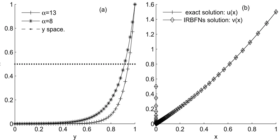
where λ = sinh(α). As shown in the Figure 1(a), the physical space x is very dense around the layer’s locationx=0 while the computational spaceyis uniform.

Note that the transform Eq. 43 also maps the in-terval[−1,0]and[0,1]onto themselves. Hence,

if Eq. 38 has only one boundary layer on the left (or central or right), we can translate the physical space to[−1,0](or[−1,1]or[0,1]) to avoid un-necessary collocation points in the non-steep re-gion.

To illustrate the above mapping, we let p(x) =1,

q(x) =0, f(x) =x+1+ε,[a,b] = [0,1],ua=0.5

andub=1.5 in Eq. 38, obtaining

εu(x) +u(x) =x+1+ε, ∀x∈[0,1],

u(0) =0.5, u(1) =1.5, (47)

which has an exact solution given by

u(x) = 1

2

e−εx+x2+2x

. (48)

For ε =10−6, the IRBFN solution in the physi-cal space with 61 collocation points,α =13, are shown in the Figure 1(b), which shows that the numerical solution is quite indistinguishable from the exact solutions. Forε =10−12, we can cap-ture an accurate solution by using 161 collocation points andα=29.

4 Numerical examples

4.1 Example 1: A model of thermal

imperfec-tion

In this example we consider a specific case of the general unidirectional shearing problem defined in section 2 where the thermal softening factor in Eq. 6 is given by

g(Θ) = (1−aΘ), (49)

the strain hardening factor by

κ(Ψ) =

1+ Ψ Ψ0

n

, (50)

and the strain rate hardening factor by

f(γ˙) = (1+bγ˙)m. (51)

0 0.2 0.4 0.6 0.8 1 0

0.2 0.4 0.6 0.8 1

y

x

α=13

α=8 y space.

0 0.2 0.4 0.6 0.8 1

0 0.2 0.4 0.6 0.8 1 1.2 1.4 1.6

x exact solution: u(x) IRBFNs solution: v(x)

(a) (b)

Figure 1: (a) Coordinate mapping with 61 collocation points, uniformly spaced in the computational space

y, (b) IRBFN solutionv(x)and exact solutionu(x)of Eq. 47 withε=10−6,α=13,on the physical space

x.

v(0,y) =y, Ψ(0,y) =0.1 , γ=0.0692, Θ(0,y) =0.1003+0.1(1−y2₎9_e−5y2

,

s(0,y) =1+0_Ψ.10

n

(1−aΘ(0,y))(1+b)m, where the second term on the right-hand side of the expression for the temperature Θ represents a thermal imperfection. With the half thickness of the slab H=2.58mm, the nominal strain rate isγ0_t =500s−1and the dimensionless parameters are

ρ=3.982×10−5, μ=240.3 , a=0.4973 ,

n=0.09 , κ=3.978×10−3_{, Ψ0=0.017 ,}

m=0.025 , b=5×10−6.

The discretisation of the governing equations yields a system of fully coupled, stiff and nonlin-ear ordinary differential equations (ODEs) which are integrated with respect to timet using an im-plicit 5th Runge-Kutta method with subroutine RADAU5 developed by Hairer, Norsett, and Wan-ner (1987), and Hairer and WanWan-ner (1996). The subroutine automatically adjusts the time step size to compute the solutions within the prescribed ac-curacy. The results presented in this paper are ob-tained by settingRT OL=10−7andAT OL=10−7 in RADAU5.

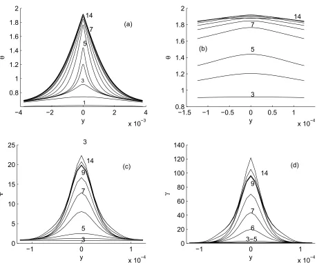
The results presented in this section are obtained with 261 collocation points and the value of α in the mapping Eq. 43 is 9, β in Eq. 17 is 1. The evolutions of the spatial profile of the tem-peratureΘ, plastic strainγ, and strain hardening parameter Ψ, are shown in Figure 2; the plas-tic strain rate in Figure 3; stress and velocity in Figure 4. These figures show that the solution is highly consistent with the boundary conditions aty=0 (and aty=±1, although not shown on the plots). From Figure 2 it can be observed that the plastic strain increases rapidly in the neigh-bourhood ofy=0 where the band of high shear strains becomes less and less diffuse, reaching a minimum with a very high corresponding plastic strain level before becoming more and more dif-fuse again. Similar patterns of development are observed for the temperature, strain hardening pa-rameter, plastic strain rate and velocity as shown in Figures 3 and 4. In contrast, the spatial profile of stress evolves slightly differently which will be discussed in more detail later.

í4 í2 0 2 4

x 10í3 0.8

1 1.2 1.4 1.6 1.8 2

y

θ

1

3 5

7 14

í1.5 í1 í0.5 0 0.5 1

x 10í4 0.8

1 1.2 1.4 1.6 1.8 2

y

θ

3 5 7

14

í1 0 1

x 10í4 0

5 10 15 20 25

y

Ψ

3 5 7 9

14

í1 0 1

x 10í4 0

20 40 60 80 100 120 140

y

γ

3í5 6 7 9

14 3

(a)

(b)

(c) (d)

Figure 2: The curve labels indicate time levels (μs): 1(59.489); 2(60.257); 3(60.433); 4(60.477); 5(60.507); 6(60.602); 7(60.702); 8(60.804); 9(60.903); 10(60.934); 11(60.975); 12(60.992); 13(61.003); 14(61.019). (a) Evolution of temperature, (b) the temperature in the neighbourhood ofy=0 showing that the solution is highly consistent with the boundary conditions aty=0, (c) evolution ofΨ, (d) evolution of plastic train.

define the limit of the high shear band as the position where the temperature equals 40% of the peak temperature at the centre of the band (This criterion is somewhat arbitrary, for exam-ple, Batra and Zhang (2004) used a value of 40% while Bayliss, Belytschko, Kulkarni, and Lott-Crumpler (1994) preferred 50%). The band-width evolves with time, for example when the plastic strain rate at y = 0 reaches its maxi-mum value (at t = 60.8385μs), the extent of the corresponding bandwidth is y=±0.00252. Hence the width of the shear band is 2× 0.00252×2580 = 13.0μm. The dimension-less half bandwidths correspond to different time

levels (in parentheses) are 0.0688 (3),0.0257 (4),0.0102 (5),0.00279 (6),0.00237 (7),0.002468 (8),0.00264 (9),0.00274 (10),0.00276 (11), which indicate that the shear band becomes narrowest (around time level 7 or 60.702μs) before the plastic strain rate peaks between time levels 8 (60.804μs) and 9 (60.903μs).

í0.040 í0.02 0 0.02 0.04 20

40 60 80 100 120

y

plastic strain rate

1

í0.0150 í0.01í0.005 0 0.005 0.01

100 200 300 400 500 600 700

y

plastic strain rate

2

í1.5 í1 í0.5 0 0.5 1 1.5

x 10í3 0

1000 2000 3000 4000 5000 6000 7000

y

plastic strain rate 3

í1 0 1

x 10í4 0

5 10

15x 10

5

y

plastic strain rate

4 5 6 9 8 7

10 11

(a) (b)

(c)

(d)

13

12

14

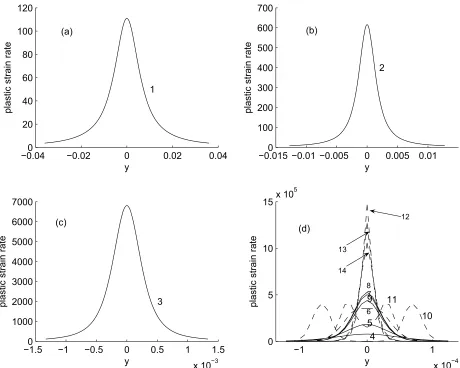
Figure 3: The evolution of plastic strain rate ˙γ. The curve labels indicate time levels (μs): 1(59.489); 2(60.257); 3(60.433); 4(60.477); 5(60.507); 6(60.602); 7(60.702); 8(60.804); 9(60.903); 10(60.934); 11(60.975); 12(60.992); 13(61.003); 14(61.019).

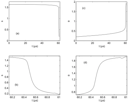
time progresses, the increase in plastic work causes increase in Θ and the thermal softening effect tends to compensate the strain and strain rate hardening effects. In the next phase of the evolution,Θ increases very slowly (Figure 5(c)) and the thermal softening effect becomes gradu-ally stronger than strain and strain rate hardening effects, and the shear stress decreases very slowly as shown in Figure 5(a). Further evolutions of the stress and velocity profiles indicate unstable de-velopment, i.e. the shear stress aty=0 is decreas-ing rapidly and the two halves of the slab (corre-sponding toH≥y>0 and−H≤y<0) are shear-ing relative to each other increasshear-ingly like rigid bodies. The instability can be seen more clearly

evo-í1 í0.5 0 0.5 1 0

0.5 1 1.5

y

s

1 3

5

7 9 14

í1 í0.5 0 0.5 1

í15

í10

í5

0 5 10 15

y

v 3

5 7 9 14

í2 0 2 4

x 10í4

í15

í10

í5

0 5 10 15

y

v 3

4 5 6 7 89,10,11

10 11 12,13, 14

í1 0 1 2

x 10í4 0

0.5 1 1.5

y

s

1 3

5

7

9í10...14 (a)

(b)

(c)

(d)

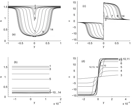
Figure 4: The curve labels indicate time levels (μs): 1(59.489); 2(60.257); 3(60.433); 4(60.477); 5(60.507); 6(60.602); 7(60.702); 8(60.804); 9(60.903); 10(60.934); 11(60.975); 12(60.992); 13(61.003); 14(61.019). (a) Spatial structure of shear stress at different times, (b) the shear stress in the neighbourhood of y=0 showing that the solution is highly consistent with the boundary conditions aty=0, (c) spatial structure of particles velocity at different times of localization, (d) the structure of the velocity boundary layer.

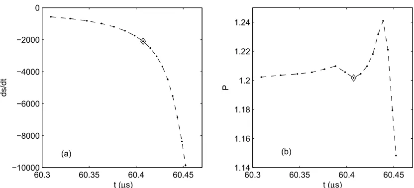
lution is smooth and therefore it is not possible to define the onset of instability uniquely. Here we define the onset of the strain localization in-stability as the point when the rate of change of stress with time continues to increase monotoni-cally and rapidly. We detect this point by examin-ing the ratioPdefined as

P= ds dt|tn+1

ds dt|tn

, (52)

for several time levels n. The instability is thus found to occur att=60.407μs as shown in Fig-ure 7. FigFig-ures 2, 3, 4 show that the interaction

soft-0 20 40 60 0

0.5 1 1.5

t (μs)

s

60.2 60.4 60.6 60.8 61 0.2

0.4 0.6 0.8 1 1.2 1.4

t (μs)

s

0 20 40 60 0

0.5 1 1.5 2

t (μs)

θ

60.2 60.4 60.6 60.8 61 0.8

1 1.2 1.4 1.6 1.8

t (μs)

θ

(a)

(b)

(c)

(d)

Figure 5: (a) and (b) evolution of shear stress aty= 0, (c) and (d) evolution of temperature aty= 0.

60.4 60.6 60.8 61 0

5 10 15x 10

5

t (μs)

plastic strain rate

60.4 60.6 60.8 61 0

20 40 60 80 100 120 140

t (μs)

plastic strain (

γ

)

(a) (b)

60.3 60.35 60.4 60.45

í10000

í8000

í6000

í4000

í2000

0

t (μs)

ds/dt

60.3 60.35 60.4 60.45

1.14 1.16 1.18 1.2 1.22 1.24

t (μs)

P

(a) (b)

Figure 7: The behaviour of the shear stress aty=0 around the onset of localisation.Pis defined by Eq. 52.

60.9 60.95 61

0.18 0.19 0.2 0.21 0.22 0.23

t (μs)

s

60.9 60.95 61

0 5 10 15x 10

5

t (μs)

plastic strain rate

60.9 60.95 61

1.88 1.89 1.9 1.91 1.92

t (μs)

θ

60.9 60.95 61

95 100 105 110 115 120 125

t (μs)

plastic strain (

γ

)

(a)

(c)

(b)

(d)

í5 í4.8

í4.6 í

4.4 í4.2

í4 í3.8

60.4 60.5 60.6 60.7 60.8 60.9 61

1 2 3 4 5 6 7

x 105

log(y) t (μ s)

plastic strain rate

Figure 9: Evolution of the spatial profile of the plastic strain rate.

ened material propagates outwards as shown in Figure 4. Continued shearing of the slab after the onset of strain localization exhibits more inter-esting interaction between thermal softening and strain and strain rate hardening effects, giving rise to apparent elastic unloading in the neighbour-hood ofy=0 as shown in Figures 8 and 9 while plastic deformation continues on either sides of the band centre as shown in Figure 3(d). However, high rate of plastic deformation quickly resumes as shown by the same figures.

4.2 Example 2: A model of strength

imperfec-tion

In this section, we consider another specific case of the general unidirectional shearing problem de-fined in section 2, where the strain rate hardening factor f is the same as in the previous example (i.e. given by Eq. 51), and the thermal softening factor in Eq. 2 is given by

g(Θ) =e−aΘ. (53)

Following Bayliss, Belytschko, Kulkarni, and Lott-Crumpler (1994), the strain hardening factor

κ(Ψ)in Eq. 1d is now taken as

κ(Ψ) =

1−0.005(1−y2)50e−500y2

κ0

1+ Ψ

Ψ0

n

,

(54)

where the leading factor represents a strength im-perfection. Eq. 53 and Eq. 54 are rewritten in di-mensionless form as follows.

g(Θ) =e−aΘ. (55)

κ(Ψ) =

1−0.005(1−y2)50e−500y2

1+ Ψ Ψ0

n

,

(56)

To compare the results of the present method with those obtained by other methods, we use the same parameters, boundary and initial conditions as in [Walter (1992); Bayliss, Belytschko, Kulkarni, and Lott-Crumpler (1994)]. The boundary condi-tions are described earlier by Eq. 7 and the initial conditions are

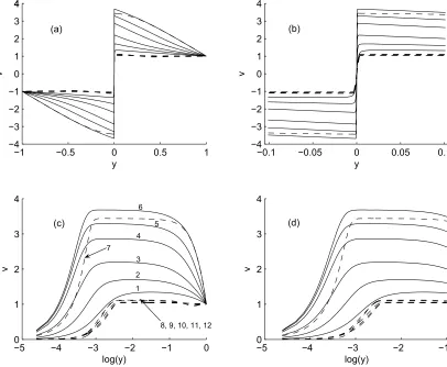
v(0,y) =y, s(0,y) =0, γ(0,y) =0,

í1 í0.5 0 0.5 1

í4

í3

í2

í1 0 1 2 3 4 4

y

v

í0.1 í0.05 0 0.05 0.1

í4

í3

í2

í1 0 1 2 3 4

y

v

í5 í4 í3 í2 í1 0 0

1 2 3 4

log(y)

v

í05 í4 í3 í2 í1 1

2 3 4

log(y)

v

(a) (b)

(c) (d)

1 2 3

5

4 6

7

8, 9, 10, 11, 12

Figure 10: The spatial structure of particle velocity at selected points of time: (a) full linear scale, (c) semi-log scale 0<y<=1, (b) behaviour in the neighbourhood of y=0, linear scale, (d) behaviour in the neighbourhood ofy=0, semi-log scale y>0. The band narrowing stage (the solid curves) includes instants oft= 0.76963(1), 0.77020(2), 0.77056(3), 0.77091(4), 0.77116(5), 0.77145(6) and the band widen-ing or post-localization stage (the dash curves) includes instantst = 0.77254(7), 0.78364(8), 0.78815(9), 0.79408(10), 0.79763(11), 0.80000(12).

The half thickness of the slabHand the nominal strain rate ˙γ0 are taken as 3.47mm and 1000s−1, respectively. Other parameters are

ρ=7860kgm−3, μ=80GPa, κ0=602MPa,

a=6.43×10−4s−1, b=1×104Js2(kgm2)−1, Ψ0=0.017, c=473J(kgoC)−1,

k=49.2J(msoC)−1, m=0.0251, n=0.09. The results presented in this section are obtained with 221 collocation points, the value ofα in the mapping Eq. 43 is 8 andβ in Eq. 17 is 1. The re-sults obtained here are in good qualitative agree-ment with those of Bayliss, Belytschko, Kulka-rni, and Lott-Crumpler (1994), who also stud-ied the sensitivity of the material response to

í5 í4 í3 í2 í1 0 0.8

1 1.2 1.4 1.6 1.8

log(y)

s

í5 í4 í3 í2 í1 0

0 5 10 15 20 25 30

log(y)

plastic strain (

γ

)

í5 í4 í3 í2 í1 0

0 2 4 6 8 10 12

log(y)

θ

í05 í4 í3 í2 í1 0

2000 4000 6000 8000 10000 12000

log(y)

plastic strain rate

(a)

(d) (c)

(b)

1 3 4 5 6

7

8 9 10 12

1 2 3 4 5 6

7

8 9 10 12

7

8, 9, 10, 11, 12

1 2 3 4 5 6

7 8

9 ₁₀

12

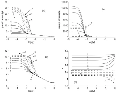
Figure 11: The spatial structure of field variables at selected points of time (a) plastic strain, (b) plastic strain rate, (c) temperature, (d) shear stress. The band narrowing stage (the solid curves) includes instants of

t= 0.76963(1), 0.77020(2), 0.77056(3), 0.77091(4), 0.77116(5), 0.77145(6) and the band widening or post-localization stage (the dash curves) includes instantst= 0.77254(7), 0.78364(8), 0.78815(9), 0.79408(10), 0.79763(11), 0.80000(12).

0.760 0.77 0.78 0.79 0.8 0.81

0.01 0.02 0.03 0.04 0.05

t

1/2 band width

Temperature plastic strain plastic strain rate

0.7692 0.77 0.771 0.772 0.773 0.774

4 6 8 10 12 14x 10

í4

t

1/2 band width

plastic strain rate

(a) (b)

0.74 0.76 0.78 0.8 0.8

1 1.2 1.4 1.6 1.8 2

t

s

0.74 0.76 0.78 0.8

0 5 10 15 20 25

t

plastic strain (

γ

)

0.74 0.76 0.78 0.8

2 4 6 8 10 12

t

θ

0.74 0.76 0.78 0.8

0 2000 4000 6000 8000 10000 12000

t

plastic strain rate

(a) (b)

(c) (d)

t1 t2

t4

t3

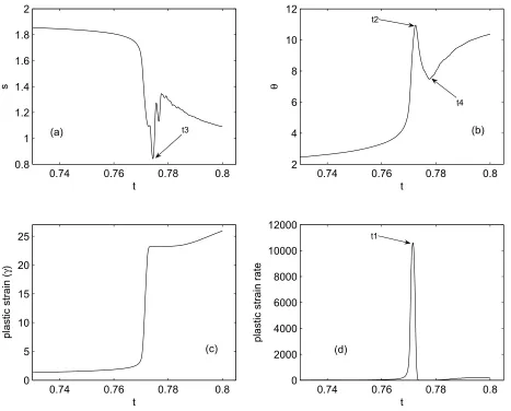
Figure 13: The evolution of (a) shear stress, (b) temperature, (c) plastic strain, (d) plastic strain rate aty= 0. A peak value of the plastic strain rate of 10606.778 occurs att1=0.77154, the temperature of 10.9490 att2=0.77250, the stress of 0.84238 att3=0.77440, and a second peak (local minimum of 7.4781) of temperature att4=0.77759. Thust1<t2<t3<t4.

the field variable profiles are self-similar. The band then widens in the second stage from around time instantt=0.77254 (instant 7) onwards. The bandwidth evolution can be quantified by defining the extent of the bandwidth as the position where the value of a physical property (Θ,γ, or ˙γ) drops to 50% of its value at the band centre (here we use the 50% criterion in order to compare our re-sults with those of Bayliss, Belytschko, Kulkarni, and Lott-Crumpler (1994)). The bandwidths are shown in Figure 12, confirming the band narrow-ing and widennarrow-ing stages as observed above, with the bandwidth for the plastic strain rate being the thinnest and for temperature the thickest. There is

a smooth transitional region between the central shear band and the outer material where the plas-tic strain rate, plasplas-tic strain and temperature pro-files remain virtually unchanged with time. How-ever, the stress profile continues to evolve every-where, with stress level generally dropping due to the softening effect, except some temporary hard-ening at the band centre (Figure 13).

Figure 13 shows the timing of key events dur-ing the process of strain localization. The plas-tic strain rate rises rapidly and attains its peak value at t1 =0.77154, followed by the temper-ature peaking at t2=0.77250, and the stress at

0.76 0.765 0.77 0.775 0.78 0.785

í1

í0.5

0 0.5 1

x 104

t

kθ

,yy dθ/dt plastic work

t1 t2

t3

t4

Figure 14: The interaction between thermal diffusion and plastic heating aty=0: the dash curve depicts the evolution of the effect of thermal diffusion,kΘ_,yy, dash-dot curve the effect of plastic heatingsγ˙, and the

solid curve the combined effect d_dtΘ=kΘ_,yy+sγ˙of thermal diffusion and plastic heating. The onset of strain

localisation occurs att=0.76976. Some key events occur att1=0.77154<t2=0.77250<t3=0.77440<

t4=0.77759, as identified in the previous figure.

in example 1, the onset of localization is found to occur att=0.76976, which is when the rate of temperature increase starts to rise rapidly as shown in Figure 14. This figure also shows that the strength imperfection is such that the ther-mal diffusion process is much slower than the rate of heat generated by plastic work which causes rapid localised increase of Θ. The high temper-ature triggers a dramatic thermal softening pro-cess with a very brief period of elastic unload-ing. Although strain hardening becomes stronger briefly, thermal softening dominates and the band widens. Soon after the onset of localisation, ˙γ aty=0 reaches a peak value ˙γpeak=10606.778

at timet=t1=0.77154 while the strain harden-ing parameter Ψ is still growing. At this time, Θ is still increasing and shear stress decreas-ing. After attaining the maximum value, ˙γ drops rapidly to near zero then rises slowly. There are small oscillations in the behaviour of ˙γ in this regime, which was also found in Bayliss,

Be-lytschko, Kulkarni, and Lott-Crumpler (1994). As the plastic strain rate drops, the rate of plastic heating becomes slower and thermal diffusion be-comes briefly dominant betweent2=0.77250 and

t4=0.77759 when the rate of plastic heating is again faster, causing further temperature rise. At

t=t1=0.77154 the bandwidths are 6.43×10−3, 8.40×10−4_{, 6.75×10}−4_{based onΘ,γ, ˙γ} respec-tively, which are compared with the correspond-ing values of 6.08×10−3, 7.61×10−4, 3.92× 10−4 obtained by Bayliss, Belytschko, Kulkarni, and Lott-Crumpler (1994).

The evolution of plastic strain rate ˙γ, and tem-peratureΘ in the localized region during the se-vere localization are visualised in Figure 15 and Figure 16 respectively. In Figure 17, the evolu-tion of shear stress s over the whole domain is depicted. The spatial profile of the shear stress

ther-í4.6 í4.4 í4.2

í4 í3.8 í3.6

í3.4 í3.2

0.77 0.772 0.774 0.776 1000 2000 3000 4000 5000 6000 7000 8000 9000 10000

log(y) t

plastic strain rate

Figure 15: The evolution of plastic strain rate ˙γ.

í4.5

í4

í3.5

í3

0.77 0.772 0.774 0.776 0.778

5 6 7 8 9 10

log(y) t

θ

Figure 17: The evolution of shear stress.

mal imperfection model considered in example 1 above. The present results are compared with those obtained by the Modified Smooth Particle Hyrodynamics method (MSPH) [Batra and Zhang (2004)] and Chebyshev Pseudo Spectral method (CPS) [Bayliss, Belytschko, Kulkarni, and Lott-Crumpler (1994)] in Tables 1-2. Despite gen-eral qualitative agreement between the methods and some excellent quantitative agreements, there are some large differences between the numeri-cal results. For the timing of key events, t1, t2,

t3,t4, the present results fall between the MSPH and the CPS results and are much closer to the latter (within 7%), although the time lagst2−t1,

t3−t1, t4−t1 are virtually identical between the present IRBFN and the MSPH methods. In con-trast, the results for ˙γpeak, Θpeak, smin, Θmin, γt1

andγt2 are much closer to those obtained by the

MSPH method.

4.3 Convergence characteristics

For example 1, we use six discretisations ({Ni}ip==16 = {61,101,141,181,221,261} uni-formly spaced collocation points, i.e. spacing

hi = 1/Ni) to study the convergence of our

method. Due to a lack of exact solution, an esti-mate of “error" is computed as follows. For each level of discretisation, the governing equations are integrated to a specified time instant just after the onset of localisation (t=60.507μs and

t=0.77115 for example 1 and 2, respectively) to obtain the spatial profile of the temperature at this time instant. Then the temperatures at Q=300 points are computed by interpolation (i.e. by the close form RBFN just found) and the discrete relativeL2error is computed as

Ne=

∑Qj=1(Θij−Θ

p j)2

∑Q j=1(Θ

p j)2

, i=1,2,...,p−1,

where p =6 for example 1 and 5 for example 2. Similarly, for example 2, we use five discreti-sations ({Ni}ip==15 ={61,101,141,181,221} uni-formly spaced collocation points). Figure 18 shows that the “error" is proportional toO(h2.48)

Table 1: Comparison of the results between methods: The results obtained by the present IRBFN method are generally between those by the MSPH and the CPS methods, except for the case ofΘminandγt1.

t1 t2 t3 t4 γ˙peak Θpeak smin Θmin γt1 γt2

MSPH 0.9445 0.9455 0.9474 0.9505 11500 11 0.78 7.4 11 24 IRBFN 0.7715 0.7725 0.7744 0.7776 10606 10.95 0.84 7.48 14.0 22.1

CPS 0.7239 0.7252 0.7268 0.7284 5300 8.61 1.22 6.95 6.8 11.7

Table 2: Comparison of the time lags between methods: agreement is generally excellent, except that the CPS results show an ealier occurrence of the local temperature minimum.

t2−t1 t3−t1 t4−t1 MSPH 0.001 0.0029 0.0060 IRBFN 0.001 0.0029 0.0061 CPS 0.0013 0.0029 0.0045

10í3 10í2 10í1

10í3 10í2 10í1

h

Ne

(a)

10í3 10í2 10í1

10í4 10í3 10í2 10í1

h

Ne

(b)

Figure 18: Convergence characteristics: (a) thermal imperfection model, (b) strength imperfection model.

case of example 2, Bayliss, Belytschko, Kulkarni, and Lott-Crumpler (1994) used 61 points in their CPS method.

5 Conclusion

We use the meshless IRBFN method to analyze the strain localization of an elasto-thermo-visco-plastic slab under simple shearing. We introduce a new coordinate mapping that allows very high resolution of the spatial structure of the resul-tant localised shear band with a relatively small number of computational degrees of freedom, dis-tributed uniformly in the computational domain. The effects of elastic unloading, strain and strain rate hardening, thermal softening, heat conduc-tion are considered. Either the thermal

fur-ther since we are not considering any fracture criterion. The application of the present method to two- and three-dimensional strain localisation problems will be carried out in our future work.

Acknowledgement: This work is supported by the Australian Research Council. This support is gratefully acknowledged.

References

Atluri, S.; Shen, S. (2002): The meshless lo-cal Petrov-Galerkin (MLPG) method:A simple & less-costly alternative to the finite element and the boundary element methods. CMES: Computer Modeling in Engineering & Sciences, vol. 3, pp. 11–51.

Atluri, S. N.; Zhu, T.(1998): A new meshless local Petrov-Galerkin (MLPG) approach in com-putational mechanics. Comput. Mech., vol. 22, pp. 117–127.

Batra, R. C.; Kim, C. H. (1991): Effect of thermal conductivity on the initiation, growth and bandwidth of adiabatic shear bands. Interna-tional Journal of Engineering Science, vol. 29, pp. 949–960.

Batra, R. C.; Zhang, G. M. (2004): Anal-ysis of adiabatic shear bands in elasto-thermo-viscoplastic materials by Modified Smooth-Particle Hydrodynamics (SPH) method. Journal of Computational Physics, vol. 201, pp. 172–190.

Bayliss, A.; Belytschko, T.; Kulkarni, M.; Lott-Crumpler, D. A. (1994): On the dynamics and the role of imperfections for localization in thermo-viscoplastic materials. Modelling and Simulation in Materials Science and Engineering, vol. 2, pp. 941–964.

Hairer, E.; Norsett, S.; Wanner, G. (1987):

Solving Ordinary Differential Equations I. Non-stiff Problems. Springer-Verlag.

Hairer, E.; Wanner, G. (1996): Solv-ing Ordinary Differential Equations II. Stiff and Differential-Algebraic Problems. Springer-Verlag.

Han, Z.; Atluri, S. (2004): A meshless local Petrov-Galerkin (MLPG) approach for 3-diemensional elasto-dynamics. CMC: Comput-ers, Materials and Continua, vol. 1, pp. 129–140.

Han, Z. D.; Atluri, S. N.(2003): Trully Mesh-less Local Petrov-Galerkin (MLPG) Solutions of Traction & Displacement BIEs. CMES: Com-puter Modeling in Engineering & Sciences, vol. 4, no. 6, pp. 665–678.

Han, Z. D.; Liu, H. T.; Rajendran, A. M.; Atluri, S. N.(2006): The Applications of Mesh-less Local Petrov-Galerkin (MLPG) Approaches in High-Speed Impact, Penetration and Perfora-tion Problems. CMES: Computer Modeling in Engineering & Sciences, vol. 14, no. 2, pp. 119– 128.

Han, Z. D.; Rajendran, A. M.; Atluri, S. N. (2005): Meshless Local Petrov-Galerkin (MLPG) Approaches for Solving Nonlinear Prob-lems with Large Deformations and Rotations.

CMES: Computer Modeling in Engineering & Sciences, vol. 10, no. 1, pp. 1–12.

Kansa, E. J.(1990): Multiquadrics – a scattered data approximation scheme with applications to computational fluid dynamics – II. Solutions to parabolic, hyperbolic and elliptic partial differen-tial equations. Computers & Mathematics with Applications, vol. 19, pp. 147–161.

Kansa, E. J.; Power, H.; Fasshauer, G. E.; Ling, L. (2004): A volumetric integral radial basis function method for time-dependent partial differential equations: I formulation. Engineer-ing Analysis with Boundary Elements, vol. 28, pp. 1191–1206.

Li, S.; Liu, W. C. (2000): Numerical simula-tion of Strain localizasimula-tion in inelastic solids us-ing mesh-free method. International Journal for Numerical Methods in Engineering, vol. 48, pp. 1285–1309.

Ling, L.; Trummer, M. R. (2006): Adap-tive multiquadratic collocation for boundary layer problems. Journal of Computational and Applied Mathematics, vol. 188, pp. 265–282.

Madych, W. R.; Nelson, S. A. (1990): Mul-tivariate interpolation and conditionally positive definite functions, II. Mathematics of Compu-tation, vol. 54, pp. 211–230.

Mai-Cao, L.; Tran-Cong, T.(2005): A mesh-less IRBFN-based method for transient problems.

CMES: Computer Modeling in Engineering & Sciences, vol. 7, pp. 149–171.

Mai-Duy, N.(2005): Solving high order ordi-nary differential equations with radial basis func-tion networks. International Journal for Numeri-cal Methods in Engineering, vol. 62, pp. 824–852.

Mai-Duy, N.; Tanner, R. I. (2005): Solving high order partial differential equations with indi-rect radial basis function networks. International Journal for Numerical Methods in Engineering, vol. 63, pp. 1636–1654.

Mai-Duy, N.; Tran-Cong, T.(2001): Numer-ical solution of differential equations using mul-tiquadric radial basic function networks. Neural Networks, vol. 14, pp. 185–199.

Mai-Duy, N.; Tran-Cong, T.(2003): Approxi-mation of function and its derivatives using radial basis function networks. Applied Mathematical Modeling, vol. 27, pp. 197–220.

Mai-Duy, N.; Tran-Cong, T.(2005): An effi-cient indirect RBFN-based method for numerical solution of PDEs. Numerical Methods for Partial Differetial Equations, vol. 21, pp. 770–790.

Mai-Duy, N.; Tran-Cong, T. (2006): Solv-ing biharmonic problems with scattered-point discretization using indirect radial-basis-function networks. Engineering Analysis with Boundary Elements, vol. 30, pp. 77–87.

Molinari, A.; Clifton, R. J.(1987): Analytical characterization of shear localization in thermo-viscoplastic materials. Journal of Applied Me-chanics, vol. 54, pp. 806–812.

Rice, J. R.; Rudnicki, J. W.(1980): A note on some features of the theory of localization of de-formation. International Journal for Solids Stru-crures, vol. 16, pp. 597–605.

Sherif, R. A.; Shawki, T. G. (1992): The role of heat conduction during the post-localization regime in dynamic viscoplasticity. Plastic flow and Creep, ASME, vol. AMD-Vol. 135/MD-Vol. 31, pp. 159–173.

Tang, T.; Trummer, M. R.(1996): Boundary layer resolving pseudospectral methods for singu-lar pertubation problems. SIAM Journal of Sci-entific Computing, vol. 17, pp. 430–438.

Walter, J. W. (1992): Numerical experiments on adiabatic shear band formation in one dimen-sion. International Journal of Plasticity, vol. 8, pp. 657–693.

Wright, T. W.(1990): Adiabatic shear bands.

Journal of Applied Mechanics, vol. 43, pp. S196– S200.

Wright, T. W.(2002): The physics and mathe-matics of adiabatic shear bands. Cambridge Uni-versity Press.