Optic Nerve Head Image Analysis for Glaucoma Progression Detection

(1)

City, University of London Institutional Repository

Citation: O'Leary, Neil (2011). Optic Nerve Head Image Analysis for Glaucoma

Progression Detection. (Unpublished Doctoral thesis, City University London)

This is the unspecified version of the paper.

This version of the publication may differ from the final published

version.

Permanent repository link: http://openaccess.city.ac.uk/1154/

Link to published version:

Copyright and reuse: City Research Online aims to make research

outputs of City, University of London available to a wider audience.

Copyright and Moral Rights remain with the author(s) and/or copyright

holders. URLs from City Research Online may be freely distributed and

linked to.

City Research Online: http://openaccess.city.ac.uk/ [email protected]

(2)

1

Optic Nerve Head Image

Analysis for Glaucoma

Progression Detection

N

EIL

O’L

EARY

PhD Thesis

(3)

2

List of Tables

Table 2.1: The summary of stereophotograph assessment of progression in the study with the proportion of assessments reached by consensus and the proportion requiring adjudication.

74

Table 3.1 Real no-change RA data: the α-level (p-value cut-off) of the hypothesis test of negative change over time for each change detection test given a

fixed/anchored percentage of falsely flagged progressing rim area series at fifth and final examination.

114

Table 3.2 Power levels for three change detection methods of detecting change at

medium trend of RA deterioration (-0.012mm2/year) at 7th visit after 3 years of follow-up in different noise scenarios. Total RA decrease during this follow-up period: 0.036mm2. Entries are colour coded: red corresponds to lower power values, yellow to moderate power values and green to higher power values.

115

high trend of RA deterioration (-0.021mm2_{/year) at 7}th_{visit after 3 years of} follow-up in different noise scenarios. Total RA decrease during this follow-follow-up period: 0.063mm2. Entries are colour coded: red corresponds to lower power values, yellow to moderate power values and green to higher power values.

116

medium trend of RA deterioration (-0.012mm2_{/year) at 13}th_{(and final) visit after 6} years of follow-up in different noise scenarios. Total RA decrease during this follow-up period: 0.072mm2_{. Entries are colour coded: red corresponds to lower} power values, yellow to moderate power values and green to higher power values.

(7)

6

high trend of RA deterioration (-0.021mm2_{/year) at 13}th_{(and final) visit after 6} years of follow-up in different noise scenarios. Total RA decrease during this follow-up period: 0.126mm2_{. Entries are colour coded: red corresponds to lower} power values, yellow to moderate power values and green to higher power values.

118

Table 4.1 Instrument guidelines categorising MPHSD (courtesy of Heidelberg Engineering, Heidelberg, Germany).

131

Table 4.2 Agreement between the subjective assessments of the image quality of HRT mean topography and reflectance image pairs by 6 observers (A – F). Quality assessments were made over a subset of 28 image pairs. Agreement is quantified by use of linearly weighted κ values. Observers were asked to repeat their quality assessments on the same (but reordered) subset (1 – 2). Within observer agreements are in indicated by the italic font. The strength of agreement is indicated by colour - red represents the lowest agreement and green the highest.

154

Table 5.1: Summary of differences (bias and 95% limits of agreement (LoA))

between the simulated and real image series for global, regional and local measures of variability: mean of within examination pixel height standard deviation

(MPHSDw), mean of between examination pixel height standard deviation (MPHSDb), RA CV and NCC of PHSDw. maps.

(8)

7

List of Figures

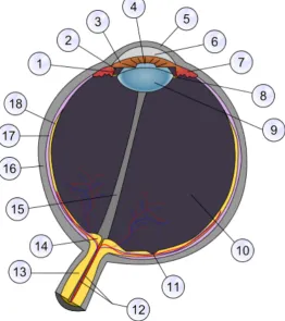
Figure 1.1 Schematic anatomy of the eye. Numbers indicate main or notable features. Important ocular features and those most relevant to glaucoma and ocular imaging include, 2: posterior chamber, 3: iris, 4: pupil, 5: cornea, 6: anterior

chamber (aqueous humour), 9: lens, 10: vitreal chamber (vitreous humour), 11: fovea, 12: retinal blood vessels, 13: optic nerve, 14: optic nerve head or optic disc,

16: sclera, 18: retina.

23

Figure 1.2 Retinal nerve fibre schematics showing (a) exit configurations of retinal nerve fibres leaving the optic nerve head related to the eccentricity of their starting point and (b) the arcuate-path configuration of retinal nerve fibres across the retina. (Images from(Khurana, 2007)

26

Figure 1.2 Schematic of the ONH and optic disc and relationship to the RNFL. 26

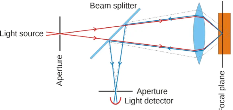
Figure 1.4 Principles of confocal scanning showing the placement of

apertures/pinholes in front of the light source/laser and the detector. With an infinitesimally small aperture any light returning from planes posterior or anterior to the focal plane is rejected.

43

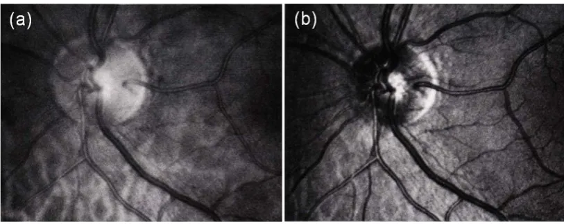
Figure 1.5 Examples of ONH scans of the same eye with a scanning laser

ophthalmoscope system in (a) non-confocal and (b) confocal modes. (Images from (Plesch et al., 1990)

44

Figure 1.6 Principles of CSLT. (a) “Stack” of confocal scanning laser

ophthalmoscope images at incremental focal depths (false colour representation of reflectance intensity). Measurements in the z-axis are referred to as axial and those in the x and y axes are referred to as transverse. (b) The set of axial reflectance values at a given transverse coordinate

_�𝑥

_𝑖

_,

_𝑦

_𝑗

_�

is known as a z-profile. (c) The axial location of each z-profile maximal reflectance at coordinate

�𝑥

𝑖

,

𝑦

𝑗

�

is

calculated and denoted

𝑧

𝑖𝑗. (d) Axial locations are mapped to a topographic height

image. (e) CSLT three-dimensional representation of (d).

(9)

8

Figure 1.7 Comparison of 10° x 10° HRT Classic topography (a) and reflectance images (c) and 15° x 15° HRT II mean topography (b) and mean reflectance images (d). Images have transverse spatial sampling of 256 x 256 (HRT Classic) and 384 x 384 (HRT II) ensuring that transverse spatial sampling intervals are consistent. (Images from Moorfields Eye Hospital clinic database).

47

Figure 1.8 HRT II topography and reflectance images of glaucomatous eye (a) & (c) and normal eye (b) & (d). (Images from Moorfields Eye Hospital clinic database).

48

Figure 1.9 (a) HRT topography with manually delineated optic disc boundary (contour line) and (b) illustration of the derivation of topography optic disc, neuro-retinal rim and cup areas from the reference ring and contour line.

49

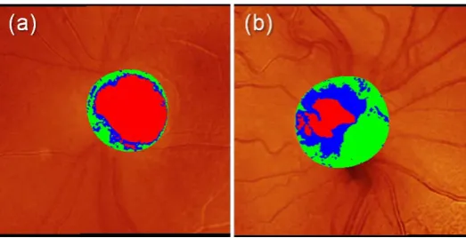
Figure 1.10 HRT II topography images for eyes in Figure 1.8 with overlay of manually delineated optic disc area and colours indicating neuroretinal rim (green and blue) and cup (red). (Images from Moorfields Eye Hospital clinic database).

51

Figure 1.11 Sample HRT Classic topography images series for a sample eye over four visits. TCA outputs are displayed in the top row with statistically significant negative (red) and positive (green) change overlaid. For the same series, overlaid stereometric parameters, rim area and cup area, within the outlined optic disc are shown in the bottom row (colours as per Figure 1.10). A progressive inferior cupping of the optic disc is evident and corresponds with the inferior ‘cluster’ of red pixels in the TCA map. (Images from Moorfields Eye Hospital clinic database)

59

Figure 2.1 Selection criteria applied to stereophotograph and HRT progression study and the resulting sample sizes.

67

Figure 2.2 ROC curves for HRT progression algorithms using stereophotograph-assessed glaucomatous change as the reference standard for TCA, SIM and RALR. Areas under the ROC curves are 0.62 for SIM, 0.61 for TCA and 0.66 for RALR.

75

Figure 2.3 Area proportional Venn diagrams representing the agreement of TCA, SIM and RALR with stereophotograph assessment. Equal rates of identified progression mean that the circles in each diagram are equal in area.

(10)

9

Figure 2.4 Area proportional Venn diagrams representing the agreement of TCA, SIM and ordinary RALR with each other in determining glaucomatous

progression. Equal rates of identified progression mean that the circles are equal in area.

77

Figure 2.5 Case 1. A Single baseline (April 1998) and D single final follow-up (April 2005) photographs from stereophotograph pairs, with excavation and

rim-narrowing indicated supero-temporally and supero-nasally (arrows). B Baseline HRT mean image (April 1998). Final follow-up HRT mean image (April 2005) with C TCA (progression flagged) and E SIM (progression flagged) outputs (the dark red pixels represent the largest cluster of pixels within disc). F Output for RALR (red sectors represent significant p-values for negative trend of RA).

78

Figure 2.6 Case 2. A Single baseline (August 1998) and D single final follow-up (August 2005) photographs from stereophotograph pairs with excavation indicated infero-temporally (arrow). B Baseline HRT mean image (August 1998). Final follow-up HRT mean image (August 2005) with TCA C (no progression flagged) and SIM E (no progression flagged) outputs (dark red pixels represent largest cluster of pixels within disc). F Output for RALR at (red sector and centre represent significant p-value for negative trend of RA).

79

Figure 2.7 Case 3. A Single baseline (October 1998) and D single final follow-up (August 2005) photographs from stereophotograph pairs with excavation indicated infero-temporally (arrow). B Baseline HRT mean image (October 1998). Final follow-up HRT mean image (August 2005) with TCA C (no progression flagged) and SIM E (no progression flagged) outputs (dark red pixels represent largest cluster of pixels within disc). F Output for RALR (green centre represents no significant p-values for negative trend of RA).

80

Figure 2.8 Case 4. A Single baseline (July 1998) and D single final follow-up (July 2005) photographs from stereophotograph pairs with no observed change. B Baseline HRT mean image (July 1998). Final follow-up HRT mean image (July 2005) with TCA C (progression flagged) and SIM E (progression flagged) outputs (dark red pixels represent largest cluster of pixels within disc). F Output for RALR (red

(11)

10

sector and centre represent significant p-value for negative trend of RA).

Figure 3.1 (a) Low, (b) medium and (c) high levels of RA measurement noise

𝜀

_𝑖 with normal, Laplace and hyperbolic probability distributions. Within each level, these distributions have all been adjusted to have equal variances. Shape

parameters of the hyperbolic distributions are consistent with those fitted to observed RA measurement error distributions.

104

Figure 3.2 Box-whisker plots showing the spread of normally distributed

measurement variability at each follow-up examination for stable series. Each panel represents a scenario of measurement variability with the following average magnitudes and its change across the follow-up period: (a) uniform low noise, (b) uniform medium noise, (c) uniform high noise, (d) medium increasing noise, (e) medium decreasing noise, (f) medium noise with an outlier present, and (g) medium noise with autocorrelation.

107

Figure 3.3 Example of ROC curve and the dark grey PAUC within a region of the ROC curve with false positives ≤ 0.2

111

Figure 3.4 (a) HRT Classic data: Percentage of falsely flagged progressing series at fifth and final examination for the p-value cut-off of each change detection test (b) HRT II data: Percentage of falsely flagged progressing series at fifth and final examination for the p-value cut-off of each change detection test.

113

Figure 3.5 Changes with follow-up period of PAUC values (false positive rate < 20%) for the three change detection methods for the three indicated noise distributions in series of a medium trend of RA deterioration (-0.012mm2_/year). The seven scenarios of noise pattern over time are (a) low uniform noise, (b) medium uniform noise, (c) high uniform noise, (d) medium increasing noise, (e) medium decreasing noise, (f) medium noise with an outlier measurement and (g) medium noise with autocorrelation. See Figure 3.2 for illustration of noise patterns.

120

Figure 3.6 Changes with follow-up period of PAUC values (false positive rate < 20%) for the three change detection methods for the three indicated noise distributions in series of a high trend of RA deterioration (-0.021mm2/year). The seven scenarios of noise pattern over time are (a) low uniform noise, (b) medium

(12)

11

uniform noise, (c) high uniform noise, (d) medium increasing noise, (e) medium decreasing noise, (f) medium noise with an outlier measurement and (g) medium noise with autocorrelation. See Figure 3.2 for illustration of noise patterns.

Figure 3.7 Two-hundred randomly sampled permutation distributions of OLS linear regression test-statistics with the parametric Student’s t-distribution (3 degrees of freedom) overlaid for 4 scenarios of noise pattern: (a) medium uniform noise, (b) medium increasing noise, (c) medium noise with an outlier and (d) medium noise with autocorrelation. These distributions are for stable simulated series Laplace measurement noise at 5th_{RA measurement (2 years). The average} p-value for the two-sample Kolmogorov-Smirnov test is for (a) 0.78, (b) 0.81, (c) 0.81 and (d) 0.82.

122

Figure 3.8 Two-hundred randomly sampled permutation distributions of OLS linear regression test-statistics with the parametric Student’s t-distribution (11 degrees of freedom) overlaid for 4 scenarios of noise pattern: (a) medium uniform noise, (b) medium increasing noise, (c) medium noise with an outlier and (d) medium noise with autocorrelation. These distributions are for stable simulated series hyperbolic measurement noise at 13th_{RA measurement (6 years). The} average p-value for the two-sample Kolmogorov-Smirnov test is for (a) 0.52, (b) 0.50, (c) 0.53 and (d) 0.54.

122

Figure 4.1 MRI scans of patient with intractable nocturnal seizures. (a) Coronal image using 1.5-T magnet MRI showing questionable curvilinear focus of high signal intensity (arrows). Abnormal signal intensity was missed at first review of images. (b) Coronal image using 3-T MRI showing curvilinear band of high signal intensity (arrows) white matter without apparent mass effect. (Reproduced from (Phal et al., 2008))

129

Figure 4.2 Example output of image quality assessment by HRT software of the constituent images in a HRT mean topography.

130

Figure 4.3 Sample mean topographies (a) and (d) with respective PHSD maps (b) and (e). PHSD distributions (c), (f) are also displayed. MPHSD values are 15µm and 30µm for (a) and (b) respectively.

(13)

12

Figure 4.4 Sample HRT Classic topography displayed in three dimensions with reflectance intensity colour mapping. Misalignments due to translations

�𝑡𝑥

,

𝑡𝑦

,

𝑡𝑧�

along and rotations

(

∅

,

𝜌

,

𝜃

)

about the

(

𝑥

,

𝑦

,

𝑧

)

axes are shown. Measurements and translations in the

𝑧

-axis are referred to as axial and those in the

𝑥𝑦

plane as transverse.

137

Figure 4.5 The simulation schematic with three different, random misalignment and noise sets applied to a seed single topography to produce three simulated single topographies for two sample eyes. In this example each set applied is

identical for both eyes and this is the case across all seed topographies in the analysis.

139

Figure 4.6 The relationship of MPHSD of a 256 x 256 ‘flat’ image with different levels of morphologically independent noise added. Boundary points where MPHSD values are produced corresponding with the minimum MPHSD observed in real data (10µm) are indicated.

140

Figure 4.7 Fourier analysis example of (a) an image with periodic vertical stripes, (b) photograph of Pádraig Mac Piarais in side profile, (c) telescope image of the M91 galaxy, (d) power spectrum of (a), (e) power spectrum of (b), (f) power spectrum of (c). The brighter the points in (d), (e) and (f) indicate the higher amplitude of a given frequency - lower frequencies are located towards the centre of these images and higher frequencies towards the edges. Note that log scales for the intensity are used for (d), (e) and (f) as the proportions of frequency

components at the centre (representing the average of the signal) and at key characteristic frequencies are much higher than elsewhere.

143

Figure 4.8 Fourier analysis, example of (a) single topography image, (b) single reflectance image, (c) magnitude of frequency spectrum of single topography image, (d) magnitude of frequency spectrum of single reflectance image, (e) RASD (dashed lines) with solid vertical lines representing the centroid for the reflectance and topography images. The position of each RASD centroid is also marked on images (c) and (d).

(14)

13

Figure 4.9 Gradient analysis, example of (a) mean real topography PHSD map, (b) mean simulated topography PHSD map, (c) average GM map of constituent real single topography images, (d) GM map of seed single topography image, (e) average GM map of constituent real single reflectance images. For real data, cross-correlation coefficients are 0.41 between maps (a) and (c) and 0.25 between maps (a) and (e). For simulated data, cross-correlation coefficients are 0.64 between maps (b) and (d). Note: Grey-scale maps have equal ranges across rows of this Figure but not along columns.

146

Figure 4.10 (a) Distribution of the MPHSD values for all 74 HRT Classic baseline mean topographies. (b) Distribution of the MPHSD values for a subset of 28 randomly selected topographies from all 74 HRT Classic mean topographies.

148

Figure 4.11 MPHSD values compared to inter-quartile range (IQR) values for PHSD distributions.

149

Figure 4.12 (a) Series RA standard deviation values plotted against series-averaged MPHSD values. (b) The magnitude of difference of individual RA measurements from the series RA best available estimator (BAE) - as calculated by the series average RA measurements – as a fraction of series RA standard deviation plotted against MPHSD values as a fraction of series-averaged MPHSD values. Areas of a higher density of points are represented by darker shading.

150

Figure 4.13 MPHSD values for real and simulated mean topographies. The

minimum observed MPHSD (10µm) in real mean topographies is plotted as a lower bound for simulated mean topography MPHSD. Pearson’s sample correlation coefficient

_𝑟

: 0.79 (p<0.001), MPHSD real – MPHSD simulated mean: 7.6 µm, standard deviation: 13.7 µm.

151

Figure 4.14 Fourier metrics of constituent single images compared to MPHSD values. Pearson’s

_𝑟

correlation coefficients are for (a) 0.74, (b) 0.93, (c) 0.69, (d) -0.55, (e) 0.58 and (f) 0.58.

152

Figure 4.15 Measure of the average GM of constituent single images compared to MPHSD values. Pearson’s

_𝑟

correlation coefficients are for (a) 0.95, (b) -0.51 and (c)

(15)

14

0.85.

Figure 4.16 Distributions of (a) averaged measure of the NCC of real mean topography PHSD maps and GM maps for each constituent single topography (b) averaged measure of the NCC of real mean topography PHSD maps and GM maps for each constituent single reflectance image and (c) averaged measure of the NCC of multiple simulated mean topography PHSD maps and GM maps for single seed topographies. Means of distributions are 0.375, 0.25 and 0.56 for (a), (b) and (c) respectively.

153

Figure 4.17 Subjective observer assessed panel scores of image quality of mean topography and reflectance image pairs compared to (a) MPHSD, (b)

reflectance/topography image combined RASD centroid measurement and (c) reflectance/topography image combined mean GM. Coloured points on figures

correspond to those examples in Figure 4.18. Pearson’s

𝑟

correlation coefficients are for (a) 0.81 (b) 0.81 and (c) 0.28.

155

Figure 4.18 Examples of reflectance-topography image pairs (a)-(b), (c)-(d), (e)-(f) and (g)-(h) presented to experienced Heidelberg Retina Tomograph operators with mean panel scores (rounded to nearest category) and standard deviation of scores across all observers. MPHSD values and manufacturer supplied categories for these values are displayed. Coloured symbols are used to represent these examples in Figure 4.15. (SD: standard deviation).

156

Figure 5.1 Schematic of simulation: HRT single and mean topography formation formed from a single scan volume of CSLO optical sections. Processes are

represented by grey boxes with intermediate data states by white boxes and initial and final data states by rounded boxes.

167

Figure 5.2 Bland-Altman plots showing series-wise, agreements between (a) average within examination MPHSD (MPHSDw) for real and simulated mean topography data and (b) agreement of between examination (MPHSDb) for real and simulated mean topography data. The mean difference (bias) of average MPHSDw is 3.5µm (95% limits of agreement: -20.9µm to 28.8µm). The mean difference of MPHSDb is 2.0µm (95% limits of agreement (LoA): -5.4µm to 9.3µm). Uniform 95%

(16)

15

LoA illustrate only approximate limits of agreement as heteroscedasticity of this data is apparent.Dashed lines indicate statistically significant linear proportional bias for MPHSDb and the significant linear proportional increase of the widths of the 95% LoA for MPHSDw and for MPHSDb.

Figure 5.3 Bland-Altman plots showing series-wise agreement between RA CV for real and simulated data (%). Mean difference between values for real and simulated data is -2.1% (95% limits of agreement (LoA): -17.6% to 13.4%). No proportional effects are found on the bias or LoA.

179

Figure 5.4 Distributions of maximal NCC of pixel standard deviation maps

between real and simulated data (a) within examination (PHSDw) averaged over all pair-wise comparisons and (b) between examination (PHSDb). (c) The series

average NCC values of all pair-wise pixel standard deviation maps between mean topographies in the same series. Value extremes are interpreted as follows: -1: perfectly negatively correlated, 0: uncorrelated, 1: perfectly positively correlated.

180

Figure 5.5 Benchmarking of PHSDw NCC values between real and simulated data: Bland-Altman plot showing agreement of average NCC for real/real PHSDw map comparisons and average NCC for real/simulated PHSDw map comparisons. Solid lines represent a uniform bias of 0.052 and 95% limits of agreement of 0.039 to 0.065. The dashed line represents the statistically significant linear proportional bias.

181

Figure 5.6 Qualitative display of within examination, local variability for real and simulated pairs. (a) Real mean reflectance image. (b) Corresponding simulated mean reflectance image. (c) Real mean topography (mean of within examination pixel height standard deviation (MPHSDw) 20µm). (d) Corresponding simulated mean topography (MPHSDw 22µm). (e) Log of pixel height standard deviation (PHSDw) maps of real mean topography – darker areas represent areas of higher variability. (f) Log of PHSDw maps of corresponding simulated mean topography. Maximal normalised cross correlation of these two maps (e) and (f) is 0.55.

182

(17)

16

Figure 5.7 Qualitative display of within examination, local variability for real and simulated pairs. (a) Real mean reflectance image. (b) Corresponding simulated mean reflectance image. (c) Real mean topography (mean of within examination pixel height standard deviation (MPHSDw) 17µm). (d) Corresponding simulated mean topography (MPHSDw 16µm). (e) Log of PHSDw maps of real mean topography - darker areas represent areas of higher variability. (f) Log of PHSDw maps of corresponding simulated mean topography. Maximal normalised cross correlation of these two maps (e) and (f) is 0.37.

Figure 5.8 Qualitative display of between examination, local variability for real and simulated pairs. (a) Real series-average mean reflectance image. (b) Corresponding simulated series-average mean reflectance image. (c) Real series-average mean topography (mean of between examination pixel height standard deviation (MPHSDb) 39µm). (d) Corresponding simulated series-average mean topography (MPHSDb 38µm). (e) Log of PHSDb maps of real mean topography series - darker areas represent areas of higher variability. (f) Log of PHSDb maps of corresponding simulated mean topography series. Maximal normalised cross correlation of these two maps (e) and (f) is 0.51.

184

Figure 5.9 Qualitative display of between examination, local variability for real and simulated pairs. (a) Real series-average mean reflectance image. (b) Corresponding simulated series-average mean reflectance image. (c) Real series-average mean topography (mean of between examination pixel height standard deviation (MPHSDb) 9µm). (d) Corresponding simulated series-average mean topography (MPHSDb 9µm). (e) Log of PHSDb maps of real mean topography series - darker areas represent areas of higher variability. (f) Log of PHSDb maps of corresponding simulated mean topography series. Maximal normalised cross correlation of these two maps (e) and (f) is 0.73.

(18)

17

Acknowledgements

This thesis would not have been possible without the guidance, inspiration and

encouragement of my supervisors, Professor David Crabb and Professor David

Garway-Heath, who have been so generous with their time and moved me to seek

interesting research questions. I would also like to thank Dr. Tuan Ho for his

unselfish support and advice.

I would like to acknowledge that my PhD benefited from being registered as a

visiting research fellow at the glaucoma research unit in Moorfields Eye Hospital

where I was able to receive further guidance at research meetings. Furthermore, the

generous and unrestricted bursaries and awards from Moorfields Eye Hospital

Special Trustees, Heidelberg Engineering, City University and the Worshipful

Company of Lightmongers supported my research, attendance at international

conferences and publication costs over a four year period.

I would also like to heartily thank my friends and colleagues at City University and

Moorfields Eye Hospital for the many discussions and helpful feedback and for

making my time in London a happy one.

Finally I thank my parents, family and Neasa for their unwavering support and

love throughout all my studies.

(19)

18

Declaration

This thesis has been completed solely by the candidate, Neil O’Leary. It has not

been submitted for any other degrees, either now or in the past. Where work

contained has been previously published, this has been stated in the text. This

grants powers of discretion to the University Librarian to allow the thesis to be

copied in whole or in part without further reference to the author. This permission

covers only single copies made for study purposes, subject to normal conditions of

(20)

(21)

20

Abstract

Glaucoma is a leading cause of visual disability across the world and when

diagnosed the glaucoma patient will spend the rest of their life receiving treatment in managed clinical care. In the glaucoma clinic, retinal and optic nerve head (ONH) imaging can be used to help the clinician to manage patient treatment

appropriately. By providing high resolution images of the optic nerve head

structures and identifying changes therein related to disease onset and progression, an objective measure can be obtained as to how well or badly treatment is

preventing further disease damage. This thesis contributes to the field of glaucoma progression detection by the analysis of clinical imaging data using confocal scanning laser tomography (CSLT). Primarily it is an investigation of how best to appraise and optimise current algorithms which aim to detect these glaucomatous structural changes in the optic nerve head. This is done by addressing how the performance of these methods can be best assessed in the absence of a gold standard for glaucomatous structural progression.

Glaucoma expert assessment of photographs of the optic disc is the current clinical standard of assessing glaucomatous damage evident in the ONH. This is used in this thesis to act as a reference standard by which these algorithms can be

compared. In addition, the statistical principles underpinning trend detection techniques are also investigated along with the performance of these techniques to detect trends in CSLT data in the presence of different types of measurement noise and image quality. A new computer model is developed and validated to simulate stable series of CSLT images, with realistic variability, which can be used to

(22)

21

List of Abbreviations and

Terms

α-level AGIS AUC CSLO CSLT CSM CV GM HRT IOP MRI MPHSD NCC NTG OCT OHT OLS ONH P-DIST PAUC PHSD Power RA RALR RASD RGC ROC RHO P-DIST SIM SLO SLP T-DIST TCA

statistical significance level (p-value cut-off) Advanced glaucoma intervention study

Area under the receiver operating characteristic curve Confocal scanning laser ophthalmoscopy

Confocal scanning laser tomography Cup shape measure

Coefficient of variation Gradient magnitude

Heidelberg retina tomograph Intraocular pressure

Magnetic resonance imaging

Mean pixel height standard deviation Normalised cross-correlation

Normal tension glaucoma Optical coherence tomography Ocular hypertension

Ordinary least squares Optic nerve head

Permutation distribution

Partial area under the partial receiver operating characteristic curve Pixel height standard deviation

Probability of detecting change at a given level of statistical significance

Neuroretinal rim area Rim area linear regression

Radial-averaged spectrum density Retinal ganglion cell

Receiver operating characteristic

Permutation distribution of Spearman’s rank correlation coefficient Statistic image mapping

(23)

22

1. Background and Aims

This chapter gives an introduction to glaucoma, a brief description of its nature,

prevalence and its risk factors. The clinical means to detect and monitor this disease

are discussed. Confocal scanning laser tomography, the focus of this thesis, is

introduced as a technology which can contribute to clinical decision making by

assisting in glaucoma detecting and monitoring.

1.1 Glaucoma

The glaucomas are a group of optic neuropathies, collectively referred to as

glaucoma, that have in common a progressive degeneration of retinal ganglion cells

(RGC) and their axons. They result in distinct damage to the optic nerve head

(ONH) and peripheral vision loss. The mechanism of this RGC degeneration is

intrinsically linked with intraocular pressure (IOP) and often associated with

increased IOP. Glaucoma leads to distinctive changes in the shape or morphology of

the ONH (Figure 1.1) called ‘cupping’. This damage to the ONH causes losses to the

visual field, which is “that portion of space in which objects are simultaneously

visible in the steadily fixating eye” (Spector, 1990). The resulting damage to the

visual field is irreversible; though loss can be transitory in the early stages of

glaucoma. If untreated, the damage to the affected visual field will most likely

intensify and spread until eventually complete loss of vision can occur. It has been

estimated that in the year 2000 that at least 67 million people suffered from

glaucoma with an a resulting estimated 7 million suffering blindness in both eyes

(Quigley, 1996), making it the second leading cause of world blindness (Resnikoff et

(24)

23

longevity of the population, an increased figure of 80 million has been predicted for

2020 with 11 million cases of blindness from glaucoma (Quigley and Broman, 2006).

Furthermore, as the World Health Organisation’s definition of blindness is based on

central vision loss only, the disabling effects of peripheral vision loss are often

under-estimated until later stages of the disease have been reached (Quigley, 1996).

There is no cure for glaucoma but once detected, appropriate clinical intervention

and treatment can help to slow further progression of vision loss – sight cannot be

restored but may be maintained making earlier detection all the more important.

Our understanding of the causes, mechanisms and manifestations of glaucomatous

damage has been shaped by what is measured and how these measurements are

made. Currently three measured features are considered crucial to the recognition of

glaucoma, the ONH, the visual field and IOP. Previously it was believed that

glaucoma was caused solely by elevated IOP and definitions for glaucoma

historically relied on this belief. ‘Normal’ IOP was defined as that which was within

2 standard deviations of the mean IOP found in the general population of 15.5

mmHg (Colton and Ederer, 1980). Ocular hypertension (OHT) is a condition in

which IOP is above this upper limit (greater than 21 mmHg) and historically it

became mistakenly synonymous with pre-glaucoma or glaucoma without damage

(Phelps, 1977). The association between OHT and glaucoma is now known to be

multi-factorial and complex. The prevalence of OHT patients with glaucomatous

visual field damage has been reported as approximately 10% (Sommer et al., 1991),

though an increased prevalence of glaucoma was shown with increased IOP. In

addition, an estimated 10% of untreated OHT patients developed glaucomatous

optic nerve or visual field damage within an average follow-up period of 5 years

(Kass et al., 2002). It is now understood that glaucoma can occur in eyes with

(25)

24

glaucomatous damage and that some eyes are more susceptible to the effects of IOP

and sustain damage at a lower level. Still, as IOP is the only treatable risk factor for

[image:25.595.191.454.155.451.2]

glaucoma, the reduction of IOP remains central to glaucoma treatment.

Figure 1.1 Schematic anatomy of the eye. Numbers indicate main or notable

features. Important ocular features and those most relevant to glaucoma and ocular

imaging include, 2: posterior chamber, 3: iris, 4: pupil, 5: cornea, 6: anterior chamber

(aqueous humour), 9: lens, 10: vitreal chamber (vitreous humour), 11: fovea, 12:

central retinal blood vessels, 13: optic nerve, 14: optic nerve head or optic disc, 16:

sclera, 18: retina. (Public domain image from http://commons.wikimedia.org [User:

Rhcastillhos])

To understand IOP and its importance in glaucoma, it is crucial to consider the

dynamics of the aqueous humour, the clear watery fluid secreted into the posterior

chamber that circulates through the anterior chamber (Figure 1.1). This fluid is

(26)

25

contained in the rear chamber. The function of aqueous humour is to supply

nutrients to the lens and cornea, dispose of the eye's metabolic waste and help

maintain eye shape by regulating IOP. To maintain an IOP the inflow of newly

produced aqueous humour is balanced by an outflow by drainage between the iris

and cornea (Figure 1.1), primarily (80-90%) through a sponge like substance known

as the trabecular meshwork, the remaining fluid outflow occurs independently

through uveoscleral drainage.

Glaucoma is also better understood once the basic principles have been established

of how the eye receives and converts light information into neuronal signals to send

to the brain. As light enters the eye, it is transmitted and refracted to the retina

where it stimulates two different types of photoreceptor cells, called cones and rods,

which produce electrical signals when activated. Rods become active at low levels of

illuminance while cones are active at high levels and so enable human vision to

operate over a wide range of stimulus intensities. The RGCs process the signals

from these photoreceptors before refining and relaying them to the brain through

their axons which exit the eye via the ONH. In humans there are over a million

RGCs. The centre of the retina (macula) has a higher concentration of RGCs and

cones, where vision resolution is best (Rabbetts, 1998, Purves, 2004). These axons

comprise the innermost layer of the retinal nerve fibre layer (RNFL). In mammals

the axons of RGCs are guided to the ONH during embryonic development in a

process called pathfinding (Oster et al., 2004). These axons converge on the ONH

and exit the eye to the brain, passing through the lamina cribrosa - a mesh-like

structure of collagen fibres (Figure 1.2). This convergence and exit forms the

papillary structure of the ONH consisting of a rim of neural tissue and a central

(27)

[image:27.595.114.545.367.586.2]

26

Figure 1.2 Retinal nerve fibre schematics showing (a) exit configurations of retinal

nerve fibres leaving the optic nerve head related to the eccentricity of their starting

point and (b) the arcuate-path configuration of retinal nerve fibres across the retina.

(Images from(Khurana, 2007)

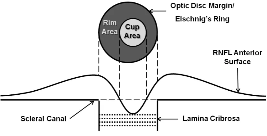
Figure 1.3 Schematic of the ONH and optic disc and relationship to the RNFL.

Glaucoma can be divided into various sub-categories depending on its aetiology

and the mechanism of damage (Allingham and Shields, 2005). Glaucoma is defined

as secondary or primary depending on whether the glaucoma is associated with

(28)

27

be broadly categorised further into open-angle glaucoma, closed-angle glaucoma or

congenital. Primary open angle glaucoma (POAG) and primary closed angle

glaucoma (CAG) are the most prevalent of the glaucomas and their descriptions will

follow. Normal tension glaucoma (NTG) is a subdivision of POAG and is

characterised by an IOP equal to or below 21 mmHg and thus POAG and NTG

appear to represent a continuum of glaucomas with considerable overlap of

causative factors. Outside Japan, more than 30% of newly diagnosed cases are NTG

(Sommer et al., 1991, Dielemans et al., 1994, Mitchell et al., 1996). The condition may

be under-diagnosed in Western countries because of the nature of case-finding for

glaucoma. In Japan NTG is the most prevalent form of Glaucoma (Shiose et al.,

1991). In CAG the iris is pushed against the trabecular meshwork, sometimes

sticking to it and closing off the drainage angle. This angle closure can be an acute

condition - occurring abruptly and resulting in a large and sudden rise in IOP. CAG

may account for up to 50% of glaucoma worldwide as it has a higher prevalence

amongst Asians. Congenital glaucoma is a rare glaucoma typically characterised by

the improper development and consequent dysfunction of the eye's aqueous

drainage channels.

This thesis focuses on POAG; The 2010 American Academy of Ophthalmology

Preferred Practice Pattern (American Academy of Ophthalmology Glaucoma Panel,

2010) defines POAG as “a chronic ocular disease process that is progressive,

generally bilateral, but often asymmetric.” According to their guidelines, it is

associated with the following characteristics:

1) Evidence of optic nerve damage from either, or both, of the following:

(29)

28

b) Reliable and reproducible visual field abnormalities considered a valid

representation of the subject's functional status

2) Adult onset

3) Open anterior chamber angles

4) Absence of other known explanations (i.e., secondary glaucoma) for progressive

glaucomatous optic nerve change

POAG is the most common form of glaucoma in European, African and North

American populations and the second most common form in Asia. To summarise

recent studies the prevalence was reported at 1.5-2.4% in Caucasians, 6-8% in

Afro-Caribbean’s and 1.7-2.0% in Chinese populations (Tielsch et al., 1991, Klein et al.,

1992, Coffey et al., 1993, Dielemans et al., 1994, Leske et al., 1994, Mitchell et al.,

1996, Wolfs et al., 2000, Foster et al., 2000, Friedman et al., 2004b, Wang et al., 2010).

Whereas CAG is often an acute disease, POAG is normally a chronic disease,

resulting in slow progressive damage to the ONH and deterioration of the visual

field.

The debilitating effects of glaucoma in everyday visual function are worth

considering in light of its prevalence. Though central vision is preserved until the

latter stages glaucoma, there is emerging evidence that glaucomatous patients, even

with relatively modest visual field defects, may be at increased risk of falls and

accidents (Turano et al., 1999, Szlyk et al., 2005, Haymes et al., 2007, Ramulu, 2009).

It has also been reported that glaucomatous field defects impact self-assessed

disability (Nelson et al., 2003, Noe et al., 2003) and, more recently, objective

measures of performance in laboratory-based studies have shown the difficulty

(30)

29

Glaucoma will affect an individual’s quality of life when visual field loss makes an

individual unable to drive safely, and several studies of varying experimental

design have shown that certain glaucomatous visual field defects are not compatible

with safe driving (Johnson and Keltner, 1983, McGwin et al., 2004, Haymes et al.,

2007, Haymes et al., 2008). These considerations make understanding glaucoma

with a view to detecting and treating glaucoma earlier even more compelling.

Glaucomatous neuropathy preferentially damages RGC axons at the vertical poles

of the ONH and is influenced to a variable extent by the level of IOP. Though RGC

death occurs by apoptosis, the pathogenesis of this is not wholly understood.

Underlying theories for axonal loss can be can be grouped by mechanisms of direct

mechanical effects or those which are vascular related - through ischemia. These

mechanisms are believed to act in combination rather than one acting at the

exclusion of the other. The mechanicaltheorysuggests that IOP acts directly on the

lamina cribrosa and, as axons leave the eye through its complex connective tissue, a

resulting shearing force is applied. This force causes either direct damage to the

axons or disruption to the transportation of neurotrophic factors (Quigley and

Addicks, 1980) necessary for survival, can lead to morphological changes in the

RGC such as shrinking (Morgan, 2002) and eventually to the death of the cell

(Crawford et al., 2000). The lamina cribrosa is less well supported at its inferior and

superior margins, offering an explanation for the characteristic damage seen in

glaucoma in these locations (Quigley and Addicks, 1981). Furthermore, animal

models of short-term IOP increase show corresponding increased pressure

gradients across the lamina cribrosa. Histology has shown the laminar structure is

not restored to its original state when the IOP is reduced (plastic deformation) and

that this structure becomes more easily deformed at the re-application of increased

(31)

30

can affect blood flow in the ONH may also be a factor in glaucomatous damage.

Changes within the microcirculation of the ONH capillaries are responsible for

axonal loss. Glaucomatous damage can be greater in eyes when the difference

between systemic blood pressure and IOP (perfusion pressure) is low (Sommer, 1996).

Perfusion pressure is an important determinant of ocular blood flow (Hayreh, 2001)

and it has been reported to be lower in POAG patients than in OHT patients when

other factors were controlled (Kerr et al., 1998). In glaucoma, RGC apoptosis and

loss of axons, along with the deformation of the lamina cribrosa leads to

characteristic morphological changes of the ONH. Neuroretinal rim decreases in

size (narrowing its surface area) with parallel enlargement of the cup (widening its

surface area) and thus these morphological changes are of particular interest for

evaluating disease state.

The term optic disc is often used interchangeably with ONH but in this thesis, to help

with clarity, it is used to refer to the anterior surface and anterior features of the

ONH or that portion of the ONH which is clinically visible by ophthalmoscopy

(Jonas et al., 1999). Understanding the features of the optic disc (Figure 1.3) is

important for glaucoma assessment. Optic disc area and relative rim area have large

between-individual variation. This physiological variability makes glaucoma

identification from these features alone difficult. A healthy neuroretinal rim is

typically widest in the inferior optic disc region, and then in the superior, nasal and

finally temporal regions, termed the ‘ISNT’ rule (Jonas and Garway-Heath, 2000).

As outlined, glaucomatous damage to the rim is more or less likely in different

regions and this depends on the stage of the disease. Most frequently, the disease

starts with loss in the inferotemporal and superotemporal regions, followed by the

temporal region and lastly in the nasal region (Hitchings and Spaeth, 1977,

(32)

31

associated with the disease (Drance, 1989) and occur in about 4-7% of glaucomatous

eyes. This occurrence is not useful for identifying glaucoma alone due to their

occurrence in other optic nerve diseases such as drusen (Hitchings et al., 1976).

Diffuse or localised loss of RNFL occurring in glaucoma can also be evident as

visible defects in the RNFL which are not present in healthy eyes (Quigley et al.,

1992, Jonas and Schiro, 1994). Other features such as vascular changes, peripapillary

atrophy and optic disc pallor are also associated with glaucoma. Therefore,

examination of the optic disc and surrounding regions is of importance in both

diagnosis and detection of progressive damage as will be discussed further.

Risk factors are factors which predispose an individual to disease and are clinically

useful to assess the risk of POAG based on the unique characteristics of the patient.

POAG risk factors can be separated along demographic and clinical lines though it

is likely that a combination of factors increase an individual’s risk. It is worth noting

that the appearance of the optic disc is not considered a risk factor because its

characteristics are part of the definition of glaucoma. Many risk factors have been

identified but only a smaller number have strong evidential support (Friedman et

al., 2004a). One of the strongest risk factors is elevated IOP, and several studies have

demonstrated that the prevalence of POAG increases progressively with higher

levels of IOP (Pohjanpelto and Plava, 1974, Sommer et al., 1991). It has been

suggested that the overall risk of developing POAG is five times higher with IOP>21

mmHg (Leske, 1983). More recently, a large population study of OHT patients

showed higher baseline IOP to remain a leading risk factor for development of

POAG (Gordon et al., 2002). Population-based studies of prevalence and incidence

of POAG have shown consistently that age is one of the most important risk factors

(Tielsch et al., 1991, Klein et al., 1992, Coffey et al., 1993, Dielemans et al., 1994,

(33)

32

these studies reported prevalence rates roughly doubling for each decade after 40.

Studies into racial risk factors show that being of African, African-American or

Afro-Caribbean origin puts one at a four-fold increased risk of developing POAG

over white patients when averaged across age groups (Tielsch et al., 1991, Leske et

al., 2004, Girkin, 2004a). Less data are available regarding POAG in other racial

groups though results suggest that those from the Indian sub-continent have higher

prevalence rates (Ramakrishnan et al., 2003), while those of Hispanic origin likely

have intermediate prevalence of POAG between those of African descent and

whites (Quigley et al., 2001).

A positive family history of the disease also gives an individual a higher risk of

developing POAG, though the disease does not usually exhibit Mendelian

inheritance. Studies in families with and without cases of glaucoma led to the

conclusion that IOP and the aqueous outflow facility are multi-factorial in

determination and that POAG is probably multi-factorial also (Armaly, 1968).

Evidence of a genetic background comes from studies indicating that the prevalence

of POAG in first-degree relatives of POAG patients is 7-10 times higher than in the

general population (Becker et al., 1960, Perkins, 1974). There is also a high

concordance rate for POAG between monozygotic twins (Goldschmidt, 1973). More

recent advances in genetics have led to the mapping of glaucoma genes, however,

these genes only account for a small portion of diagnosed glaucoma: a mutation in

one of these genes, labelled MYOC, is found in 3-5% of late-onset POAG (Stone et

al., 1997). Ethnic risk factors are also significant as has been discussed.

Further risk factors for POAG include myopia and diabetes (Leske, 1983, Wilson et

al., 1987), while another study reports a relationship between elevated blood

(34)

33

glaucoma can be found in (Allingham and Shields, 2005). As IOP is the only

treatable risk factor with strong evidence, most treatments of glaucoma focus on

reducing IOP and its fluctuation. As glaucomatous neuropathy cannot be reversed,

and due to the chronic nature of POAG, treatments can often be considered within

the overall context of disease management. Treatments can be broken down into

medication, laser surgery and incisional surgery.

The management of POAG usually involves some form of topical and occasionally

orally administered treatments that enhance aqueous outflow or reduce aqueous

production or both. Prostaglandin analogues are the most commonly prescribed

medication for glaucoma and work by increasing uveoscleral outflow (Allingham

and Shields, 2005), beta-blockers inhibit aqueous secretion and were commonly

used in initial medical management but their use in has declined recently in favour

of prostaglandin analogues. Other treatments such as cholinergic agents cause

ciliary muscle contraction which stretches the trabecular meshwork (Krieglstein,

2000), carbonic anhydrase inhibitors inhibit aqueous production, adrenergic

agonists also inhibit aqueous production and increase trabecular outflow

(Allingham and Shields, 2005). As the actions of the various groups of drugs are

different, combinations of these agents can be applied to achieve a target IOP.

Topical medicines containing combinations of treatments are often prescribed to

patients who require more than one type of drug for control of their glaucoma. This

can help to reduce the burden of self-administered treatment on the patient. These

treatments, in isolation or combined with others, have side effects (local to the eye

and systemic) of varying severity (Detry-Morel, 2006). The overriding goal of

medical treatment is to use the least number of medications necessary to achieve a

(35)

34

Laser surgery targeting the trabecular meshwork is known as trabeculoplasty. The

two most common methods, Argon laser trabeculoplasty and the newer procedure

selective laser trabeculoplasty both reduce IOP by improving aqueous humour

outflow and differ in the type of laser used. Both treatments apply laser energy,

usually to one half of the angle of the trabecular meshwork at a time. Selective laser

trabeculoplasty is a potentially repeatable procedure because of the lack of

coagulation damage to the trabecular meshwork, as shown in one study (Kramer

and Noecker, 2001). Both treatments are simple, cost-effective and, once performed,

do not depend on the compliance of the patient to self-administer medication. Laser

trabeculoplasty has been shown to be at least as effective as medical treatment (The

Glaucoma Laser Trial Research Group, 1990). Other studies have shown that the

effects of laser trabeculoplasty are not always long-lasting however; IOP tends to

rise over time in many patients (Schwartz et al., 1985).

The most common incisional surgery performed in adults for glaucoma is

trabeculectomy. This filtering procedure involves the removal of small part of the

trabecular meshwork, specifically of a block of limbal tissue beneath the scleral flap.

This creates a passageway for aqueous to escape from inside the anterior chamber of

the eye to a pocket created between the conjunctiva and the sclera. Studies have

shown trabeculectomy to be more effective than medical and laser treatments at

lowering IOP and in preserving visual function in the long-term (Burr et al., 2005).

Other surgical techniques, tube-shunt surgery or drainage implant surgery involve

the placement of a tube or glaucoma valves to facilitate aqueous outflow from the

anterior chamber. Laser and incisional surgeries carry with them low but significant

rates of adverse risks such as infection, post-operative transient IOP increases,

(36)

35

(Allingham and Shields, 2005). In the last decade some clinical trials have reported

on the effects of treatment over long term patient follow-up.

The Early Manifest Glaucoma Trial (Heijl et al., 2002) compared the effects of

lowering IOP using trabeculoplasty combined with medical treatment against no

treatment or later treatment. The study showed treatment significantly delays

further visual field deterioration with rates of detected further visual field

deterioration of 41% in the treated group and 51% in the other group in a median

follow-up period of 5 years. The Advanced Glaucoma Intervention Study (AGIS)

(Advanced Glaucoma Intervention Study Investigators, 2000) examined the

association of visual field deterioration and control of IOP by surgical intervention

by both argon laser trabeculoplasty and trabeculectomy. After 5 years of follow-up,

the study found a significant relationship between IOP reduction and a lower

estimate of visual field loss. The Collaborative Initial Glaucoma Treatment Study

has shown that patients randomised to either medical treatment or trabeculectomy

at the start of clinical management had similar rates of further visual field damage

(Musch et al., 2009). The Ocular Hypertension Treatment Study has demonstrated

that, over a follow-up time of 5 years, the rate of conversion to POAG in OHT

patients receiving topical glaucoma medication was roughly half of that in those

receiving no treatment (Kass et al., 2002). It is worth noting that definitions of ‘visual

field deterioration’ in these studies differed, making comparison between their

outcomes difficult. Weinreb and Khaw (Weinreb and Khaw, 2004) provide further

consideration of these and other clinical trials. These studies support the view that

lowering IOP reduces the rates of further damage in visual fields and damage to the

ONH but this view should be tempered by the potential risks and side-effects of

treatment. The success of any treatment will be limited by how reliably and early a

(37)

36

1.1 Diagnostic Technology in Glaucoma

Preservation of visual function in glaucomatous patients relies on early detection

and appropriate treatment. Detection depends on recognising the early clinically

measurable manifestations of glaucoma. A diagnosis of glaucoma no longer relies

on the presence of elevated IOP alone and the additional assessment of the visual

field and the ONH are now integral to giving a reliable diagnosis. Though these

assessments are complementary and a diagnosis is formed in consideration of all

factors, these are subsequently discussed individually to give an insight on their

operating principles and performance.

Elevated IOP, along with subject age, remain the most important single risk factors.

In addition, the periodic fluctuation of IOP or diurnal variation throughout the day is

another feature which may present a more complex aspect to the risk of

glaucomatous damage from IOP (Newell and Krill, 1964). In normal individuals,

diurnal variation of IOP typically ranges from 3-6 mmHg with diurnal variations

greater than 10 mmHg suggestive of glaucoma - even diurnal IOP fluctuations of

greater than 30 mmHg have been reported for some glaucomatous eyes (Newell and

Krill, 1964, Sultan et al., 2009). In clinical assessment, tonometry is used to measure

IOP. This technology measures how much force is required to deform and flatten

(applanate) an area of the cornea and can be categorised into those methods which

are contact or non-contact. Contact tonometers have been shown to have better

between-observer agreement (Tonnu et al., 2005b) and of these, the Goldmann

applanation tonometer is considered the gold standard for measuring IOP (Sultan et

al., 2009). Non-contact tonometers, using an ‘air-puff’ to deform the cornea, are

more portable than contact tonometers and do not require local anaesthesia of the

(38)

37

systematic underestimation or overestimation (Tonnu et al., 2005a, Kotecha et al.,

2005). Thick corneas require more applanation force and give artefactually high

measured IOP and conversely patients with thin corneas may also have higher IOP

than that measured by tonometry (Yagci et al., 2005). This discrepancy can be as

much as 10 mmHg between eyes with the same true IOP which are at upper and

lower extremes of the distribution of central corneal thickness measurements

(Kohlhaas et al., 2006).

Assessing visual function in glaucoma has become central to the management of

glaucoma. Loss of sensitivity in the visual field is a correlate with the loss of or

damage to signal carrying RGC axons and dendrites and ultimately determines how

much effective functional loss a patient has suffered and what the patient can see

(Heijl, 2000). Perimetry is the technique used to measure the sensitivity (or extent) of

the visual field. The technique can therefore help address the real impact of

glaucomatous damage on the patient, e.g. changes in the quality-of-life and

fitness-to-drive. Automated perimetry, typified by the commercially available Humphrey

Field Analyzer (Carl Zeiss Meditec, Dublin, CA), normally measures the central

25-30º of the visual field and this has become a clinical standard. This is performed by

presenting light stimuli of varying differential intensity at various retinal locations

while the patient fixates on a central target. The location and intensity of stimuli

observed by the patient are recorded based on responses from the patient (Heijl and

Patella, 2002).Various strategies are used to present stimuli and their intensities

depending on the level of accuracy and speed of testing required in clinical

assessment. A full threshold algorithm, steps stimulus intensity in fixed increments

until a final sensitivity value is recorded for each test location. Alternatively another

testing strategy, known as The Swedish Interactive Thresholding Algorithm, has

(39)

38

examination time (Bengtsson et al., 1997, Heijl and Patella, 2002). Perimetry

technology can detect large fixation errors, and can estimate false positive and false

negative events based on the timing of responses with respect to stimulus

presentation. These can be used to give a measure of the reliability of the test. The

output from the machine includes a map of the visual field and summary values of

the whole field indicating if the field has localised or overall low sensitivity and if

this deviates from a set of age matched healthy visual fields - this is especially useful

because the variability between visual fields of healthy subjects is less than that of

their ONH morphologies. Variability can be caused by the following factors:

changes in pupil size, refractive error, ocular media opacities, eyelid artefacts,

subject learning, fatigue and fixation errors (Henson, 2000).

Examination of the ONH is a crucial adjunct to visual field assessment.

Ophthalmoscopy is an integral clinical tool for optic disc examination but, apart

from summary subjective findings, provides no permanent record of the appearance

of the optic disc. Optic disc photography provides a high-resolution permanent

record of optic disc appearance. Monoscopic and stereoscopic photographs can be

taken with the latter having the added advantage of providing an appreciation of

the depth of the optic disc morphology to the clinician. Assessment by trained

observers of optic disc photographs alone has been shown to have moderate

diagnostic accuracy in differentiating healthy and glaucomatous eyes (Wollstein et

al., 2000, Greaney et al., 2002) - of note is the large disagreement between observers

(Abrams et al., 1994, Reus et al., 2010, Denniss et al., 2011). The ability to detect

changes in the optic disc morphology in follow-up assessments depends on the

reproducibility of the method employed; if the method is highly reproducible then

small changes in the disc can be detected. However, patients are not always

(40)

39

problematic (Garway-Heath, 2000). Flicker-chronoscopy and stereo-chronoscopy

(Goldmann and Lotmar, 1977, Barry et al., 1998) improve the identification of small

changes between two photographs, but a false-impression of change can be

generated by magnification error and parallax (Garway-Heath, 2000). Assessment of

simultaneous and sequential stereoscopic optic disc photographs has been

demonstrated to be capable of detecting progressive glaucomatous changes

(Sommer et al., 1979, Pederson and Anderson, 1980, Odberg and Riise, 1985) but

again this determination is often subject to large variation depending on the

observer (The European Glaucoma Prevention Study Group, 2003, Jampel et al.,

2009). Planimetry is the term given to measurements made from photographic

images. Some camera and software systems enable viewing of digitised optic disc

photographs (Yogesan et al., 1999, Shuttleworth et al., 2000). This facilitates

quantitative planimetric assessment of the optic disc but is limited by subjective

interpretations of the boundaries of the optic disc and neuroretinal rim

(Garway-Heath et al., 1999).

Scanning laser polarimetry (SLP), optical coherence tomography (OCT) and

confocal scanning laser tomography (CSLT) form a triad of established

semi-automated imaging technologies capable of measuring the posterior segment of the

eye and providing quantitative measures of the morphology of structures therein.

Unlike optic disc photographs, which require expert training to obtain and examine,

these imaging modalities have the advantage of offering relatively easy image

acquisition and automated quantification of posterior features, which can help in

identifying obvious or suspicious glaucomatous features. Imaging of the RNFL

provides surrogate measures by which we can measure the true anatomical changes

which accompany the deterioration of the visual field. Both SLP and OCT imaging

(41)

40

SLP as typified by the commercially available GDx (Carl Zeiss Meditec, Dublin, CA)

is based on the principle of measuring a retardation of backscattered light passing

through the presumed form birefringent RNFL (Dreher and Reiter, 1992, Zhou and

Knighton, 1997). This retardance is measured around the ONH and can then be

translated to the thickness of the scanned RNFL at these locations using a linear

conversion factor derived from a histological animal model (Weinreb et al., 1990).

The GDx has evolved since its first clinical introduction, and fundamental to each

principal stage has been how the scanning system has compensated for the

birefringent properties of the cornea which would otherwise distort the retardance

readings from the RNFL (Greenfield et al., 2000). The more recent of these

approaches, variable corneal compensation and later enhanced corneal

compensation rely on estimating the individual’s corneal birefringence and

compensating for this. Variable corneal compensation uses a variable retarder

aligned with the fast axis of corneal polarisation to do this (Zhou and Weinreb,

2002). This technology shows promise in separating normal and glaucomatous eyes

(Reus and Lemij, 2004, Tannenbaum et al., 2004). Enhanced corneal compensation

adds retardance bias along the slow axis of corneal polarisation, measures the

combination of the RNFL and the bias retarder, and extracts from this the RNFL

retardance (Zhou, 2006). Theoretically, as the corneal retardance can be better

estimated and thus removed, the enhanced corneal compensation mode can

improve the signal to noise ratio of the RNFL retardance and thus lead to more

accurate and less variable RNFL thickness measurements. Cross sectional studies

have shown the diagnostic accuracy of the enhanced corneal compensation mode to

be higher (Mai et al., 2007a), produce less frequent atypical retardation patterns