Lattice Boltzmann modeling of contact angle and its hysteresis in two-phase flow with large viscosity difference

large viscosity difference

Haihu Liu,∗ _{Yaping Ju,}† _{Ningning Wang, and Guang Xi}

School of Energy and Power Engineering, Xi’an Jiaotong University, 28 West Xianning Road, Xi’an 710049, China Yonghao Zhang

James Weir Fluids Laboratory, Department of Mechanical & Aerospace Engineering, University of Strathclyde, Glasgow G1 1XJ, UK

(Dated: Revised manuscript received 5 August 2015; accepted 20 August 2015; published 11 September 2015)

Contact angle hysteresis is an important physical phenomenon omnipresent in nature and various industrial processes, but its effects are not considered in many existing multiphase flow simulations due to modeling complexity. In this work, a multiphase lattice Boltzmann method (LBM) is de-veloped to simulate the contact-line dynamics with consideration of the contact angle hysteresis for a broad range of kinematic viscosity ratios. In this method, the immiscible two-phase flow is described by a color-fluid model, in which the multiple-relaxation-time collision operator is adopted to increase numerical stability and suppress unphysical spurious currents at the contact line. The contact angle hysteresis is introduced using the strategy proposed by Ding and Spelt [Ding and Spelt, J. Fluid Mech. 599, 341 (2008)], and the geometrical wetting boundary condition is enforced to obtain the desired contact angle. This method is first validated by simulations of static contact angle and dynamic capillary intrusion process on ideal (smooth) surfaces. It is then used to simulate the dynamic behavior of a droplet on a non-ideal (inhomogeneous) surface subject to a simple shear flow. When the droplet remains pinned on the surface due to hysteresis, the steady interface shapes of the droplet quantitatively agree well with the previous numerical results. Four typical motion modes of contact points, as observed in a recent study, are qualitatively reproduced with varying advancing and receding contact angles. The viscosity ratio is found to have a notable impact on the droplet deformation, breakup and the hysteresis behavior. Finally, this method is extended to simulate the droplet breakup in a microfluidic T-junction, with one half of the wall surface ideal and the other half non-ideal. Due to the contact angle hysteresis, the droplet asymmetrically breaks up into two daughter droplets with the smaller one in the non-ideal branch channel, and the be-havior of daughter droplets are significantly different in both branch channels. Also, it is found that the contact angle hysteresis is strengthened with decreasing the viscosity ratio, leading to an earlier droplet breakup and a decrease in the maximum length that the droplet can reach before the breakup. These simulation results manifest that the present multiphase LBM can be a useful substitute to Ba et al. [Ba et al., Phys. Rev. E 88, 043306 (2013)] for modeling the contact angle hysteresis, and it can be easily implemented with higher computational efficiency.

I. INTRODUCTION

The motion of droplets adhering to a solid surface is encountered in a wealth of natural and industrial processes such as dewdrops rolling on the leaves, inkjet printing, spray coating, enhanced oil recovery, and droplet-based microfluidics [1]. In these processes, the contact-line dynamics plays an important role in the determination of droplet behavior. Owing to its importance, the contact-line dynamics has been a long-standing subject of intensive theoretical and experimental study [1–5]. However, the contact-line dynamics is still a challenging problem that has not been fully addressed. This is partially due to the interplay of phenomena occurring over a wide range of length scales ranging from the macrosize down to the intermolecular distance.

Computational methods have emerged as promising options to describe the contact-line dynamics, and they include two major types: molecular dynamics (MD) simulations and macroscopic hydrodynamic approaches. In MD, one computes the motion of many individual molecules and their interactions [6]. The macroscopic flow properties can be obtained by an averaging process. MD provides an explicit avenue for studying the effect of solid surface properties and fluid-solid interactions [7–9]. Despite its advantages, MD calculations are extremely computationally demanding and difficult to apply at a large scale. The macroscopic hydrodynamics approaches such as volume-of-fluid [10, 11] and

∗_{Electronic address: [email protected]} †_{Corresponding author. E-mail:}

level-set [12, 13] methods are mostly used for simulating multiphase flows with contact-line dynamics, but they require interface reconstruction or reinitialization to represent/correct the interface, which may be complex or unphysical. Moreover, an empirical slip model with slip length at the molecular scale has to be introduced in these methods to avoid stress singularities at the moving contact line [14]. Microscopically, the interface between different phases and the contact-line dynamics on the solid surface are due to interparticle interactions [15]. Thus, mesoscopic level models may be better suited to describe the complex dynamic behavior of the contact-line motion.

The lattice Boltzmann method (LBM), as a mesoscopic method, has been developed into an alternative to macro-scopic hydrodynamic approaches for simulating complex fluid flow problems [16, 17]. It is a pseudo-molecular method based on particle distribution functions that performs microscopic operations with mesoscopic kinetic equations and reproduces macroscopic behavior. The LBM has several advantages over the conventional Navier-Stokes (NS) solver such as the ability to be programmed on parallel computers and the ease in dealing with complex boundaries [18]. Besides, its kinetic nature provides many of the advantages of molecular dynamics, making the LBM particular-ly useful for simulating multiphase, multicomponent flows. A number of multiphase, multicomponent models have been proposed in the LBM community, which can be classified into four main categories: color-fluid model [19–22], phase-field-based model [23–25], interparticle-potential model [26–28], and mean-field theory model [29]. For a com-prehensive review of these models, interested readers may refer to Refs. [18, 30]. Among these models, the color-fluid model was extensively used to simulate immiscible multiphase flow problems [31–33] because of its advantages such as low spurious currents, high numerical accuracy and strict mass conservation for each fluid. In particular, it has been extended recently to model the contact-line dynamics with the contact angle hysteresis [34], which is essentially inherent to contact-line motion. In this model, the color-conserving wetting boundary condition [35] was applied to describe the dynamic evolution of the contact line, and a modified numerical algorithm originally proposed in the VOF-based method [36] was presented to account for the contact angle hysteresis. This model is effective and accurate in modeling the contact angle hysteresis, but its implementations are extremely complicated and it suffers from the difficulty of handling complex boundaries.

The contact angle hysteresis is the difference between the advancing and receding contact angles and is used to characterize surface roughness and/or surface heterogeneity. The contact angle hysteresis is important to the understanding of droplet motion and to controlling further droplet dynamical behavior on a solid surface. In this work, we present a color-fluid LBM for the simulation of contact angle and its hysteresis behavior, with an emphasis on the capability of simulating binary fluids with large viscosity difference/ratio. The immiscible two-phase flows are modeled after the work of Halliday et al. [20] except that the original BGK collision operator is replaced by its multiple-relaxation-time (MRT) counterpart in order to minimize spurious currents and increase the numerical stability of the model at large viscosity ratio [37–39]. To alleviate the complexity and difficulty associated to the previous model, the contact angle hysteresis is incorporated into the LBM by using the strategy of Ding and Spelt [40], in which the desired contact angle is enforced through the geometrical formulation proposed in Ref. [41]. The capability and accuracy of this method are tested by several typical flow cases, including simulations of static contact angle, dynamic capillary intrusion process on an ideal surface, the dynamic behavior of a droplet on a non-ideal surface subjected to a shear flow, and the asymmetric droplet breakup caused by contact angle hysteresis at a T-junction.

II. METHODOLOGY

A. Lattice Boltzmann color-fluid model for immiscible two-phase flow

The immiscible two-phase flow is modeled through a MRT color-fluid model, which is developed on the basis of the work by Halliday and his coworkers [20, 42, 43]. In this model, red and blue distribution functions fR

i and fiB

are introduced to represent two different fluids. The total distribution function is defined by fi =fiR+fiB, which

undergoes a collision step as

f_i†(~x, t) =fi(~x, t) + Ωi(~x, t) + ¯Fi, (1)

where fi(~x, t) is the total distribution function in the i-th velocity direction at the position~x and timet, fi† is the

post-collision distribution function, Ωi is the collision operator, and ¯Fi is the forcing term. Instead of using the BGK

approximation as reported in Refs. [20, 34, 44], the MRT model is adopted for the collision operator, which is given by [45, 46]

Ωi(~x, t) =−(M−1SM)ij

fj(~x, t)−fjeq(~x, t)

, (2)

wheref_ieqis the equilibrium distribution functions offi,Mis a transformation matrix, andSis a diagonal relaxation

distribution with respect to the local fluid velocity~u:

fieq=ρwi

1 +~ei·~u c2

s

+(~ei·~u) 2 2c4 s − ~u2 2c2 s , (3)

whereρ=ρR+ρB is the total density with the subscripts ‘R’ and ‘B’ referring to the red and blue fluids respectively;

cs is the speed of sound; ~ei is the lattice velocity in the i-th direction; and wi is the weight factor. For the

two-dimensional 9-velocity (D2Q9) model [47],~ei is defined as~e0 = (0,0),~e1,3 = (±c,0),~e2,4 = (0,±c),~e5,7= (±c,±c), and~e6,8= (∓c,±c), wherec=δx/δt=

√

3cswithδxbeing the lattice spacing andδtbeing the time step;wi is given

byw0= 4/9,w1−4= 1/9 andw5−8= 1/36.

The forcing term contributes to the mixed interfacial regions and generates an interfacial tension. In the MRT framework, the forcing term reads as [48]

¯

F₌M−1

I₋1 2S

MF˜_{, (4)}

whereI_{is a 9×9 unit matrix, ¯}F_{= [ ¯F0,F}¯_1,F¯_{2, ...,F}¯_8]T_{, and ˜}F_{= [ ˜F0,F}˜_1,F˜_{2, ...,F}˜_8]T _{is given by}

˜ Fi=wi

~ei−~u

c2 s

+(~ei·~u)~ei c4

s

·F δ~ t. (5)

In the above equation,F~ is the body force, which is responsible for producing the local stress jump across the interface. Based on the continuum surface force (CSF) model of Brackbill et. al [49], the body force can be expressed as [42]

~

F(~x, t) =−1₂σκ∇ρN, (6)

whereσis an interfacial tension parameter,ρN _{is the phase field defined by}

ρN(~x, t) = ρR(~x, t)−ρB(~x, t) ρR(~x, t) +ρB(~x, t)

, −1≤ρN ≤1, (7)

andκis the local interface curvature, which is calculated by

κ=−[(I_{−~n⊗~n)· ∇]·~n=−∇ ·~n, (8)}

where~nis the unit normal vector defined by~n=−|∇∇ρρNN

|.

According to the previous studies, e.g. Refs. [50, 51], the local fluid velocity should be defined to incorporate the spatially varying body force, i.e.,

ρ~u(~x, t) =X

i

fi(~x, t)~ei+

1

2F~(~x, t)δt. (9)

The transformation matrixM_{is constructed by the Gram-Schmidt orthogonalization procedure from the discrete} velocity set, and is given explicitly by [45]

M_≡             

hρ| he| hε| hjx|

hqx|

hjy|

hqy|

hpxx|

hpxy|              =             

1 1 1 1 1 1 1 1 1

−4 −1 −1 −1 −1 2 2 2 2 4 −2 −2 −2 −2 1 1 1 1 0 1 0 −1 0 1 −1 −1 1 0 −2 0 2 0 1 −1 −1 1

0 0 1 0 −1 1 1 −1 −1

0 0 −2 0 2 1 1 −1 −1

0 1 −1 1 −1 0 0 0 0

0 0 0 0 0 1 −1 1 −1

             , (10)

where the Dirac notation of bra h·| symbolizes the 9-dimensional row vector. Note that the row vectors of M _are orthogonal to each other but they are not normalized. With the transformation matrix M_{, the particle distribution} function fi can be projected onto the moment space throughmi=Mijfj, and the resulting nine moments are

where eand εare related to the total energy and the energy square, jx and jy are thex- andy-components of the

momentum, i.e. jx =ρux and jy =ρuy, qx and qy are the x- and y-components of the energy flux, and pxx and

pxyare related to the symmetric and traceless components of the stress tensor, respectively. The diagonal relaxation

matrixS_{is defined as}

S_{= diag [s0, s1, s2, s3, s4, s5, s6, s7, s8], (12)}

where the elementssiare the relaxation rates associated with eachfi. The parameterss0,s3ands5correspond to the conserved moments (i.e., ρ, jx andjy) and have no effect on the derivation of the NS equations [52]. For simplicity,

we chooses0=s3=s5= 1. s1determines the bulk viscosityζthrough

ζ= ₁

s1− 1 2

c2

sδt, (13)

and it is considered as an adjustable parameter since the binary fluids are incompressible. s7 and s8 are related to the kinematic viscosityν by

s7=s8= 1

τ, andν =

τ−1₂

c2sδt. (14)

Besides, symmetry requires thats4 =s6. Consequently, three independent parameters s1, s2 and s4(= s6) can be freely adjusted to enhance the stability of MRT model [46, 48, 53, 54]. Following the guidelines and suggestions in Ref. [45], we choose these free parameters as s1 = 1.63, s2 = 1.14, ands4 = s6 = 1.92 in this study. It was also demonstrated that such a choice can effectively suppress unphysical spurious currents in the vicinity of the contact line, resulting in an increased numerical accuracy in simulating contact angles [39].

Using the Chapman-Enskog multiscale analysis, Eq. (1) can be reduced to the NS equations in the low frequency, long wavelength limit with Eqs. (2)-(5). The resulting equations are

∂tρ+∇ ·(ρu) = 0, (15)

∂t(ρ~u) +∇ ·(ρ~u~u) =−∇p+∇ ·[µ(∇~u+∇~uT)] +F ,~ (16)

where p=ρc2

s is the pressure, andµ=ρν is the dynamic viscosity of the fluid mixture. In this study, the pure red

and blue fluids are assumed to have equal densities, i.e., ˜ρR = ˜ρB. To allow for unequal viscosities of the two fluids,

we determine the viscosity of the fluid mixture by a harmonic mean [33, 55]:

1 µ(ρN₎ =

1 +ρN

2µR

+1−ρ

N

2µB

, (17)

whereµk (k=RorB) is the dynamic viscosity of fluidk, which is related to the kinematic viscosityνk byµk= ˜ρkνk.

In the present diffuse-interface model, the choice of Eq. (17) can ensure a constant viscous stress across the interface, which can be explained as follows. Consider a horizontal interface in the x-y plane that separates the red and blue fluids on both sides. The viscous stress reads asµ∂yux[55], which should be a constant across the interface based on

a force balance. Note that the velocity gradient∂yux is variable across the interface when both fluids have unequal

viscosities. We define (∂yux)R and (∂yux)B as the velocity gradients on the red and blue fluid sides, respectively.

Besides, we simply take the velocity gradient at the interface as 1+₂ρN(∂yux)R+1−ρ

N

2 (∂yux)B by assuming that the velocity gradient varies linearly with the local phase field. A constant viscous stress across the interface requires µh1+₂ρN(∂yux)R+1−ρ

N

2 (∂yux)B i

=µR(∂yux)R =µB(∂yux)B, which can easily lead to Eq. (17). It is worth noting

that the harmonic mean was also used for the interface viscosity to ensure the continuity of viscous stress in the sharp-interface models [56, 57].

The partial derivatives required for the curvature and normal vector calculations are obtained using the 9-point compact finite-difference stencil. For example, for a variableψ, its partial derivatives can be evaluated by [22]

∂ψ(~x) ∂xα

= 1 c2

s X

i

wiψ(~x+~eiδt)eiα. (18)

and Rothman [58], which helps further reduce spurious currents at the interface and overcome the lattice pinning problem arising in the original recoloring algorithm of Gunstensen et al. [19]. Following Latva-Kokko and Rothman, the recolored distribution functions of the red and blue fluids are [58]

fR i (~x, t) =

ρR

ρ f †

i(~x, t) +β

ρRρB

ρ wicos(ϕi)|ei|, fiB(~x, t) =

ρB

ρ f †

i(~x, t)−β

ρRρB

ρ wicos(ϕi)|ei|,

(19)

whereβ is the segregation parameter and is set to be 0.7 for numerical stability and model accuracy [22, 31, 43];ϕi

is the angle between the phase field gradient and the lattice vector~ei, which is defined by

cos(ϕi) =

~ei· ∇ρN

|~ei||∇ρN|

. (20)

After the recoloring step, the distribution functions propagate to the neighbouring lattice nodes, known as propa-gation or streaming step:

fik(~x+~eiδt, t+δt) =fik(~x, t), k=R orB (21)

with the post-propagation distribution functions being used to calculate the densities of both fluids byρk₌P ifik.

B. Wetting boundary condition

As for the color-fluid LBM, we have recently developed a wetting boundary condition to model fluid-surface in-teractions [34]. Our wetting boundary condition consists of three parts: (1) a contact angle model that enforces the specified contact angle at the solid wall, (2) a color-conserving boundary closure scheme that solves the post-collision distribution functions by enforcing no-slip boundary condition and mass conservation for each fluid, and (3) a variant of recoloring algorithm that is designed to maintain the reasonable interface at the solid wall. It has been numerically demonstrated to be capable of modeling the contact-line dynamics with high accuracy and low spurious currents. However, its implementation is relatively complex and it is hard to be extended for complex boundaries. In this work, the wetting boundary condition is implemented in a much simpler manner, as described previously by Huang et al. [59] for phase-field-based LBM simulations.

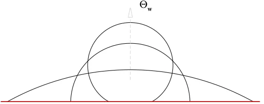
No-slip boundary condition is applied at the solid wall by using the halfway bounce-back scheme [60], where the wall is located halfway between the fluid node and solid node. Following our previous work [34, 61], the contact angle θis enforced at the wall through the geometrical formulation proposed by Ding and Spelt [41], i.e.,

~nw· ∇ρN =−Θw|~tw· ∇ρN| (22)

with

Θw= tan π

2 −θ

, (23)

where~nw is the unit normal vector to wall pointing towards the fluids, and~tw is the unit vector tangential to wall.

The enforcement of Eq. (22) is realized through the external solid nodes (also termed as ghost nodes), which are a half lattice spacing away from the wall. Without losing generality, we consider the case of bottom wall, whose neighboring solid and fluid nodes are located aty= 0 andy= 1, respectively. Upon discretization of Eq. (22), one has

ρNx,0=ρNx,1+ Θw|~tw· ∇ρN|δx, (24)

where the tangential component of∇ρN _{on the wall is determined by the following extrapolation scheme [59]:}

~tw· ∇ρN = 1.5∂xρN

x,1−0.5∂xρ N

x,2. (25)

In Eq. (25), the derivatives on the right-hand side can be easily evaluated by the second-order central difference approximation. Once the value of the phase fieldρN

C. Contact angle hysteresis model

The wetting boundary condition given in Subsect. II B is suited only for ideal (i.e., rigid, smooth, and chemically homogeneous) solid surfaces with a prescribed contact angle. However, most practical surfaces are rough and het-erogeneous to some extent, and the contact angle hysteresis can play a crucial role, e.g. the contact angle hysteresis allows a droplet to be held on a tilted plane and resists the gravity. The contact angle hysteresis is known as a phenomenon in which the contact line remains fixed at a given position, provided that the local contact angle θlies within the window of [36, 40, 62]

θR< θ < θA, (26)

where θA and θR denote the advancing and receding angles, respectively. On the other hand, if θ is beyond the

hysteresis window, the contact line will move with the moving direction depending on the relative magnitude of θ, θA and θR. Specifically, ifθ ≥θA, the contact line moves forward; if θ ≤θR, the contact line moves backward. To

realize the effect of hysteresis, serval numerical strategies have been developed based on the macroscopic multiphase approaches and LBMs [34, 36, 40, 59, 63, 64]. In the present color-fluid LBM, we follow the strategy originally proposed by Ding and Spelt [40] due to its ease in implementation, which can be described as follows. At each time step of simulation, we first keep the values ofρN

x,0unchanged for all solid nodes (taken from the last time step), and obtain an initial estimate of the local contact angle,θ0, by the use of Eqs. (22) and (23). Then,ρNx,0is determined by comparing θ0 withθA and θR: if θ0≥θA, then setθ=θA and updateρNx,0 through Eqs. (24) and (25); if θ0 ≤θR,

then setθ=θR and updateρNx,0through Eqs. (24) and (25); otherwise, we let ρNx,0unchanged.

Note that we here implement the contact angle hysteresis with a given hysteresis window. Due to the microscopic origin of hysteresis, actually, the hysteresis window is determined by the properties of the solid surface in contact with the droplet such as surface roughness and nonuniformity [2, 65]. Microscopically, there have been a number of recent works revealing the importance of the contact angle hysteresis and dynamic contact angle [66–68], but the study of the contact angle hysteresis from a viewpoint of microscale is beyond the scope of this work.

III. RESULTS AND DISCUSSION

A. Droplet deposited on an ideal substrate with prescribed contact angles

First, we investigate the equilibrium shapes of a droplet on an ideal substrate to examine the model’s capability in simulating prescribed contact angles. Simulations are performed in a 240×160 lattice domain, and a semi-circular droplet (red fluid) with the radiusR= 32 is initially deposited on the bottom wall. The periodic boundary condition is used in thex-direction while the wetting boundary condition, which is given in Subsection II B, is imposed at the top and bottom walls in the y-direction. It is known that most existing multiphase/multicomponent LBMs would suffer from numerical instability when the binary fluids have large kinematic viscosity ratio [69]. For instance, the kinematic viscosity ratio is restricted to typically less than 6 in the most-used interparticle-potential LBM [70]. To check whether this also happens to the present model, two different kinematic viscosity ratios (M = νR/νB) are

investigated: (a) M = 1 with νR = νB = 0.35, and (b) M = 100 with νR = 0.35 and νB = 0.0035. The other

parameters are fixed as ˜ρR= ˜ρB= 1 and σ= 0.02. The velocity and density fields are initialized as~u= 0 and

ρR= ˜ρR, ρB= 0 if (x−120)2+ (y−0.5)2≤R2;

ρR= 0, ρB= ˜ρB otherwise. (27)

Based on these velocity and density fields, one can determine the initial distribution functions by their equilibrium values, i.e. fi = fieq and fik = ρ

k

ρR+ρBf

eq

i for k = R or B. Each simulation is run until the shape of droplet

does not change, i.e., reaching an equilibrium state. Different contact angles can be achieved through adjusting the dimensionless parameter Θw according to Eq. (22). Fig. 1 shows equilibrium shapes of the droplet with Θw =

√

3, 0 and −√3 for the viscosity ratio M = 100. Their corresponding equilibrium contact angles, calculated from the measured droplet height and base diameter, are 29.68◦_{, 89.96}◦ _{and 152.68}◦_{, respectively. The simulated equilibrium} contact angle (θeq_{) as a function of Θ}

w forM = 1 andM = 100 is presented in Fig. 2. As expected, the simulations

are stable in the entire range of contact angles from 30◦ _{to 150}◦ _{for both M = 1 and M = 100. Also, it is clearly} observed that the simulation results are independent of the viscosity ratio, in good agreement with the theoretical solution, i.e., Eq. (23). A numerical artifact observed in many numerical methods is the presence of spurious velocities at the phase interface. This is also true in our case. Table I shows the maximum spurious velocities (|~u|max) at various

θeq _{forM = 1 and 100, where the values of|~u|}

Θ

FIG. 1: (Color online) Equilibrium droplet shapes obtained through adjusting the dimensionless parameter Θw forM = 100.

The values of Θw are taken as √

3, 0, and−√3 along the direction of arrow.

Θ

θ

eq

-2 -1 0 1 2

0 30 60 90 120 150 180

LBM (M=1) LBM (M=100) Theory

FIG. 2: Contact angle as a function of Θw for the viscosity ratiosM = 1 (represented by triangles) and 100 (represented by

circles). The solid line represents the theoretical predictions by Eq. (23).

atM = 1, the maximum spurious velocities are on the order of 10−4 _{or even smaller, comparable to those produced} by the color-fluid model that used the wetting boundary condition of Ba et al. [61]. It is also seen in Table I that the maximum spurious velocities increase with the viscosity ratio, but most of them are still on the order of 10−4 _{for the} viscosity ratio as high as 100.

B. Capillary intrusion

TABLE I: The maximum spurious velocities (|~u|max) at variousθeq for M= 1 and 100. All angles are shown in degrees.

θeq _{30 45 60 90 120 135 150}

|~u|max×10

4 M = 1 0.900 0.340 0.192 0.043 0.582 1.301 2.160 M= 102

19.49 6.981 8.981 0.119 8.943 8.406 11.85

L

wetting fluid

r

non-wetting fluid

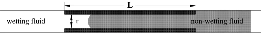
FIG. 3: Simulation setup for capillary intrusion. The portion in the center of the domain is a capillary tube of lengthL and widthr. The intruding fluid is wetting with respect to the tube while the defending fluid is non-wetting.

a wetting fluid column intruding a horizontal capillary tube with ideal surfaces, as shown in Fig. 3, is determined by the balance between the pressure difference over the interface, the Laplace pressure, and the viscous drag of the intruding fluid. If the gravity and inertial effects are neglected, this balance can be expressed as [72, 73]

σcos(θ) =6

r[µRξ+µB(L−ξ)] dξ

dt, (28)

whereθis the contact angle,ris the width of capillary tube ,ξis the position of the moving interface withξ= 0 at the inlet of capillary tube, andµRandµB are the dynamic viscosities of the red (wetting) and blue (non-wetting) fluids,

respectively. In the analytical derivation,θ is specified as a wall boundary condition. However, for comparison with simulations or experiments,θis better taken as the dynamic contact angle [72, 73]. The system consists of a 400×35 lattice domain with periodic boundary conditions used in thex-direction. In the middle portion, i.e. 100≤x≤300, the boundaries of the capillary tube are no-slip and wetting with Eq. (22) imposed on them. The length of the capillary tube is taken as L = 200 lattices. Outside of the middle portion, the boundary conditions are periodic in the y-direction, mimicking an “infinite reservoir”. The simulations are run with the parameters ˜ρR = ˜ρB = 1,

σ= 5×10−3_{andr= 21 for two different viscosity ratios: (a)M = 1 and (b)M = 100. The dimensionless parameter} Θwis chosen as 1.0 to represent hydrophilic capillary tube for the intruding red fluid. In the fluid domain, the blue

fluid is initialized at the position 120 ≤ x ≤ 375, and the remaining lattice sites are filled with red fluid. fi, fiR

and fB

i are then initialized using the zero velocity equilibrium distribution functions. Fig. 4 shows the comparison

between our simulation results and the analytical predictions from Eq. (28) forM = 1 and 100. Note that Eq. (28) is plotted using the dynamic contact angle, measured from our simulations. ForM = 1 andM = 100, the measured dynamic contact angles are respectivelyθ = 46.84◦ _{and 47.11}◦_{, which are very close but slightly deviate from their} prescribed value 45◦_{. It can be seen that the present color-fluid LBM can predict Eq. (28) pretty well for a broad} range of viscosity ratios.

C. Droplet on a non-ideal substrate subject to a shear flow

A droplet attached on a nonideal substrate subject to a shear flow is investigated to test the hysteresis behavior of contact angle. We first simulate a droplet pinned on the solid surface due to a large hysteresis window, and the obtained results are compared with the previous numerical results. Then we investigate the influence of hysteresis window and viscosity ratio on droplet behavior at a fixed capillary number.

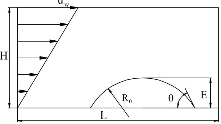
First, we follow the previous studies [36, 59, 64] and consider the deformation of a droplet on a non-ideal wall with contact angle hysteresis in a shear flow. This test aims to verify if the contact angle hysteresis is correctly incorporated in our color-fluid LBM. As shown in Fig. 5, the two walls are separated by a distanceH. The bottom wall is kept stationary, and the top wall moves towards the right with a constant velocityuw. Periodic boundary conditions are

applied in the horizontal direction. Both fluids have the same density and viscosity, which are given by ˜ρR = ˜ρB =

1, and νR =νB = 0.2, respectively. The interfacial tension is set to beσ= 5×10−3. Initially, a droplet of circular

segment (red fluid) with the radius R0 and contact angleθ = 60◦ is deposited on the bottom wall. Note that one needs to initially specify the phase field of the ghost nodes, i.e. ρN

x,0, when the contact angle hysteresis is considered. ρN

t

ξ

(t

)

0 2 4 6

0 50 100 150 200

(b) M=100

×105

t

ξ

(t

)

0 2 4 6 8 10

0 50 100 150 200

(a) M=1

×105

FIG. 4: (Color online) The length of the column of the intruding fluid,ξ(t), versus time for the viscosity ratios of (a)M = 1 and (b)M= 100. The (red) open circles represent the simulation results of LBM and the (blue) solid lines are the theoretical predictions from Eq. (28).

FIG. 5: Schematic diagram of a droplet meniscus on a non-ideal substrate subject to a simple shear flow.

with stationary walls (by setting uw = 0 as well) and the constant contact angle of 60◦ until reaching the steady

state, and then assign the steady-state phase field as the initial phase field of the hysteresis simulation. According to the initial phase field ρN_{(~x), the initial values of the fluid densities are determined by ρ}

R(~x) = 1+ρ

N

(~x)

2 and

ρB(~x) = 1−ρ

N

(~x)

2 , and the distribution functions fi, fiR and fiB can be initialized using their corresponding zero

velocity equilibrium distributions. The problem is characterized by two important parameters: the scaled droplet area, defined byA∗

d= 4Ad/H2 withAd being the droplet area, and the capillary numberCa=µBuwE/(σH), where

Eis the initial height of the droplet. We perform the simulations in aL×H= 500×250 lattice domain forCa= 0.05, 0.1, and 0.15 at a constantA∗_d = 0.5. A large hysteresis window (θR, θA) = (5◦,175◦) [59] is imposed through the

strategy given in Subsection II C so that the droplet remains pinned on the bottom wall. This allows us to compare our results with those obtained by Schleizer and Bonnecaze [74], where a boundary element method was used.

Fig. 6 compares the simulated equilibrium droplet shapes with the numerical results of Schleizer and Bonnecaze [74] forCa= 0.05, 0.1, and 0.15 atA∗

d= 0.5. As Caincreases, the droplet deforms more significantly, and the difference

between the downstream and upstream contact angles increases. For all of the capillary numbers, the simulated droplet shapes (represented by solid lines) agree well with the results of Schleizer and Bonnecaze (represented by dashed lines), revealing good accuracy of the present model for handling contact angle hysteresis.

(x-x

)/R

(y

-y

0

)/

R

-1

-0.8

-0.6

-0.4

-0.2

0

0.2

0.4

0.6

0.8

1

-1

-0.9

-0.8

-0.7

-0.6

-0.5

(b)

(x-x

)/R

(y

-y

0

)/

R

-1

-0.8

-0.6

-0.4

-0.2

0

0.2

0.4

0.6

0.8

1

-1

-0.9

-0.8

-0.7

-0.6

-0.5

(a)

(x-x

)/R

(y

-y

)/

R

-1

-0.8

-0.6

-0.4

-0.2

0

0.2

0.4

0.6

0.8

1

-1

-0.9

-0.8

-0.7

-0.6

-0.5

(c)

FIG. 6: Comparison of the simulated equilibrium droplet shapes with the numerical results of Schleizer and Bonnecaze [74] for Ca= 0.05, 0.1, and 0.15 at A∗

d = 0.5. The solid lines are the present LBM simulation results, while the dashed lines are

the results of Schleizer and Bonnecaze. Thex- andy-coordinates relative to the center of computational domain (x0, y0) are

normalized byR0.

fixed capillary number and viscosity ratio. A semicircular droplet of radiusR0= 64 is initially placed on the bottom wall in a 1024×128 lattice domain. Both fluids are assumed to have equal density and kinematic viscosity, i.e., ˜

ρR = ˜ρB = 1 and νR =νB = 0.25, and the interfacial tension is set as σ = 10−3. We use the same initialization

strategy and boundary conditions described above (except that the initial contact angle θ = 90◦_{), and choose the} moving velocity of the top walluw= 2.56×10−3such thatCa= 0.32 andRe=uwR20/(HνB) = 0.328. Besides, the

hysteresis windows are chosen as (0◦_,180◦_{), (0}◦_,110◦_{), (70}◦_,180◦_{), and (70}◦_,110◦_{), which have been used recently by} Wang et al. [64] for qualitatively testing their model.

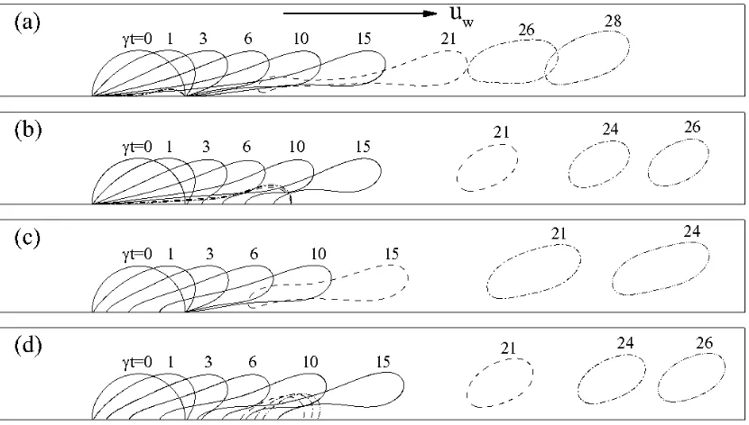
Fig. 7 shows the snapshots of droplet motion for the hysteresis windows of (0◦_,180◦_{), (0}◦_,110◦_{), (70}◦_,180◦_{), and} (70◦_,110◦_{) atM = 1 andCa= 0.32, where the dimensionless time is defined ast}∗_{=γtwith the shear rateγ=u}

w/H.

In the early stages, the droplet deforms and/or moves downstream on the bottom wall. As expected, one can observe four typical motion modes of the contact points (note that we use the contact point instead of the contact line in two-dimensional problems) due to four hysteresis windows. For (θR, θA) = (0◦,180◦), both the upstream and downstream

contact angles cannot go outside of the hysteresis window, so both contact points always remain motionless on the solid surface. For (θR, θA) = (0◦,110◦), due to strong shear stresses from the carrier fluid the upstream contact

FIG. 7: Snapshots of droplet motion for the hysteresis windows of (0◦_,180◦_{), (0}◦_,110◦_{), (70}◦_,180◦_{), and (70}◦_,110◦_{) atM = 1}

andCa= 0.32. Note that the droplet profiles are represented successively by the dashed lines, dash-dot lines and dash-dot-dot lines at the final three instants after the breakup or detachment from the wall.

angle is less than 110◦_{, and later it moves downstream as long as the contact angle becomes larger than 110}◦_{. For} (θR, θA) = (70◦,180◦), the downstream contact angle keeps increasing continuously, but it stays in the range of

hysteresis window at all times, resulting in the downstream contact point immobilized. For the upstream contact point, during the initial short time (typically when γt ≤1) it is pinned because the instantaneous contact angle is larger than 70◦_{, and later it progresses downstream along the surface when the contact angle is less than 70}◦_{. For} (θR, θA) = (70◦,110◦), the droplet keeps pinned and deforms continuously until the upstream and downstream contact

angles reach their hysteresis limits, and then starts to slip over the wall. These results are in qualitative agreement with the previous computations of Wang et al. [64], which is built upon the mean-field theory model. As the droplet deforms and/or the contact points (which might be the upstream contact point only, the downstream contact point only, or both) progress downstream further, one can observe two different dynamical behaviors of droplet in the late stages. Specifically, if (θR, θA) = (70◦,180◦), the droplet departs entirely from the solid surface and finally moves

at a constant velocity in the carrier fluid free of wetting effects; otherwise, the droplet breaks up into two separate parts: one moves fast as it breaks away from the solid surface, while the other adheres to the solid surface with its shape, size and motion state depending on the hysteresis window. Clearly, the adhering part eventually remains immobilized for (θR, θA) = (0◦,180◦) and (0◦,110◦), but slides over the surface at a constant, relatively low velocity

for (θR, θA) = (70◦,110◦).

In addition, we also simulate the deformation, breakup and migration of the droplet at various hysteresis windows for the viscosity ratio of 0.01, and the obtained results will be compared with the case ofM = 1 (see Fig. 7) to show the influence of viscosity ratio on the hysteresis behavior. All the simulation parameters are kept the same as in the case of M = 1 except that the viscosity of the dispersed phase (red fluid) is changed to beνR= 0.0025. Fig. 8

illustrates the time evolution of droplet shapes for the hysteresis windows of (0◦_,180◦_{), (0}◦_,110◦_{), (70}◦_,180◦_{), and} (70◦_,110◦_{) atM = 0.01 andCa= 0.32. For (θ}

R, θA) = (0◦,180◦), both the upstream and downstream contact points

remains pinned on the bottom wall at all times. From its initial semi-circular shape, the droplet gradually deforms and finally reaches a stationary shape (represented by the red bold lines in Fig. 8(a)). In contrast, for M = 1 the droplet continuously deforms and eventually breaks up into two parts, one of which remains pinned on the bottom wall forever and the other moves downstream in the carrier fluid (see Fig. 7(a)). For (θR, θA) = (0◦,110◦), the

FIG. 8: (Color Online) Snapshots of droplet motion for the hysteresis windows of (0◦_,180◦_{), (0}◦_,110◦_{), (70}◦_,180◦_{), and}

(70◦_,110◦_{) atM = 0.01 andCa= 0.32. In (a) and (b), the droplet profiles in the steady state are represented by the (red)}

bold lines, while in (c) the droplet profiles are represented successively by the dashed lines, dash-dot lines and dash-dot-dot lines at the final three instants after the detachment from the wall.

FIG. 9: (Color Online) Snapshots of droplet motion in the coarse and fine grids for the hysteresis windows of (a) (0◦_,110◦_{) and}

(b) (70◦_,110◦_{) atM = 0.01 andCa= 0.32. Note that the droplet profiles in the coarse and fine grids are shown by the black}

solid lines and the red dashed lines, respectively. Thex- andy-coordinates relative to the center of computational domain (x0, y0) are normalized byR0.

small ones, as illustrated in Fig. 7(b). For (θR, θA) = (70◦,180◦), the droplet motion (including the motion of both

contact points) exhibits similar behavior to those observed in the case ofM = 1; nevertheless, there exists quantitative difference in the droplet shape and terminal velocity, as well as the velocity of moving contact point for bothM = 0.01 andM = 1. For (θR, θA) = (70◦,110◦), in the early stages the motion of contact points is analogous to the previous

observation ofM = 1; whereas in the late stages the droplet reaches a steady shape and slides over the bottom wall at a constant velocity, differing significantly from the pinch-off behavior observed in the case ofM = 1. Thus, it can be concluded that the viscosity ratio plays an extremely important role in determining the dynamical behavior of a droplet when the contact angle hysteresis is taken into account.

(x-x

)/R

(y

-y

)/

R

-6 -5 -4 -3

-1 -0.5 0 0.5

(a)

(x-x

)/R

(y

-y

0

)/

R

2 3 4 5

-1 -0.5 0 0.5

(b)

FIG. 10: (Color online) The velocity vectors and streamlines around the droplet for (a) (θR, θA) = (0◦,110◦) in the steady

state and (b) (θR, θA) = (70◦,110◦) atγt= 34 in the computational domain of 1024×128 grids. Note that the droplet profiles

are represented by the red dashed lines, and thex- andy-coordinates relative to the center of computational domain (x0, y0)

are normalized byR0.

simulated: one with the hysteresis window of (0◦_,110◦_{), and the other with (70}◦_,110◦_{). Both cases have the same} viscosity ratio, capillary number and Reynolds number, i.e., M = 0.01, Ca = 0.32 and Re = 0.328. Fig. 9 gives the comparison of simulation results between the coarse grid and the fine grid for (a) (θR, θA) = (0◦,110◦) and (b)

(θR, θA) = (70◦,110◦). Note in Fig. 9 that the simulation results in the coarse grid have been plotted previously in

Fig. 8(b) and (d). It is clearly seen that the grid refinement only has a slight effect on the simulation results, indicating that the coarse grid with the domain size of 1024×128 grids can provide acceptable numerical accuracy. Since the interface thickness decreases with the grid refinement, the slight effect of the grid refinement on the simulation results also indicates that a further decrease in the interface thickness almost has no effect on the simulation results, i.e. approaching the sharp-interface limit. Fig. 10(a) and (b) depict the velocity vectors and streamlines around the droplet interface in the coarse grid for (θR, θA) = (0◦,110◦) in the steady state and for (θR, θA) = (70◦,110◦) atγt= 34. For

(θR, θA) = (0◦,110◦), we can observe that two unequal-sized vortices are fully filled with the droplet inside, implying

that there is not momentum exchange between the droplet and the carrier fluid; whereas for (θR, θA) = (70◦,110◦),

FIG. 11: (Color Online) Schematic of T-junction geometry.

the droplet and the carrier fluid. These behaviors of streamlines are consistent with the motion of droplet over the solid surface. Also, we do not see unexpected vortices or weird variations of velocity in the vicinity of interface, in particular around the contact points, indicating that unphysical spurious velocities are effectively suppressed in the present LBM even when the contact angle hysteresis is considered.

D. Droplet breakup process at a microfluidic T-junction

As stated above, the color-fluid model proposed by Ba et al. [34] suffers from the difficulty of handling contact line dynamics with complex solid boundaries. In order to demonstrate that such a difficulty can be greatly overcome in the present model, we use it to simulate the droplet breakup process at a microfluidic T-junction, where the convex corner is also encountered in addition to the straight walls. We consider a red droplet of initial lengthL0= 120 that flows from a channel of widthwf = 40 and lengthlf = 200 into a T-junction with two equal arms of the same width

wa= 40 and lengthla= 400 (see Fig. 11). The droplet is carried downstream by the blue fluid, which flows through

the feed branch of the T-junction with the mean velocityU. The channel walls in the right half of the geometry are ideal with constant contact angle of 135◦_{, while the rest of channel walls are non-ideal with the hysteresis window of} (120◦_,150◦_{). For the sake of simplicity, both fluids are assumed to have equal densities, i.e. ˜ρ}

R = ˜ρB = 1, and the

interfacial tension is fixed at 0.02. Considering that the flow in the microchannel is typically laminar, the Reynolds number (Re = ˜ρBU wf/µB) is selected as 0.4 without loss of generality. The capillary number, which describes

the relative importance of viscosity to the interfacial tension and is defined by Ca=U µB/σ, is commonly used to

characterize the droplet breakup process, and its value is 5×10−3_{. In this subsection, we will examine whether} and how the contact angle hysteresis and the viscosity ratio influence the dynamics of droplet breakup. A parabolic velocity profile and a constant pressure are specified respectively, at the inlet and outlets using the non-equilibrium bounce-back scheme [75]. The no-slip boundary condition is applied at the wall surfaces. For the straight walls, the surface wettability is introduced directly following the method described in Sects. II B and II C; whereas for the convex corners, the following method is adopted to determineρN_{(x, y), where (x, y) represents the solid node most}

adjacent to the convex corner:

1. Suppose that (x, y) is the ghost node of the horizontal wall, and use the method described in Sects. II B and II C to determine the phase field at this node, denoted byρN

h;

2. Suppose that (x, y) is the ghost node of the vertical wall, and use the method described in Sects. II B and II C to determine the phase field at this node, denoted byρN

v;

3. UpdateρN_{(x, y) using the average of ρ}N

h andρNv , i.e. ρN(x, y) = ρNh +ρNv

/2.

We run the simulations at three different viscosity ratios, i.e. M = 3, 1 and 0.1, which are achieved by varying solely the viscosity of the red fluid. Each simulation is initialized with the density field

ρR= ˜ρR, ρB = 0 if 70≤y≤190;

FIG. 12: (Color Online) Snapshots of droplet breakup in the ‘non-ideal’ T-junction forCa= 5×10−3

andRe= 0.4 at different viscosity ratios: (a)M = 3, (b)M= 1 and (c)M = 0.1. For the T-junction, the right half walls are assumed to be ideal with the constant contact angle of 135◦_{, while the remaining walls are non-ideal with the hysteresis window of (120}◦_,150◦_{). The}

dimensionless time is defined byt∗_{=U t/w}

f. Note that the droplet and carrier fluid are shown in red and blue, respectively.

and zero velocity field everywhere except at the inlet, where the parabolic velocity profile is prescribed. By means of the density and velocity fields, the initial distribution functions are calculated asfi=fieq andfik =

ρk

ρR+ρBf

eq

i (k=R

orB).

Fig. 12 shows the snapshots of droplet breakup in the T-junction at three different viscosity ratios: (a) M = 3, (b) M = 1 and (c) M = 0.1. Note in Fig. 12 that the dimensionless time is defined by t∗ _{=U t/w}

f. The droplet

first moves downward and its head touches the bottom wall of the horizontal channel at around t∗ _{= 2. Later, the} droplet continues to fill the junction until completely entering the junction att∗_{= 3.5. During this time, the droplet} invades the left and right branches and advances inside, but the droplet advances more slowly in the left branch due to the contact angle hysteresis. Soon after t∗ _{= 3.5, a bent neck is formed under the squeezing of the carrier fluid} flowing into the T-junction. The span of the bent neck is gradually expanded, and the expansion mainly occurs in the right branch of the horizontal channel. This suggests that the carrier fluid mostly flows into the right branch as a result of the interface retardation in the left branch. The droplet eventually pinches off at its minimum width and is asymmetrically split into two daughter droplets. It is clearly seen that the daughter droplet in the branch with non-ideal surfaces is smaller than the other one. We interestingly note that, during the entire breakup process the droplet tips always keep touching with the channel walls, evincing that the horizontal channels are continuously obstructed by droplets. This is known as breakup with permanent obstruction (POB), which has been observed both experimentally and numerically in microfluidic T-junctions [76–78].

FIG. 13: (Color Online) Snapshots of droplet breakup in the ‘ideal’ T-junction with the contact angle of 135◦ _{for M = 1,} Ca= 5×10−3

and Re= 0.4. The snapshots are taken at the times: (a)t∗_{= 0, (b)t}∗ _{= 2, (c)t}∗ _{= 3.5, (d) t}∗_{= 4.5, (e)} t∗_{= 8.25, (f)t}∗_{= 8.375, (g)t}∗_{= 9, (h)t}∗_{= 13. Note that the droplet and carrier fluid are shown in red and blue, respectively.}

M = 3, the daughter droplet keeps migrating through the left branch channel, but at a velocity much lower than the right one (see t∗ _{= 10.25, 11.75 and 13 in Fig. 12(a); at medium and low viscosity ratios, i.e. M = 1 and 0.1, the} daughter droplet gets pinned in the left branch, but its rest position depends onM: the droplet remains ultimately pinned at a certain distance from the T-junction and at the junction corner for M = 1 and M = 0.1, respectively. These quantitative differences in the droplet behavior indicate that the contact angle hysteresis can be strengthened with the decrease ofM, consistent with the finding in Subsect. III C. In addition, we also quantify the length of the daughter droplet (Lr) in the right branch channel and find that the values ofLrare 73.2, 74.6 and 70.7 forM = 3, 1

and 0.1, respectively. Obviously,Lr varies non-monotonously with the decrease of viscosity ratio, but the variations

are not so noticeable in the cases under consideration.

Finally, we simulate the droplet breakup process at the T-junction with all the parameters unchanged except for the hysteresis window which is now (135◦_,135◦_{). Such a hysteresis window implies that the entire channel walls are} ideal with a constant contact angle of 135◦_{. Fig. 13 depicts the snapshots of droplet breakup in the T-junction for} (θR, θA) = (135◦,135◦) at M = 1. Compared to the case of (θR, θA) = (120◦,150◦) (see Fig. 12(b)), the droplet

pinches off at an earlier time, i.e. t∗ _{= 8.375, and the maximum length that the droplet can reach before the} pinch-off is smaller: specifically, the values of the maximum length are 306 and 337 for (θR, θA) = (135◦,135◦) and

(120◦_,150◦_{), respectively. Due to the symmetry of the channel geometry and the imposed surface wettability, the} droplet symmetrically moves and deforms, eventually breaking up into two equal-sized daughter droplets. The two daughter droplets then move at the same speed towards the outlets. These droplet behaviors are evidently different from the previous observations in the case of (θR, θA) = (120◦,150◦), suggesting that the hysteresis window is one of

important factors characterizing the droplet breakup process.

IV. CONCLUSIONS

contact angle is enforced through the geometrical formulation proposed in Ref. [41], with implementation following Huang et al. [59]. The color-fluid LBM is first validated by simulations of static contact angle and dynamic capillary intrusion on the ideal surfaces for the viscosity ratios of 1 and 100. It is then used to simulate the dynamic behavior of a droplet on a non-ideal surface subject to a shear flow. For the droplet pinned on the solid surface due to a large hysteresis window of contact angles, the predicted shapes of deformed droplet are in good agreement with the previous numerical results of Schleizer and Bonnecaze [74]. In the early stages (e.g. γt < 6), four typical motion modes of contact points, which were observed by Wang et al. [64], are qualitatively reproduced by adjusting the hysteresis windows. In addition, it is found that the viscosity ratio can affect not only the deformation and slipping velocity of the droplet but also its breakup and hysteresis behavior. To show the model’s capability in dealing with complex boundaries, we simulate the droplet breakup process in a microfluidic T-junction, where one half of the channel surface is ideal and the other half is non-ideal. For all of the viscosity ratios, the droplet finally breaks up into two unequal-sized daughter droplets with the smaller one in the non-ideal branch. However, decreasing the viscosity ratio can strengthen the effect of contact angle hysteresis, thereby leading to an earlier breakup of the droplet and a decrease in the maximum length that the droplet can reach before the breakup. Also, the daughter droplet in the ideal branch always keeps moving towards the outlet, but the daughter droplet in the non-ideal branch either moves at an extremely low velocity or remains pinned at a position, which strongly depends on the value of viscosity ratio. In summary, our numerical results indicate that the present color-fluid LBM is numerically stable and accurate for simulating binary fluids with a wide range of viscosity ratios, no matter whether the contact angle hysteresis is considered, and also can be easily extended for handling complex geometry.

Acknowledgments

This work is financially supported by the Thousand Youth Talents Program for Distinguished Young Scholars and the National Natural Science Foundation of China (No. 51406148).

[1] J. H. Snoeijer and B. Andreotti, Annu. Rev. Fluid Mech.45, 269 (2013). [2] P. G. de Gennes, Rev. Mod. Phys.57, 827 (1985).

[3] R. G. Cox, J. Fluid Mech.168, 169 (1986). [4] R. L. Hoffman, J. Coll. Interf. Sci.50, 228 (1975).

[5] T.-S. Jiang, O. Soo-Gun, and J. C. Slattery, J. Coll. Interf. Sci.69, 74 (1979).

[6] A. Jabbarzadeh and R. I. Tanner,Rheology Reviews (2006), chap. Molecular dynamics simulation and its application in nano-rheology, pp. 165–216.

[7] B. Shi and V. K. Dhir, THE JOURNAL OF CHEMICAL PHYSICS130, 034705 (2009). [8] E. Bertrand, T. D. Blake, and J. D. Coninck, J. Phys.: Condens. Matter21, 464124 (2009). [9] F.-C. Wang and Y.-P. Zhao, Colloid Polym. Sci.291, 307 (2013).

[10] C. Hirt and B. Nichols, J. Comput. Phys.39, 201 (1981).

[11] D. Gueyffier, J. Li, A. Nadim, R. Scardovelli, and S. Zaleski, J. Comput. Phys.152, 423 (1999), ISSN 0021-9991. [12] M. Sussman, E. Fatemi, P. Smereka, and S. Osher, Comput. Fluids27, 663 (1998).

[13] S. Osher and R. P. Fedkiw,Level sets methods and dynamic implicit surfaces (Springer, 2003). [14] L. M. Hocking, J. Fluid Mech.79, 209 (1977).

[15] H.-Y. Chen, D. Jasnow, and J. Vi˜nals, Phys. Rev. Lett.85, 1686 (2000). [16] J. Zhang, Microfluid. Nanofluid.10, 1 (2011).

[17] C. K. Aidun and J. R. Clausen, Annu. Rev. Fluid Mech.42, 439 (2010), ISSN 0066-4189. [18] S. Chen and G. D. Doolen, Annu. Rev. Fluid Mech.30, 329 (1998).

[19] A. K. Gunstensen, D. H. Rothman, S. Zaleski, and G. Zanetti, Phys. Rev. A43, 4320 (1991). [20] I. Halliday, R. Law, C. M. Care, and A. Hollis, Phys. Rev. E73, 056708 (pages 11) (2006). [21] T. Reis and T. N. Phillips, J. Phys. A-Math. Theor.40, 4033 (2007).

[22] H. Liu, A. J. Valocchi, and Q. Kang, Phys. Rev. E85, 046309 (2012).

[23] M. R. Swift, E. Orlandini, W. R. Osborn, and J. M. Yeomans, Phys. Rev. E54, 5041 (1996). [24] H. Zheng, C. Shu, and Y. Chew, J. Comput. Phys.218, 353 (2006).

[25] T. Lee and L. Liu, J. Comput. Phys.229, 8045 (2010). [26] X. Shan and H. Chen, Phys. Rev. E47, 1815 (1993). [27] X. Shan and H. Chen, Phys. Rev. E49, 2941 (1994).

[28] M. Sbragaglia, R. Benzi, L. Biferale, S. Succi, K. Sugiyama, and F. Toschi, Phys. Rev. E75, 026702 (2007). [29] X. He, S. Chen, and R. Zhang, J. Comput. Phys.152, 642 (1999).

[31] H. Liu and Y. Zhang, Phys. Fluids23, 082101 (2011).

[32] A. Gupta and R. Kumar, Microfluidics and Nanofluidics8, 799 (2010).

[33] H. Liu, A. J. Valocchi, C. Werth, Q. Kang, and M. Oostrom, Adv. Water Resour.73, 144 (2014). [34] Y. Ba, H. Liu, J. Sun, and R. Zheng, Phys. Rev. E 8888, 043306 (2013).

[35] A. P. Hollis, T. J. Spencer, I. Halliday, and C. M. Care, IMA J. Appl. Math.76, 726 (2011). [36] J.-B. Dupont and D. Legendre, J. Comput. Phys.229, 2453 (2010).

[37] C. M. Pooley, H. Kusumaatmaja, and J. M. Yeomans, Phys. Rev. E78, 056709 (2008).

[38] M. L. Porter, E. T. Coon, Q. Kang, J. D. Moulton, and J. W. Carey, Phys. Rev. E86, 036701 (2012). [39] H. Liu, A. J. Valocchia, Y. Zhang, and Q. Kang, J. Comput. Phys.256, 334 (2014).

[40] H. DING and P. D. M. SPELT, J. Fluid Mech.599, 341 (2008). [41] H. Ding and P. D. M. Spelt, Phys. Rev. E75, 046708 (2007).

[42] S. V. Lishchuk, C. M. Care, and I. Halliday, Phys. Rev. E67, 036701 (2003). [43] I. Halliday, A. P. Hollis, and C. M. Care, Phys. Rev. E76, 026708 (2007). [44] H. Liu, Y. Zhang, and A. J. Valocchi, J. Comput. Phys.231, 4433 (2012). [45] P. Lallemand and L.-S. Luo, Phys. Rev. E61, 6546 (2000).

[46] D. d’Humi`eres, I. Ginzburg, M. Krafczyk, P. Lallemand, and L.-S. Luo, Philos. Trans. R. Soc. A360, 437 (2002). [47] Y. H. Qian, D. D’Humi`eres, and P. Lallemand, Europhys. Lett.17, 479 (1992).

[48] Z. Yu and L.-S. Fan, Phys. Rev. E82, 046708 (2010).

[49] J. U. Brackbill, D. B. Kothe, and C. Zemach, J. Comput. Phys.100, 335 (1992), ISSN 0021-9991. [50] A. J. C. Ladd and R. Verberg, J. Stat. Phys.104, 1191 (2001).

[51] Z. Guo, C. Zheng, and B. Shi, Phys. Rev. E65, 046308 (2002). [52] Z. Chai and T. S. Zhao, Phys. Rev. E86, 016705 (2012).

[53] L.-S. Luo, W. Liao, X. Chen, Y. Peng, and W. Zhang, Phys. Rev. E83, 056710 (2011). [54] M. E. McCracken and J. Abraham, Phys. Rev. E71, 036701 (2005).

[55] Y. Q. Zu and S. He, Phys. Rev. E87, 043301 (2013).

[56] I. Ginzbourg and P. Adler, Transp. Porous Med.20, 37 (1995).

[57] A. Coward, Y. Renardy, M. Renardy, and J. Richards, J. Comput. Phys.132, 346 (1997). [58] M. Latva-Kokko and D. H. Rothman, Phys. Rev. E71, 056702 (2005).

[59] J.-J. Huang, H. Huang, and X. Wang, Phys. Fluids26, 062101 (2014). [60] A. J. C. Ladd, J. Fluid Mech.271, 285 (1994).

[61] H. Liu and Y. Zhang, J. Comput. Phys.280, 37 (2015). [62] P. Dimitrakopoulos and J. Higdon, J. Fluid Mech.395(1999). [63] P. D. Spelt, J. Comput. Phys.207, 389 (2005).

[64] L. Wang, H. bo Huang, and X.-Y. Lu, Phys. Rev. E87, 013301 (2013). [65] R. Tadmor, Langmuir20, 7659 (2004).

[66] N. Moradi, F. Varnik, and I. Steinbach, EPL (Europhysics Letters)89, 26006 (2010). [67] N. Moradi, F. Varnik, and I. Steinbach, EPL (Europhysics Letters)95, 44003 (2011).

[68] F. Varnik, M. Gross, N. Moradi, G. Zikos, P. Uhlmann, P. M¨uller-Buschbaum, D. Magerl, D. Raabe, I. Steinbach, and M. Stamm, J. Phys.: Condens. Matter23, 184112 (2011).

[69] H. Liu, Q. Kang, C. R. Leonardi, B. D. Jones, S. Schmieschek, A. Narvaez, J. R. Williams, A. J. Valocchi, and J. Harting, arXiv preprint arXiv:1404.7523 (2014).

[70] B. Dong, Y. Y. Yan, and W. Z. Li, Transp. Porous Med.88, 293 (2011). [71] E. W. Washburn, Phys. Rev.17, 273 (1921).

[72] F. Diotallevi, L. Biferale, S. Chibbaro, A. Lamura, G. Pontrelli, M. Sbragaglia, S. Succi, and F. Toschi, Eur. Phys. J. Special Topics166, 111 (2009).

[73] C. Pooley, H. Kusumaatmaja, and J. Yeomans, Eur. Phys. J. Special Topics171, 63 (2009). [74] A. D. Schleizer and R. T. Bonnecaze, J. Fluid Mech.383, 29 (1999).

[75] Q. Zou and X. He, Phys. Fluids9, 1591 (1997).

[76] M.-C. Jullien, M.-J. T. M. Ching, C. Cohen, L. Menetrier, and P. Tabeling, Phys. Fluids21, 072001 (2009). [77] A. M. Leshansky, S. Afkhami, M.-C. Jullien, and P. Tabeling, Phys. Rev. Lett.108, 264502 (2012).