Projected Powell-Sabin Splines
Oleg Davydov1⋆ and Larry L. Schumaker2
1
Department of Mathematics, University of Strathclyde, 26 Richmond Street, Glasgow G1 1XH, Scotland
2
Department of Mathematics, Vanderbilt University, Nashville, TN 37240
Abstract. We presentC1
methods for either interpolating data or for fitting scattered data associated with a smooth function on a two-dimen-sional smooth manifoldΩembedded intoR3
. The methods are based on a local bivariate Powell-Sabin interpolation scheme, and make use of local projections on the tangent planes. The data fitting method is a two-stage method. We illustrate the performance of the algorithms with some numerical examples, which, in particular, confirm theO(h3) order of convergence as the data becomes dense.
1
Introduction
LetΩbe a 2-dimensional smooth manifold. For simplicity we assume that Ωis compact and has no boundary. Suppose we are given the values of a (possibly unknown) smooth function f defined onΩ at a set of pointsX onΩ. Our aim is to construct a function s defined on Ω that approximates f. This problem arises frequently in practice, see Remark 1, but there do not seem to be many methods available for general manifolds. Several methods have been developed for the case whenΩ is the sphere, see Remark 2.
Our approach to solving this problem is as follows. Suppose we have an atlas
Φ={(Uξ, φξ)}ξ∈Ω forΩ, where for eachξ∈Ω,Uξare open sets onΩcontaining
ξ, andφξ are mappings ofUξ intoR2. We assume that theφξ depend smoothly onξin a certain sense, see [7]. Then for eachξ∈Ω, we project the data locations into φξ(Uξ)⊂R2, and use a local bivariate Powell-Sabin spline to compute the values(ξ) of the approximating functions. The resulting functionsisC1onΩ, and it has the usual approximation properties of the Powell-Sabin spline. This approach is related to methods for interpolation and data fitting on manifolds introduced by Demjanovich [10, 11] and Pottmann [25], see Remarks 3 and 4.
In this paper we examine the case when Ω is aC2-surface, i.e. a compact 2-dimensionalC2-manifold embedded inR3. Our implementation is based on a natural atlasΦdefined by local projections onto the tangent planes at all points on the surface Ω, see Section 2.1. General smooth 2-manifolds are treated in [7], where we also prove the main theoretical results about smoothness ofsand error bounds for interpolation and data fitting.
The paper is organized as follows. In Section 2 we introduce some basic con-cepts and notation. In Section 3 we first present a method for constructing an interpolant to the data on any smooth 2-dimensional manifold Ωembedded in R3, assuming we are also given values for the gradients at each of the data points inX. Next, we describe a two-stage data fitting method that works only with the data {fξ}ξ∈X, and which is more appropriate than interpolation for large data sets or noisy data. Theoretical results onC1 smoothness of the interpolating or approximating functions on Ω, as well as error bounds for the approximation of smooth functions are given here without proof. Numerical examples are pre-sented in Section 4 for both the sphere and for certain ring-type manifolds. We conclude the paper with remarks and references.
2
Preliminaries
2.1 Projection atlas
Leth·,·ibe the usual inner product inR3, and letkak2 be the Euclidean norm of any 3-vector a. Since Ω is embedded in R3, it can be represented locally as a regular level surface of a C2 function of three variables. More precisely, each point ξ ∈ Ω has a neighborhood Gξ in R3 such that Gξ∩Ω = Fξ−1(0), where Fξ : Gξ →R is a C2 function with nonzero gradient∇Fξ everywhere in
Gξ∩Ω, see [17]. Then nξ :=∇Fξ(ξ)/k∇Fξ(ξ)k2 is anormal vector toΩ at ξ. Moreover, thetangent plane Γξ is the unique plane inR3that containsξand is orthogonal tonξ. Clearly, for allζ∈ Gξ∩Ω, a normal vector toΩatζ can also be computed as∇Fξ(ζ)/k∇Fξ(ζ)k2. It coincides with either nζ or−nζ. Clearly,
hnξ,∇Fξ(ζ)i>0 for allζ∈ Gξ∩Ω.
We are now ready to define an atlas associated with Ω. For each ξ ∈ Ω, let Uξ be the connected component of the open set {ζ ∈ Ω : hnξ, nζi 6= 0} that contains ξ. Then Uξ is an open neighborhood ofξ. Clearly, theorthogonal
projection πξ:Uξ →Γξ defined by
πξ(ζ) =ζ+hξ−ζ, nξinξ, ζ∈Uξ,
is invertible. Assuming thatγ[1]ξ , γξ[2]are orthogonal unit vectors inΓξ such that
γξ[1]×γξ[2]=nξ, we can also write
πξ(ζ) =ξ+hζ−ξ, γ [1] ξ iγ
[1]
ξ +hζ−ξ, γ [2] ξ iγ
[2] ξ . Defineφξ by the formula
φξ(ζ) := [hζ−ξ, γ [1]
ξ i,hζ−ξ, γ [2] ξ i]
T, ζ
∈Uξ.
We callΦ={(Uξ, φξ)}ξ∈Ω theprojection atlas associated withΩ, and (Uξ, φξ),
ξ∈Ω, are itscharts.
Let us show thatΦis indeed an atlas in the sense of the standard definition of aC1-manifold, see e.g. [17]. This requires thatφ
betweenUξ and an open subset ofR2. Moreover, for everyξ, ζ∈Ω,φζξ:=φζ◦
φ−ξ1:φξ(Uζ∩Uξ)→φζ(Uζ∩Uξ) should be aC1mapping wheneverUξ∩Uζ 6=∅. Clearly, φξ is invertible by the choice of Uξ. Consider the coordinate sys-tem for R3 with coordinate vectorsγξ[1], γξ[2], nξ and origin ξ. For anyµ ∈ Uξ, the equation Fµ = 0 determines an implicit function x[3] = δµ(x[1], x[2]) in a neighborhood ofφξ(µ), such that
φ−ξ1(x[1], x[2]) =ξ+x[1]γξ[1]+x[2]γξ[2]+δµ(x[1], x[2])nξ.
Since hnξ,∇Fµ(µ)i = hnξ, nµik∇Fµ(µ)k2 6= 0, the implicit function theorem implies thatδµ(x[1], x[2]) is aC2function in a neighborhood ofφξ(µ). Assuming
µ∈Uξ∩Uζ, we also have
(φζ◦φ−ξ1)(x
[1], x[2]) =φ
ζξ(x[1], x[2]) = [φ [1] ζξ(x
[1], x[2]), φ[2] ζξ(x
[1], x[2])]T,
where fori= 1,2,
φ[i]ζξ(x[1], x[2]) =hξ−ζ+x[1]γξ[1]+x[2]γξ[2]+δµ(x[1], x[2])nξ, γζ[i]i (1)
in a neighborhood ofφξ(µ). Thereforeφζξ:φξ(Uξ∩Uζ)→φζ(Uξ∩Uζ) is aC2 mapping. Note that even if aC1 mappingφ
ζξwould suffice for our goals, we do need the assumption thatΩis aC2surface to ensure that the normalnξ changes smoothly withξ, which guarantees theC1smoothness of our approximants, see [7].
For aC1functionf defined in a neighborhoodU ofζ∈Ω, we defineJζ(f) :
U∩Uζ →R2×2 by
Jζ(f)(µ) :=J(f◦φζ−1)(φζ(µ)), µ∈U∩Uζ,
where for any smooth function g : R2 → R2, g = [g[1], g[2]]T, J(g) denotes its
Jacobian
J(g) :=
"∂g[1] ∂x[1]
∂g[1] ∂x[2] ∂g[2] ∂x[1]
∂g[2] ∂x[2]
#
.
We write
Jζξ:=Jξ(φζ), onUζ∩Uξ, so that
Jζξ(µ) =Jξ(φζ)(µ) =J(φζξ)(φξ(µ)), µ∈Uζ∩Uξ,
is the Jacobian of φζξ evaluated at φξ(µ). Since φ−ζξ1 = φξζ, the well-known properties of the Jacobian imply
[Jζξ(µ)]−1=Jξζ(µ). (2)
For later use, we now obtain explicit formulas for the JacobianJζξ(ξ) :=
above construction, the implicit functionx[3]=δ
ξ(x[1], x[2]) isC2 in a neighbor-hood of the originφξ(ξ). Moreover, it vanishes together with its gradient at the origin. Hence, by (1),
Jζξ(ξ) = [hγζ[i], γ [j]
ξ i]i,j=1,2. (3)
Clearly, the determinant of this matrix is the projection of nζ =γζ[1]×γ [2] ζ on
nξ, i.e.,
detJζξ(ξ) =hnζ, nξi. (4)
2.2 Projected gradients
Letf ∈C1(Ω), and let f
ξ =f ◦φ−ξ1. SinceΩis embedded inR3, the gradient
∇fξ =
h ∂f ξ
∂x[1], ∂fξ
∂x[2]
i
offξ can be identified with the 3-vector
gradfξ =
∂fξ
∂x[1]γ [1] ξ +
∂fξ
∂x[2]γ [2] ξ
lying in the tangent plane Γξ⊂R3. We write
gradξf(µ) := (gradfξ)(φξ(µ)), µ∈Uξ,
for the gradient offξevaluated atφξ(µ). We call gradξf(µ) theprojected gradient of f atµ. It is easy to see that gradξf(ξ) coincides with the standard gradient of a function on a 2-surface inR3, as defined for example in [28, p. 96]. We also need projected gradients when µ6=ξ.
Lemma 1. For anyξ∈Ω andζ∈Uξ, the projected gradientgradζf(ζ)is the
orthogonal projection ofgradξf(ζ)ontoΓζ. In particular,
gradζf(ζ) = gradξf(ζ)− hgradξf(ζ), nζinζ, (5)
and
gradξf(ζ) = gradζf(ζ)−
hgradζf(ζ), nξi
hnζ, nξi
nζ, if hnζ, nξi 6= 0, (6)
wherenζ andnξ are the unit normal vectors toΓζ andΓξ, respectively.
Proof.We have
gradξf(ζ) =
∂fξ
∂x[1]
φξ(ζ)
γξ[1]+ ∂fξ
∂x[2]
φξ(ζ)
γξ[2].
Its projection ontoΓζ is therefore
∂f
ξ
∂x[1]
φξ(ζ)
hγξ[1], γζ[1]i+ ∂fξ
∂x[2]
φξ(ζ)
hγξ[2], γζ[1]i
γζ[1]
+
∂f
ξ
∂x[1]
φξ(ζ)
hγξ[1], γζ[2]i+ ∂fξ
∂x[2]
φξ(ζ)
hγξ[2], γζ[2]i
This last expression coincides with gradζf(ζ), since
∇fζ(φζ(ζ)) =∇fξ(φξ(ζ))Jξζ(ζ) =∇ξf(ζ) [hγ [i] ξ , γ
[j] ζ i]i,j=1,2 by the chain rule and (3).
The formulas (5) and (6) for the projection and inverse projection, respec-tively, follow immediately.
2.3 Consistent triangulations
Given a finite set V of points in Ω, let T be a set of triples τ = {v, u, w} of pointsv, u, w∈ V such that
– any two triples have at most two common points,
– any pair of points inV belong to at most two different triples in T, and – for anyv ∈ V, the set of all triples containingv forms a cell, i.e. {τ ∈ T :
v ∈τ} ={τi : i= 1, . . . , n} for some n≥3, where τi ={v, vi, vi+1}, with
v1, . . . , vn all different, andvn+1=v1.
If these conditions are satisfied, we say that T is a triangulation of Ω with
vertices V. We say that two verticesv1, v2areconnected inT if there is a triple
τ ∈ T containing bothv1andv2. This definition of a triangulation of a manifold
Ω is described by connectivity of vertices only, and does not involve “edges” or “triangles” onΩ. Indeed,T is essentially anabstract simplicial complex [21] with vertices inΩ.
Givenξ∈Ω, assuming that all vertices ofτ={v, u, w} ∈ T are inUξ, we de-note byφξ(τ) the (open) planar triangle inBξ with verticesφξ(u), φξ(v), φξ(w). Note that the triangleφξ(τ) may be degenerate. We setTξ={τ∈ T : τ ⊂Uξ} and△ξ ={φξ(τ) : τ∈ Tξ}.
Definition 1. A triangulationT ofΩ is said to beconsistent with the projec-tion atlasΦ={(Uξ, φξ)}ξ∈Ω if for anyξ∈Ω,
– every triangleT ∈ △ξ is non-degenerate, – △ξ is a planar triangulation ofPξ:=∪T∈△ξT,
– φξ(ξ) lies in the interior ofPξ.
For anyξ∈Ω, letVξ be the set consisting of vertices of allτ∈ Tξ such that
φξ(ξ) lies in the closure ofφξ(τ), i.e.
Vξ:={v∈ V ∩Uξ :φξ(ξ)∈φξ(τ) for someτ∈ Tξ with a vertex atv}. For a consistent triangulationT, it is not difficult to check thatVζ ⊆ Vξ for all
In addition to consistency, we will need the following assumption, specifically related to the Powell-Sabin spline:
for everyξ∈Ω, ifφξ(ξ)∈Tfor aT ∈ △ξ, then△ξ also includes
three triangles sharing edges withT. (7)
We extend Vξ to ˜Vξ by adding to Vξ the vertices of the triangles described in (7).
3
Interpolation and data fitting
3.1 An interpolation method
LetT be a consistent triangulation ofΩ. We assume thatT is fine enough for (7) to hold. LetD:={av, cv}v∈V, whereavare real numbers andcv are 3-vectors in
Γv. We now show how to construct aC1 functionsT defined onΩthat satisfies
the interpolation conditions
sT(v) =av, gradvsT(v) =cv, allv∈ V. (8)
Algorithm 1. Given ξ∈Ω, computesT(ξ):
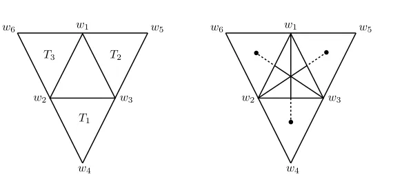
1. Let T := hw1, w2, w3i be a triangle in △ξ such that φξ(ξ) ∈ T, and let
T1 :=hw4, w3, w2i, T2 := hw5, w1, w3i, and T3 :=hw6, w2, w1i be the three
triangles in△ξ sharing edges withT, see Figure 1(left).
2. Let TP S be the Powell-Sabin split of T into six triangles obtained by
con-necting the incenterwofT to the incenters ofT1, T2, T3, and to the vertices
w1, w2, w3, see Figure 1(right).
3. Letgi :=cvi− hcvi,nξi
hnvi,nξinvi, wherevi=φ −1
ξ (wi), for i= 1,2,3.
4. Let sT(ξ) be the value at φξ(ξ) of the Powell-Sabin C1 quadratic spline sξ
defined onTP S that interpolates the values {avi}
3
i=1 and the gradients
cor-responding to{gi}3i=1 at the vertices {wi}3i=1, see[26].
Since the Powell-Sabin interpolant in step 4 is uniquely defined by the values
{(avi, gi)}
3
i=1 at the vertices{wi}3i=1, it follows that sT is uniquely defined by
the dataD. By construction,sT satisfies (8). It would be tempting to consider
sT to be a spline on a partition of the manifoldΩ obtained by drawing curves
onΩbetween connected vertices ofT. Indeed,sT possesses a kind of piecewise
structure, see [7]. However, this does not seem to be of a practical significance. What is important is thatsT is a smooth function.
Theorem 1 ([7]).The interpolantsT defined by Algorithm 1 is a C1 function
on the manifold Ω.
Suppose thatsT(f) is the interpolantsT corresponding to the data
w6 w1 w5
w2 w3
w4
T1
T2
T3
w6 w1 w5
w2 w3
w4
• •
[image:7.595.176.461.105.235.2]•
Fig. 1.The triangles in Algorithm 1.
where f is a smooth function defined on Ω. Denote by h the mesh size of T, by which we mean in the current setting the maximum distance inR3 between any pair of vertices v ∈ V connected in T. By actually connecting these pairs of vertices by straight line segments, we obtain a 2-dimensional triangulation in R3. Letαbe thesmallest angle appearing in its triangles.
Theorem 2 ([7]).If f is a sufficiently smooth real function on Ω, then
kf−sT(f)kC(Ω)≤K h3, (9)
whereK is a constant depending only onf andα.
Note that this error bound crucially depends on using the above formulas for the transformation of the gradients in step 3 of Algorithm 1 and in step 1(d) of Algorithm 2. These formulas are related to (6) and (5), respectively.
3.2 A two-stage data fitting method
In practice we are frequently given only values of an unknown function f at a set X of scattered data points on the manifold Ω. In this case we can use a two-stage method to construct an approximation. First we select a consistent triangulationT ofΩsatisfying (7). LetV be the set of vertices ofT. Note that we do not require that the vertices be located at the data points ofX, and the number of vertices may be much smaller than the number of data points.
In thefirst stage of the algorithm we compute approximations to the values
{f(v),gradvf(v)}v∈V based on the data {f(ξ)}ξ∈X. We perform these calcula-tions in the sets Bv :=φv(Uv)⊂R2 using techniques available for local fitting of bivariate data. To carry this out, we suppose that
X is sufficiently dense so that X∩Uv6=∅for eachv∈ V. (10)
of the same quantities based on different sets of nearby data. It follows from the consistency of T that for each vertex v ∈ V, all vertices of T connected to v
belong to the setUv.
Algorithm 2. Given {f(ξ)}ξ∈X, compute{av, cv}v∈V:
1. For eachv∈ V,
(a) Let v0 := v, and let v1, v2, . . . , vn ∈ V be the set of all vertices of T
connected to v. Let ˜vi=φv(vi),i= 1, . . . , n.
(b) Choose a setX˜v⊂φv(X∩Uv)of points in Bv near φv(v).
(c) Compute a bivariate approximation pv defined onBv based on the data
{fv( ˜ξ)}ξ˜∈X˜v, wherefv:=f◦φ−v1.
(d) Store the numbers av,vi := pv(˜vi) and vectors cv,vi := gradpv(˜vi)−
hgradpv(˜vi), nviinvi fori= 0, . . . , n.
2. For eachv∈ V, set
av := 1
n+ 1 n
X
i=0
avi,v, cv:=
1
n+ 1 n
X
i=0
cvi,v.
In thesecond stageof the algorithm we construct our approximantsT as the
interpolant (8) to the data{av, cv}v∈V obtained from Algorithm 2.
We have not specified howT is selected and how the steps 1(b) and 1(c) of Algorithm 2 are to be performed. However, the overall performance of the two-stage method will depend significantly on the particular techniques used in these steps. We discuss two numerical examples in Section 4, using recently developed adaptive techniques based on local least squares fitting by bivariate polynomials and radial basis functions [5, 6, 8].
We now give an error bound for this method in terms of the mesh sizehand the approximation power of the local approximationspv.
Letκ(ξ) be the minimum ofhnξ, nviover allv∈ V ∩Uξ such thatξ=φξ(ξ) belongs to the closure of a triangle of△ξ attached toφξ(v), and let
κ= min ξ∈Ωκ(ξ).
By the definition ofUξ, it follows thatκ >0. Moreover,κ→1 as the mesh size
hofT goes to 0.
For eachv∈ V, letNv be the union of all triangles of△vattached tov, and letpv be the bivariate approximation tofv=f◦φ−v1, as in Algorithm 2. Theorem 3 ([7]).Let sT be the approximant to a sufficiently smooth function
f on Ωconstructed by the above two-stage scattered data fitting method. Then
kf−sTkC(Ω)≤K
h
Cfh3+ max v∈V
kfv−pvkC(Nv)
+hkgradfv−gradpvkC(Nv) i
,
where the constant K depends only on κ and the smallest angle α, and Cf
Clearly, this theorem shows that if the local approximationspvare powerful enough to guarantee an O(h3) error, then the overall error of the two-stage method is alsoO(h3). This asymptotic behavior of the error is confirmed by the numerical examples in the next section.
4
Numerical examples
4.1 Scattered data fitting on the unit sphere
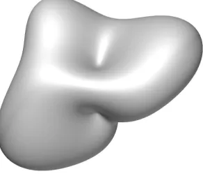
For our first example, we choose the manifold Ω to be the unit sphere in R3 defined byx2+y2+z2= 1. As a test function, we take the function
f1(x, y, z) := 1 +x8+e2y 3
+e2z2+ 10xyz
used in the examples in [1]. As in [1], we visualize this function as a kind of offset surface to the manifold, i.e., we plot
{ξ+f1(ξ)nξ : ξ∈Ω},
[image:9.595.237.383.383.509.2]wherenξ denotes the unit outer normal to the manifoldΩatξ, see Figure 2.
Fig. 2.Test functionf1 on the sphere.
In order to study the behavior of the error as a function of mesh size, we use the nested sequence of triangulations introduced in [1]. LetT0be the regular octahedron with vertices at±ei,i= 1,2,3, whereeiare the Cartesian coordinate vectors. This triangulation has 6 vertices and 8 triangles. We now define Tn by repeated refinement, where Tn is obtained from Tn−1 by adding vertices at the midpoints of the great circle arcs connecting neighboring vertices of Tn−1, and then splitting each triangle inTn−1 into four subtriangles using these new vertices. The number of vertices of Tn is Vn = 22n+2+ 2, and the number of triangles is 22n+3. The triangulations
Fig. 3.TriangulationsT1 andT2.
thatT0is not sufficiently fine for our Powell-Sabin interpolant to be defined, see Section 3.1.
To get test data, we use a simple spherical random number generator, see Remark 6. In particular, for each n= 1,2, . . . ,6, we generate 3Vn = 3(22n+2+ 2) random points. We choose this number since as shown in Section 3.1, the Powell-Sabin interpolant is uniquely defined by 3Vndegrees of freedom. We then evaluate the test functionf1at these points, and create approximantssn by the two-stage method described in Section 3.2.
In the first stage we use least squares multiquadric fitting as described in [6] with the following parameter values: minimum number of points Mmin = 25, maximum number of points Mmax = 100, separation S = 35, and scaling
δ = 0.2 if n = 1, δ = 1.0 if n = 2, δ = 2.0 if n = 3, δ = 3.0 if n ∈ {4,5},
δ = 4.0 if n= 6. See [6] for the exact meaning ofMmin, Mmax, S and δ. The choice of increasing values for the δ’s as the number of data points increases is motivated by numerical results in [6]. In our implementation we make use of the corresponding subroutines from the software library TSFIT [9].
The results of our experiments are presented in Table 1. In the column la-belled Two Stage, we list the relative maximum errors kf1−snk∞/kf1k∞ for
n= 1, . . . ,6. For comparison purposes, in the column labelledExact, we list the relative errors when the exact function values and projected gradients are used instead of the approximate values obtained from first stage fitting. In the column labelledSpherical PS we also list the relative errors corresponding to using the spherical Powell Sabin interpolant of [1] based on the exact function values and gradients at the vertices ofTn.
The table shows that the errors for the three methods are comparable, and indeed for n ≥ 2 are almost identical. To test the rate of convergence, in the column labelled Ratio we list the ratios of the errors of our two-stage method, i.e., kf1−sn−1k/kf1−snk for n = 2, . . . ,6. Since the mesh size decreases by approximately 1/2 at each refinement step, and since the error should be of size
Table 1.Tests with random data on the sphere.
# data Two Stage Ratio Exact Spherical PS T1 54 2.74×10−
1
8.08×10⁻² 7.83×10⁻² T2 198 2.15×10−
2
12.7 2.17×10⁻² 2.10×10⁻² T3 774 2.10×10−
3
10.2 2.10×10⁻³ 2.05×10⁻³ T4 3078 2.41×10−
4
8.7 2.41×10⁻⁴ 2.28×10⁻⁴ T5 12294 2.92×10−
5
8.3 2.92×10⁻⁵ 2.88×10⁻⁵ T6 49158 3.65×10−
6
8.0 3.65×10⁻⁶ 3.60×10⁻⁶
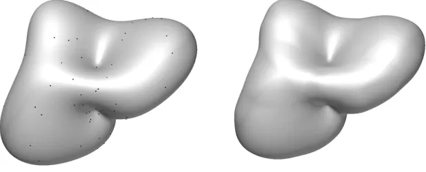
To illustrate the performance of the two-stage method with even fewer data points, we recomputed the spline fit corresponding to the triangulationT2, but with only 100 random points on the sphere. The parameters for the first step were taken to be Mmin = 25, Mmax = 100, S = 25 and δ = 0.8. In this case the maximum relative error was 2.18×10⁻². Figure 4 shows the test function
f1along with the data sites and the approximant computed using the two-stage method.
Fig. 4.Test function with 100 data sites (left) and its approximation (right).
4.2 Ring type surfaces
As a second example, we consider the ring-type surfaces used in the examples presented in [25]. Given a real number 0 ≤ a < 1 and an integer m ≥ 0, we define a smooth 2-manifold inR3 parametrically via
x= [2 + (1 +acosmu) cosv] cosu, (11)
y= [2 + (1 +acosmu) cosv] sinu, (12)
[image:11.595.153.462.349.474.2]where (u, v) runs over the parameter domain [0,2π)×[0,2π). Whenm= 0, this corresponds to a torus with outer radius 3 +aand inner radius 1−a. In general it is a surface of genus 1.
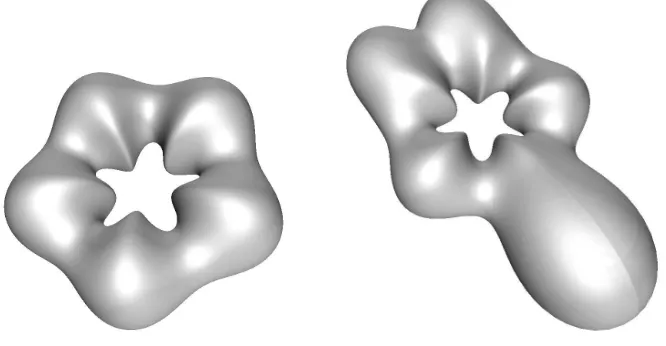
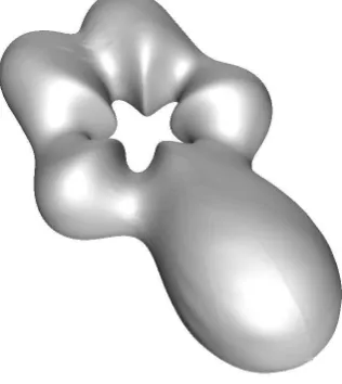
For our experiments, we choosea= 0.3 andm= 5, giving rise to the manifold depicted in Figure 5 (left). As a test function, we now take
f2(x, y, z) := (1 +x8+y3+z2)/4000.
[image:12.595.141.474.253.426.2]The corresponding surface is shown in Figure 5 (right).
Fig. 5. Ring-type surface with a = 0.3 and m = 5 (left), and the test function f2
visualized as an offset surface (right).
For comparison purposes, we generate a sequence of triangulationsTn,n= 1, . . . ,5, by starting with nested three directional meshes in the parameter do-main [0,2π)×[0,2π) with vertices (ui, vj) given by
ui= 2πi
24·2n−1, vj= 2πj
15·2n−1,
and mapping these vertices onto the ring-type surface. The triangulations T1 and T2 are shown in Figure 6. The number of vertices of Tn is Vn = 90·4n, and the number of triangles is 180·4n. To generate data for our experiments, we evaluate the test function f2 at 3Vn random points on the surface. As in Section 4.1, we use local multiquadric fitting [6] with the following parameter values: Mmin = 25, Mmax = 100, S = 15, and δ = 2.0 if n = 1, δ = 3.0 if
Fig. 6.TriangulationsT1 andT2.
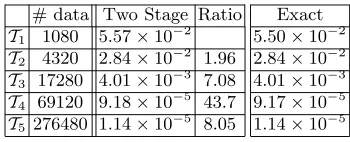
Table 2.Tests with random data on the ring type surface.
# data Two Stage Ratio Exact T1 1080 5.57×10−
2
5.50×10⁻² T2 4320 2.84×10−
2
1.96 2.84×10⁻² T3 17280 4.01×10−
3
7.08 4.01×10⁻³ T4 69120 9.18×10−
5
43.7 9.17×10⁻⁵ T5 276480 1.14×10−
5
8.05 1.14×10⁻⁵
’ratio’ column is probably due to the fact that we are using easy to generate triangulations that are not well adapted to this particular manifold.
Figure 7 shows the T2-approximation computed using 1000 random data, with parametersMmin = 25,Mmax = 100, S = 15, and δ = 2.0. The relative error of this approximation is 2.89×10⁻².
5
Remarks
Remark 1. The problem of fitting functions defined on surfaces arises in many
applications, see [1–4, 10–14, 19, 20, 23, 25, 27, 29], and references therein. Used parametrically, such functions can be applied to the problem of modelling sur-faces of arbitrary topological type from point clouds, see [15, 16, 30].
Remark 2. Many of the papers mentioned in the above remark deal with the
sphere in R3. For a survey of interpolation and scattered data fitting methods on the sphere, see [12]. For some specific methods, see [14, 19, 20, 22, 23, 27, 29].
Remark 3. The method of this paper is closely related to work of Demjanovich
[image:13.595.219.394.313.384.2]Fig. 7.Powell-Sabin approximation computed using 1000 data points.
Γξ determined by the finite element scheme, whereas in our methods we only interpolate projected gradients corresponding to the vertices of the underlying triangulationT, compare steps 3 and 4 of Algorithm 1. Therefore, our interpo-lation operator only requires function values and gradients at the vertices ofT, which makes it possible to design a two-stage scattered data fitting method. In [10, 11] only interpolation with Courant hat functions has similar properties for general manifolds, but it does not produce a C1 interpolant.
Remark 4. The method of this paper is also closely related to work of Pottmann
[25], which also makes use of projected gradients. (It is not difficult to see that our equation (6) describes the π-transform of [25].) However, instead of using local approximation methods to estimate gradients, he constructs a kind of minimum norm network.
Remark 5. Here we have made use of the standard bivariateC1quadratic
Powell-Sabin macro-element to solve the interpolation problem in the tangent plane. Its key feature is that it is constructed from only nine pieces of data, the values and gradients at the three vertices of the macro-triangle. Using the same data, we can also construct an interpolant based on the classicalC1 reduced
Clough-Tocher macro-element. It is based on a split of the macro-triangle into three
subtriangles (typically using the barycenter), and is a cubic polynomial on each piece. Along each edge its cross derivative is restricted to be a linear polynomial. Yet another possibility is a modified quadraticPowell-Sabin macro-element on a
12-split [26], where the cross derivatives are assumed linear rather than piecewise
Remark 6. To simulate scattered data for our numerical experiments in Sec-tion 4, we generated pseudo-random points uniformly distributed on the test surfaces. For the surface of the sphere we use the following method described e.g. in [24]: To obtain a point (x, y, z) on the unit sphere, generate two pseudo-random real numberszandtuniformly distributed in [−1,1] and [0,2π), respec-tively, and then compute x= ρcost and y =ρsint, where ρ= √1−z2. For
the ring-type surface defined parametrically by (11)–(13), the points r(u, v) =
(x(u, v), y(u, v), z(u, v)) will be uniformly distributed on the surface if (u, v)∈ [0,2π)×[0,2π) are chosen according to the probability distribution p(u, v) =
αkru×rvk2, with α∈Rsuch that R[0,2π)×[0,2π)p(u, v)du dv= 1. It is not diffi-cult to see thatkru×rvk22=ψ2[(ψ′)2+(2+ψcosv)2], whereψ(u) = 1+acosmu. Using this explicit formula, we employ the well-known von Neumann rejection method to generate the points.
References
1. P. Alfeld, M. Neamtu and L. L. Schumaker, Fitting scattered data on sphere-like surfaces using spherical splines,J. Comp. Appl. Math.73(1996), 5–43.
2. R. E. Barnhill and T. A. Foley, Methods for constructing surfaces on surfaces,in
“Geometric Modeling: Methods and Their Applications”, Springer, Berlin, 1991, pp. 1–15.
3. R. E. Barnhill, B. R. Piper and S. E. Stead, A multidimensional surface problem: pressure on a wing,Comput. Aided Geom. Design2(1985), 185-187.
4. R. E. Barnhill and H. S. Ou, Surfaces defined on surfaces,Comput. Aided Geom. Design 7(1990), 323-336.
5. O. Davydov, R. Morandi and A. Sestini, Local hybrid approximation for scattered data fitting with bivariate splines,Comput. Aided Geom. Design23(2006), 703–721. 6. O. Davydov, A. Sestini and R. Morandi, Local RBF approximation for scattered data fitting with bivariate splines,in“Trends and Applications in Constructive Ap-proximation,” (M. G. de Bruin, D. H. Mache, and J. Szabados, Eds.), ISNM Vol. 151, Birkh¨auser, 2005, pp. 91–102.
7. O. Davydov and L. L. Schumaker, Interpolation and scattered data fitting on man-ifolds using projected Powell-Sabin splines, manuscript, 2007.
8. O. Davydov and F. Zeilfelder, Scattered data fitting by direct extension of local polynomials to bivariate splines,Advances in Comp. Math.21(2004), 223–271. 9. O. Davydov and F. Zeilfelder, TSFIT: A Software Package for Two-Stage Scattered
Data Fitting, 2005, available under GPL from http://www.maths.strath.ac.uk/ ∼aas04108/tsfit/
10. Yu. K. Demjanovich, Construction of spaces of local functions on manifolds,
Metody Vychisl.(1985) no. 14, 100–109.
11. Yu. K. Demjanovich, Local approximations of functions given on manifolds,Amer. Math. Soc. Transl. (2)159(1994), 53–76.
12. G. Fasshauer and L. L. Schumaker, Scattered data fitting on the sphere,in “Math-ematical Methods for Curves and Surfaces II”, M. Dæhlen, T. Lyche, and L. L. Schumaker (eds.), Vanderbilt University Press, Nashville, 1998, 117–166.
14. W. Freeden, Spherical spline interpolation-basic theory and computional aspects,
J. Comp. Appl. Math. 11(1985), 367–375.
15. C. M. Grimm and J. F. Hughes, Modeling surfaces of arbitrary topology using manifolds,in“Proceedings of SIGGRAPH 95,” 1995, pp. 359–368
16. Xianfeng Gu, Ying He, and Hong Qin, Manifold splines,in“Proceedings of ACM Symposium on Solid and Physical Modeling,” 2005, pp. 27-38.
17. M. W. Hirsch, Differential Topology, Springer-Verlag, 1976.
18. M.-J. Lai and L. L. Schumaker, Spline Functions on Triangulations, Cambridge University Press, Cambridge, 2007.
19. C. L. Lawson, C1
surface interpolation for scattered data on a sphere, Rocky Mountain J. Math.14(1984), 177–202.
20. T. Lyche and L. L. Schumaker, A multiresolution tensor spline method for fitting functions on the sphere,SIAM J. Sci. Computing22(2000), 724–746.
21. C. R. F. Maunder, Algebraic Topology, Van Nostrand Reinhold Company, London, 1970.
22. M. Neamtu and L. L. Schumaker, On the approximation order of splines on spher-ical triangulations,Adv. in Comp. Math.21(2004), 3–20.
23. G. M. Nielson and R. Ramaraj, Interpolation over a sphere based upon a minimum norm network,Comput. Aided Geom. Design4(1987), 41–58.
24. J. O’Rourke, Computational Geometry in C (2nd Ed.), Cambridge University Press, 1998.
25. H. Pottmann, Interpolation on surfaces using minimum norm networks,Computer Aided Geometric Design9(1992), 51–67.
26. M. J. D. Powell and M. A. Sabin, Piecewise quadratic approximations on triangles,
ACM Trans. Math. Software3(1977), 316–325.
27. L. L. Schumaker and C. Traas, Fitting scattered data on spherelike surfaces using tensor products of trigonometric and polynomial splines, Numer. Math.60(1991), 133–144.
28. J. A. Thorpe, Elementary Topics in Differential Geometry, Springer, 1979. 29. G. Wahba, Spline interpolation and smoothing on the sphere,SIAM J. Sci. Stat.
Computing2(1981), 5–16.