Generalised Sharpe Ratios and Asset Pricing in Incomplete Markets

City, University of London Institutional Repository

Citation: Černý, A. (2003). Generalised Sharpe Ratios and Asset Pricing in Incomplete

This is the accepted version of the paper.

This version of the publication may differ from the final published

version.

Permanent repository link: http://openaccess.city.ac.uk/16294/

Link to published version: http://dx.doi.org/10.1023/A:1024568429527

Copyright and reuse: City Research Online aims to make research

outputs of City, University of London available to a wider audience.

Copyright and Moral Rights remain with the author(s) and/or copyright

holders. URLs from City Research Online may be freely distributed and

linked to.

City Research Online: http://openaccess.city.ac.uk/ publications@city.ac.uk

Markets

Aleš µCerný (a.cerny@ic.ac.uk)

Imperial College Management School

First draft: November 1998, this version November 2002

Abstract.

The paper presents an incomplete market pricing methodology generating asset price bounds conditional on the absence of attractive investment opportunities in equilibrium. The paper extends and generalises the seminal article of Cochrane and Saá-Requejo who pioneered option pricing based on the absence of arbitrage and high Sharpe Ratios. Our contribution is threefold:

We base the equilibrium restrictions on an arbitrary utility function, obtaining the Cochrane and Saá-Requejo analysis as a special case with truncated quadratic utility. We extend the de…nition of Sharpe Ratio from quadratic utility to the entire family of CRRA utility functions and restate the equilibrium restrictions in terms of Generalised Sharpe Ratios which, unlike the standard Sharpe Ratio, provide a consistent ranking of investment opportunities even when asset returns are highly non-normal. Last but not least, we demonstrate that for Itô processes the Cochrane and Saá-Requejo price bounds are invariant to the choice of the utility function, and that in the limit they tend to a unique price determined by the minimal martingale measure.

Keywords: Generalised Sharpe Ratio, price bounds, arbitrage, good deal, incom-plete market, certainty equivalent, reward for risk measure, optimal portfolio, duality and martingale methods, minimal martingale measure

JEL classi…cation code:G12, D40, C61

1. Introduction

Asset pricing in incomplete markets is an intriguing problem because of the price ambiguity one has to deal with. Traditionally this ambi-guity is either removed completely by assuming a representative agent equilibrium or it is acknowledged in its fullest by looking at the no-arbitrage bounds. Arguably the former assumption is too strong and the latter assumption is too weak. Good-deal pricing introduces moderately

strong equilibrium restrictions somewhere between the two extremes, postulating the absence of attractive investment opportunities – good deals – in equilibrium. Under the in‡uence of CAPM and APT attrac-tive investments became associated with high Sharpe Ratios, both in theoretical and empirical work (Ross (1976), Shanken (1992), Cochrane and Saá-Requejo (2000)), but µCerný and Hodges (2001) show that one can impose the good-deal restrictions with considerable generality. The generic term ‘good deals’ was introduced by Cochrane and Saá-Requejo (2000) who were the …rst to successfully apply the good-deal restric-tions to option pricing. The idea of Cochrane and Saá-Requejo was to restrict the availability of high Sharpe Ratios at every point in time. Using the dual discount factor restrictions and backward recursion they calculated option price bounds that are based on very believable equilibrium restrictions, yet are much narrower than the corresponding super-replication bounds.

The association of good deals with high Sharpe Ratios has its pit-falls. High Sharpe Ratios do not include all arbitrage opportunities, therefore to make the equilibrium restrictions meaningful one must eliminate not just high Sharpe Ratios (grey circle in Figure 1) but also arbitrage opportunities (dark triangle) and all the convex combinations between the two types of investments (black contour). As a result the

Figure 1. Black contour contains the set of good deals generated as a combination of high Sharpe Ratios (grey circle) and arbitrage opportunities (dark grey triangle).

equilibrium restriction of Cochrane and Saá-Requejo cannot be de-scribed by imposing restrictions on the standard Sharpe Ratio alone, but as we show here it is associated to a level of theArbitrage-Adjusted Sharpe Ratio discussed in section 3.1.

one-to-one relationship between the maximum quadratic utility attainable in a market and the market Sharpe Ratio. Crucially, Sharpe Ratio re-labels the levels of quadratic utility in such a fashion that the labels do not depend on the initial wealth.

The relationship with quadratic utility explains why Sharpe Ratio is

not a good reward-for-risk measure. Quadratic utility has a bliss point, one is penalised for achieving wealth beyond this point. Consider two assetsAandBwith excess returns given in Table I. The optimal wealth

Table I. AssetAstochastically dominated by assetB Probability 1

6 1 2

1

3 Sharpe Ratio

Return of Asset A -1% 1% 2% 1.0 Return of Asset B -1% 1% 11% 0.8

in marketA does not extend beyond the bliss point, whereas in market

B it does. This is why asset A achieves a higher Sharpe ratio of 1.0 than the unambiguously more attractive assetB(SR of 0.8). To obtain meaningful price bounds based on Sharpe ratio one must prevent such anomalous behaviour. The remedy is to make the utility non-decreasing after the bliss point – hence the need for truncated quadratic utility. The resulting wealth-independent labelling of the levels of truncated quadratic utility leads to the Arbitrage-Adjusted Sharpe Ratio. The Cochrane and Saá-Requejo set of good deals is simply the set of excess returns with high Arbitrage-Adjusted Sharpe Ratio.

Since truncated quadratic utility has none of the tractability of its non-truncated counterpart, it is natural to ask whether other utility functions are a viable alternative. For a given candidate utility function this means …rstly de…ning the corresponding Generalised Sharpe Ratio, and secondly computing so called ‘discount factor restrictions’ corre-sponding to that GSR. For example, the Cochrane and Saá-Requejo set of equilibrium pricing kernels must satisfy Var(m)_·h2

Awheremis the pricing kernel andhAis the upper bound on Arbitrage-Adjusted Sharpe Ratio. Our …rst contribution is in showing how to derive this duality restriction for an arbitrary utility function. The second contribution is in extending the de…nition of the Sharpe ratio from quadratic utility to the entire CRRA family of utility functions and showing how such extension can, in principle, be performed for any utility function.

Föllmer and Schweizer (1989), closely related to thenumeraire portfolio

of Long (1990), see also µCerný (1999) and Kallsen (2002).

As an answer to ‘What are the discount factor restrictions implied by standard utility functions?’ we can o¤er the following:

1. Truncated quadratic utility

1 +h2_A(basis)_·Ehm2i_·1 +h2_A (1)

2. Negative exponential (CARA) utility

1 2h

2

E(basis)·E [mlnm]·

1 2h

2

E (2)

3. CRRA utility0< ° ₆= 1;and truncated CRRA utility° <0

³

1 +h2_°(basis)´ 1¡°

2°2

·Ehm1¡°1i_·³_{1 +h}2

°

´1¡°

2°2

(3)

Truncated quadratic is a special case with°=_¡1,h_¡1 =hA. 4. Logarithmic utility°= 1

ln³1 +h2₁(basis)´_{· ¡}2E [lnm]_·ln³1 +h2₁´ (4)

where m > 0 is the change of measure, hA is the Sharpe Ratio adjusted for arbitrage, hE;andh° are the Generalised Sharpe Ra-tios generated by the CARA and CRRA utility, respectively. All variables with attribute ‘basis’ refer to the market containing only basis assets (that is without focus assets to be priced).

5. For Itô price processes the instantaneous restrictions coincide for all utility functions. Denotingº the market price of risk vector, the no-good-deal restriction becomes

h2(basis)_{· jj}º_jj2 _·h2.

For each of the utility functions in (1)-(4) the two inequalities are a direct consequence of the Extension Theorem, familiar from no-arbitrage pricing1_{. The left hand side inequalities are known in …nancial}

litera-ture, although the authors do not seem to be aware of the common principle underlying all of them. These restrictions have been used to diagnose asset pricing models, and correspond to the above utility functions as follows

1

1. Hansen and Jagannathan (1991), Hansen et al. (1995),

2. Stutzer (1995),

3. with0< °₆= 1Snow (1991), and

4. Bansal and Lehmann (1997).

The economic interpretation of the left hand side inequalities in (1)-(4) is simple: the best deal in a market containing only basis assets cannot be better than the best deal in a market including also the focus asset. The genuine no-good-deal restrictions are the right hand side inequalities, which quantify by how much the best deal can improve after the introduction of a focus asset. Here the only representative was the restriction (1) of Cochrane and Saá-Requejo (2000).

The Generalised Sharpe Ratios in (1)-(4) provide a scale-free mea-sure of risk which behaves like the standard Sharpe Ratio for excess returns with small dispersion. We derive simple formulae that permit calculation of Generalised Sharpe Ratios for an arbitrary vector of excess return X: In the case of CRRA family of utility functions we have

h2_°(X) =

µ

max

¸ E

h

(1 +¸X)1¡°i¶ 2°

1¡°

¡1 for0< ° <1 (5)

h2_°(X) =

µ

min

¸ E

h

(1 +¸X)1¡°i¶ 2°

1¡°

¡1 for1< ° (6)

h2_°(X) =

µ

min

¸ E

h

max (1 +¸X;0)1¡°i¶ 2°

1¡°

¡1 for° <0 (7)

h2_°(X) =e2 max¸E[ln(1+¸X)]_{¡1 for°= 1: (8)}

To obtain the Arbitrage-Adjusted Sharpe Ratio one computesh_¡1 in

equation (7), to obtain thestandard Sharpe Ratio2 one simply removes the truncation at zero in the de…nition ofh_¡1,

h2(X) =

µ

min

¸ E

h

(1 +¸X)2i¶

¡1

¡1: (9)

2 _{Since its …rst appearance in Sharpe (1966) there has been a number of}

The Generalised Sharpe Ratios proposed in this paper can be used with great advantage in portfolio management, because unlike the stan-dard Sharpe Ratio they provide a consistent ranking of investment opportunities when asset returns are highly skewed.

Bernardo and Ledoit (2000) propose to base the de…nition of good deals on the gain-loss ratio. This reward-for-risk measure cannot be captured in our framework, for the following reason. In the present paper we …x the utility function and we measure good deals by the (appropriately rescaled) levels of expected utility. Bernardo and Ledoit, on the other hand, …x the level of expected utility that de…nes a good deal and they rank the good deals by changing theshape of the utility function. Namely, the gain-loss ratio is based on the Domar-Musgrave utility. With a piecewise linear utility in a frictionless market the maxi-mum expected utility of a risky investment is either zero or plus in…nity, and one can a¤ect the outcome by changing the ratio of the slopes of the two linear parts of Domar-Musgrave utility function. The slope ratio at which expected utility switches from 0 to +₁ is the market gain-loss ratio. The discount factor restrictions are similar in nature to those mentioned above

Lbasis ·

ess supm

ess infm ·L;

whereLdenotes the maximum loss ratio in the market. The gain-loss does not work well in Itô process environment with continuous trading where typicallyLbasis = +1;as in, for example, the standard

Black-Scholes model.

1.1. Organisation of the paper

The second section discusses one-period no-good-deal equilibria and the corresponding discount factor restrictions. The third section de-scribes the link between the certainty equivalent gains and (Gener-alised) Sharpe Ratios; in particular it extends the de…nition of Sharpe Ratio to the entire family of CRRA utility functions. Section four gives two numerical examples which illustrate the computation of option price bounds in multiperiod model based on a number of Generalised Sharpe Ratios.

2. No-good-deal restrictions in one-period model

Consider a market with a …nite number of states. Let r be the risk-free rate of return and let X be the vector of excess returns of basis risky assets. Byµdenote the portfolio of basis assets. For a …xed utility function and …xed initial endowment V0 it is natural to measure the

attractiveness of a self-…nancing investment by thecertainty equivalent

of the resulting wealthV relative to the wealth of a riskless investment into the bank account. Speci…cally, the value of the best deal in a market characterised by excess return X will be denoted a(X);with

a(X) de…ned implicitly as follow

U[(1 +r)V0+a(X)],sup

µ

E [U((1 +r)V0+µX)], (10)

having substituted for V from equation (40). The fact that the cer-tainty equivalent a(X) depends on V0 is a nuisance, but it allows us

to formulate and solve the pricing problem for any utility function,

therefore formulation (10) is the most convenient at this point. Section 3 discusses the link between the certainty equivalent gain a(X) and Generalised Sharpe Ratios.

Consider a focus assetY:By P₁(Y)we will denote the no-arbitrage price range of Y. Taking a …xed upper bound ¹a, we de…ne the set of no-good-deal equilibrium prices ofY as

P¹a(Y),fpyja(X; Y ¡(1 +r)py)·¹ag \P1(Y): (11)

Before we give a full characterisation of no-good-deal price bounds in …nite dimension (Theorem 2), it is useful to provide the following classi…cation of utility functions

DEFINITION 1. Let U(x) be a non-decreasing concave function de-…ned on an interval _D= (c;+₁); _{¡1 ·}c <+₁. We will distinguish the following three cases

U1) U(x) is unbounded from above (and necessarily strictly increasing on_D):

U2) U(x) is bounded from above and strictly increasing on _D.

U3) U(x) is bounded from above and there is a threshold x¹ _{2 D} such thatU(x) is constant for x_¸x¹ and U(x) is strictly increasing for x_{2 D}such thatx <x. In this case we assume¹ (1+r)V0 <x¹;utility

THEOREM 2. Assume that utility function U(:) is non-decreasing, di¤erentiable and that it satis…es

lim

x!¡1

x U(x) = 0:

Assume further that there is no arbitrage among the basis assets. Then

1. The a(X) The supremum in (10) is …nite and it is attained by at least one portfolio µ: Moreover, the corresponding certainty equiv-alenta(X) is …nite. Let us denote its value by abasis.

2. For any focus asset Y the setP¹a(Y) is empty for ¹a < abasis and it

is a non-empty interval for ¹a > abasis:

3. In cases U1), U2) Pabasis(Y) is non-empty, in case U3) Pabasis(Y) may be empty.

4. For ¹a > abasis P¹a(Y) contains a single point if and only if Y is a

redundant asset (there is µ such thatY =const+µX).

5. If abasis ·a1 < a2 and Y is non-redundant then Pa1(Y) is inside

Pa2(Y)which in turn is insideP1(Y)(the no-arbitrage price region

for Y): If Pa2(Y) is strictly inside P1(Y) then Pa1(Y) is strictly

inside Pa2(Y): In the case U1) Pa2(Y) is always strictly inside

P₁(Y):

6. Asa2 tends to in…nityPa2(Y)tends to the no-arbitrage price range,

mathematically

[

a2

Pa2(Y) =P1(Y): (12)

7. The no-arbitrage restriction in (11) is cosmetic in the following sense. If p _{2 f}pyja(X; Y ¡(1 +r)py) · ¹ag then p 2 clP1(Y);

that is only the end points of_fp_yja(X; Y _¡(1 +r)py)·¹ag may lie

outside the no-arbitrage bounds and this may only happen in the cases U2), U3).

Proof: See Appendix A.

With a bounded utility function it may happen that the no-good-deal price regionP¹a(Y) hits one or both no-arbitrage bounds for …nite¹a;in such caseP¹a(Y)does not grow further beyond the no-arbitrage bounds as¹aincreases.

In the rest of this section we will proceed in 2 steps. First we will explain how to …nd the highest a attainable in a complete market. In the second step we will show how, with the help of an extension theorem, this information can be used to …nd the no-good-deal price of an arbitrary focus asset. The second step will in a natural way lead to the dual discount factor restrictions.

Suppose the market X is complete and the state prices are given by a unique change of measure m; our aim is to …nd the maximum certainty equivalent gain a(m) in this market. Instead of looking for the optimal investment strategy µ we will use an elegant trick, due to Pliska (1986), of searching for the optimal distribution of wealth, subject to the budget constraint dictated by the state pricesm

max

µ E [U((1 +r)V0+µX)] = maxV

s.t.E[mV]=(1+r)V0

E [U(V)];

whereby fora(m)we simply have

U[(1 +r)V0+a(m)], max

V

s.t.E[mV]=(1+r)V0

E [U(V)]: (13)

In a …nite state model the maximisation problem (13) is standard. Since there is just one linear constraint one solves (13) using unconstrained maximisation separately in each state with a Lagrange multiplier

max

V(!)

!2­

U(V(!))_¡¸m(!)V(!):

The …rst order conditions give

U0(V(!)) =¸m(!)

Denoting I(:) the inverse function to the marginal utility U0(:) we obtain

V =I(¸m) (14)

and from the restrictionE [mV] = (1 +r)V0 we can recover the value

As an example let us apply the above procedure to the negative exponential utility. First we …nd the inverse of the marginal utility

U(V) = _¡e¡AV U0(V) = Ae¡AV

I(x) = _¡1

Aln x A:

The optimal terminal wealth is then

V =I(¸m) =_¡1

Aln ¸m

A :

We recover the Lagrange multiplier from the budget constraint and plug this value back into the expression for optimal wealth

E [mV] = (1 +r)V0

¸=Ae¡A(1+r)V0¡E[mlnm]

V = (1 +r)V0+ E ·_m

A ln m A

¸

¡_A1 lnm

A:

Finally, we recover the certainty equivalent of the optimal risky invest-ment

U(V) =_¡me¡A(1+r)V0¡E[mlnm] E [U(V)] =_¡e¡A(1+r)V0¡E[mlnm]

a(m) =U¡1(E [U(V)])_¡(1 +r)V0=

1

AE [mlnm]: (15)

2.1. Discount factor restrictions in good-deal pricing

We have just seen how one calculates the maximum attainable certainty equivalent a(m) in a complete market. The crucial link between the complete and incomplete market is provided by theextension theorem3 which asserts that any incomplete market without good deals can be embedded in a complete market that has no good deals. Let us denote by abasis the certainty equivalent of the best deal attainable in the market containing only the basis assets:Two observations follow from the extension theorem. The best deal in the completed market cannot

3 _{Interestingly, both the idea of Sharpe Ratio restrictions and the use of the}

be worse than the best deal in the original market containing only basis assets:On the other hand, for any " >0 there is no good deal of size

abasis+"in the market containing just basis assets. Consequently, by extension theorem there must be a completion with a pricing kernelm

for whicha(m)< abasis+":By letting "!0we obtain

abasis = inf_m a(m)

wheremmust price correctly all basis assets. This argument is inspired by ‘…ctitious completions’ of Karatzas et al. (1991). In a …nite state model the in…mum is always attained by at least one pricing kernel.

THEOREM 3. Assume that utility functionU(:) satis…es

lim

x!¡1

x U(x) = 0:

If there is no arbitrage among the basis assets then we have the following dual characterisation of good-deal price bounds:

1. In the cases U1, U2 for ¹a_¸abasis

P¹a(Y) =

½_{E [mY]}

1 +r

¯ ¯ ¯

¯abasis ·a(m)·¹a;E [mX] = 0; m >0

¾

: (16)

Furthermore, for unbounded utility (U1) m > 0 in (16) can be omitted.

2. In the case U3 for ¹a_¸abasis and Y non-redundant de…ne

~

Pa¹(Y) ,

½_{E [mY]}

1 +r

¯¯ ¯

¯abasis ·a(m)·a;¹ E [mX] = 0; m¸0

¾

;

P₁(Y) = (p_¡1; p₁);p_¡1< p₁ Then

P¹a(Y)µP~¹a(Y)µP¹a(Y)[ fp¡1g [ fp1g: (17)

Proof: See Appendix A.

The restrictions of the type abasis ·a(m) are well known in …nan-cial economics, where they have been employed to test di¤erent asset pricing models4. We are, however, primarily interested in the pricing

4

implications of the extension theorem. Suppose that we want to …nd all prices of a focus asset that do not provide good deals of size ¹a in the enlarged market. From the extension theorem all such prices must be supported by pricing kernels for whicha(m) _·¹a: This is the dual no-good-deal discount factor restriction.

For example, for the CARA utility we have from (15) Aa(m) = E [mlnm]and therefore the discount factor restrictions read

Aabasis·E [mlnm]·A¹a (18)

E [mX] = 0; m >0:

In conclusion, the market including both basis and focus assets does not provide deals better than¹a; as measured by CARA utility, if (and only if) the focus assets are priced with no-arbitrage pricing kernels consistent with basis assets and satisfying the restriction (18).

Below we summarise the no-good-deal restrictions on the change of measure m for standard utility functions. The derivation proceeds as explained above between equations (13) and (15).

1. Truncated quadratic utility U(V) = _¡( ¹V _¡V)2 ; V < V¹ and

U(V) = 0 ;V _¸V¹

µ ₁

1_¡Aabasis

¶2

·Ehm2i_·

µ ₁

1_¡Aa

¶2

(19)

2. Negative exponential utilityU(V) =_¡e¡AV

Aabasis ·E [mlnm]·Aa (20)

3. Power (isoelastic) utilityU(V) = V₁1_¡¡_°° ;0< °₆= 1; V >0

µ

1 +Aabasis

°

¶1

°¡1

·Ehm1¡°1i_·

µ

1 +Aa

°

¶1

°¡1

(21)

4. Logarithmic utilityU(V) = lnV; V >0

ln (1 +Aabasis)· ¡E [lnm]·ln (1 +Aa): (22)

3. Generalised Sharpe Ratios

Having derived the state price restrictions (19)-(22) the task changes into interpreting the state price bounds as reward for risk measures, preferably ones that are close in nature to Sharpe Ratio. Note that if one usesa as the measure of attractiveness then one has to specify the coe¤cient of absolute risk-aversion in restrictions (19)-(22). It turns out that for small Sharpe Ratios there is an unambiguous link between Sharpe Ratios and certainty equivalent gains, which we describe next. To keep technicalities at minimum we assume that the excess return

X has bounded support and that the utility function is su¢ciently di¤erentiable. From the Taylor expansion we obtain

E [U(V0+µX)] = U(V0) +U0(V0)µE [X] +

+1 2U

00_(V

0)µ2E h

X2i+o(µ2EhX2i)

and after maximisation with respect toµwe will have

^

µ = U

0_(V

0)E [X]

U00_{(V0)E [X}2_]+o

µ_{E [X]}

E [X2_] ¶

max

µ E [U(V0+µX)] = U(V0)¡

1 2

(U0(V0)E [X])2

U00_{(V0)E [X}2_] +o Ã

(E [X])2 E [X2_]

!

. (23)

Without loss of generality we can assume thatX_E[E[_XX2]_]is small for all

re-alisations ofXso that the Taylor series approximation ofU³V0+ ^µX ´

can be made arbitrarily precise. At the same time, for a small certainty equivalent gain we can write

U(V0+a) =U(V0) +U0(V0)a+o(a); (24)

and the comparison of (23) and (24) gives

a= h

2_(X)

2A(V0)

+o(h2) (25)

whereA(V) =_¡U_U00₀₍(_VV₎) is the coe¢cient of absolute risk-aversion,h(X)

is the Sharpe ratio ofX

h(X), q E [X]

E [X2_{]¡(E [X])}2

;

andlim_h2_!0 o(h 2₎

In conclusion, one could replace Aa in expressions (19)-(22) with h2

2 . Naturally, this is not the only transformation that satis…es the

asymptotic property (25). For example, for small values ofh2 we have

h2= h

2

1 +h2 +o(h

2_{) =e}h2

¡1 +o(h2);

and indeed we might equally well replaceAa with any other function

f(h2)as long asf is continuously di¤erentiable around0withf(0) = 0

and f0(0) = 1₂. The rest of this section describes how the ambiguity in choosing the function f(h2) is resolved for negative exponential, truncated quadratic and CRRA utility.

3.1. Truncated quadratic utility

To begin with, consider maximisation ofnon-truncated quadratic util-ity for a single asset with excess returnX;

max

µ ¡E

h

(1_¡µX)2i:

The optimal investment is

^

µ= E [X]

E [X2_] (26)

and the maximum utility is an increasing function of the Sharpe Ratio

max

µ ¡E

h

(1_¡µX)2i= (E [X])

2

E [X2_] ¡1 =¡

1

1 +h2_(X); (27)

or conversely

h2(X) = 1 minµE

h

(1 +µX)2i¡

1: (28)

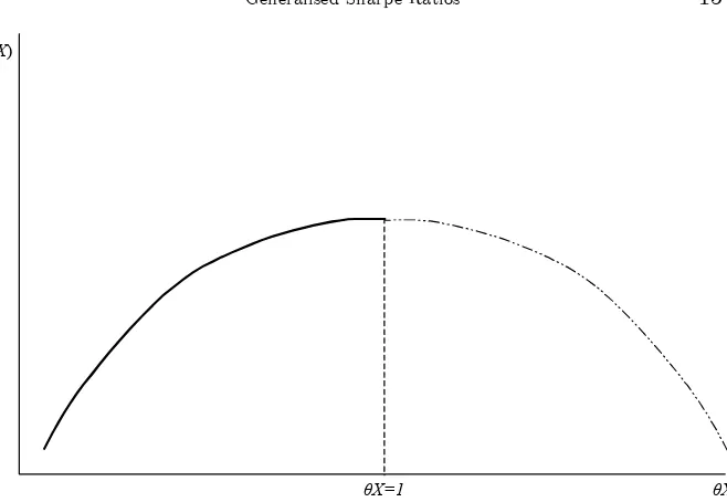
The quadratic utility function has a bliss point at µX = 1; having more wealth than 1 actually lowers the expected utility. The optimal wealth will not extend beyond the bliss point if and only if ^µX _· 1;

that is if

xmaxE [X]·E h

X2i; (29)

wherexmax,ess supX is the highest excess return. If (29) is violated

θX θX=1

U(θX)

Figure 2. Quadratic utility has a bliss point

away in the states where ^µX >1 the Sharpe Ratio of X will actually increase. More speci…cally, we can replace the original excess return distribution X with a distribution Xcap capped at a …xed value xcap:

Initiallyxcap is set atxmax and condition

xcapE [Xcap]·E h

X_cap2 i (30)

is not satis…ed. By loweringxcap we increase the Sharpe Ratio of the

capped distribution and make the di¤erence between the left hand side and the right hand side in condition (30) smaller. The Sharpe Ratio of the capped distribution reaches its maximum just when

xcapE [Xcap] = E h

X_cap2 i: (31)

At this point we have decomposed X into a pure Sharpe Ratio part

Xcap and the pure arbitrage partX¡Xcap.

Table II. Distribution of excess return

x -1% 1% 11% Pr(X=x) 1

6 1 2

1 3

For the Sharpe Ratio we have

E [X] = 4

Var [X] = 25

6 +

9

2+

49

3 = 25

h(X) = p4

25 = 0:8:

Let us now see whether the bliss point condition (29) is violated. To this end

xmaxE [X] = 11£4 = 44;

whereas

EhX2i= Var [X]_¡(E [X])2 = 25_¡16 = 9;

which means that the condition is indeed violated and one can in-crease the Sharpe Ratio by putting some money aside. Guessing that the truncation point will occur at xcap > 1% we can write the bliss

point condition (31) as

xcap

µ₁

6£(¡1) + 1 2 £1 +

1 3 £xcap

¶

=

µ₁

6 £(¡1)

2₊1

2 £1

2₊1

3 £x

2

cap

¶

:

Solving for xcap we …nd xcap= 2 and

hA(X) = h(Xcap) =

E [Xcap]

r

EhX2

cap

i

¡(E [Xcap])2

=

= q _xcap1 E[Xcap]¡1

= q 1

2 1 ¡1

= 1

The arbitrage-adjusted Sharpe Ratio is 1 compared to the standard Sharpe Ratio of 0:8. The pure Sharpe Ratio part of excess return X is

and the pure arbitrage part is

XA= [0% 0% 9%].

Figure 3 shows a slice of the 3D space of excess returns in the plane x1+x2+x3 = 1; it is, so to speak, bird’s-eye view of the market from

direction (1,1,1). The set of arbitrage opportunities (positive octant) appears as a dark grey triangle, the set of Sharpe Ratios greater than 1.0 appears as the medium grey circle and the Sharpe Ratios greater than 0.8 are inside the outer light grey circle. The decomposition into pure Sharpe Ratio and a pure arbitrage opportunity is captured as a movement from the original excess returnX with low Sharpe Ratio to the truncated excess returnXcap with high Sharpe Ratio, away from the

arbitrage opportunity XA. The Arbitrage-Adjusted Sharpe Ratio of X

is de…ned as the Sharpe Ratio ofXcap.

XA

X

X cap

Figure 3. Illustration to Arbitrage-adjusted Sharpe Ratio: Movement from X to-wardsXcap, away from the arbitrage opportunityXA, leads to higher Sharpe Ratio (circle with smaller radius).

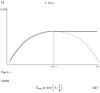
Truncated quadratic utility formalises the ‘throwing money away’ procedure. With truncated utility one is neither rewarded nor penalised for achieving wealth levels above the bliss point, thus the excess return is e¤ectively capped at a level whereµX = 1:

Namely

max

µ ¡E

h

(max(1_¡µX;0))2i= (E [Xcap])

2

EhX2 cap

i ¡1 =_¡ 1 1 +h2_(X

cap)

;

θX θX=1

UTQ(θX)

Figure 4.

where

Xcap= min µ

X;1

^

µ

¶

(33)

with^µ being the optimal portfolio weight in (32). The …rst order con-ditions in (32) correspond exactly to

xcapE [Xcap] = E h

X_cap2 i:

Appendix B shows that the above argument works withE [X]>0. For

E [X] < 0 the value xmax in condition (30) has to be replaced with

xmin´ess infX and the truncation proceeds from below.

We have argued intuitively that the Sharpe Ratio of Xcap is the

arbitrage-adjusted Sharpe Ratio ofX. Equation (32) then suggests how to de…nehA(X)using the truncated quadratic utility

h2_A(X), 1

minµE [max(1 +µX;0)2]¡

1: (34)

The obvious advantage of (34) is that it can be used with multiple assets, whereas the intuition of ‘throwing money away’ only works with one asset.

PROPOSITION 5. The convex hull of _fX_jh(X) _¸ ¹h_g and _fX_jX _¸

0_g coincides with _fX_jhA(X) ¸ ¹hg [ fXjX ¸ 0g: Graphically, if the

medium grey circle in Figure 3 is described by h(X) _¸ ¹h then the area delineated by the black contour in the same Figure is described by hA(X)¸h.¹

Proof. Denote by Bthe convex hull of_fX_jh(X)_¸¹h_g and_fX_jX_¸

0_g; and let C =_fX_jhA(X) ¸h¹g [@fXjX ¸0g: If X 2B then there

isXA¸0 andXh withh(Xh)¸¹hsuch thatX =XA+Xh. By virtue

of (26) and (28)h(Xh)¸¹himplies

¹

h2 _· 1

Eh(1 + ^µXh)2

i¡1

for ^µ = _¡E [Xh] E£X_h2¤:

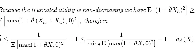
Because the truncated utility is non-decreasing we haveEh(1 + ^µXh)2

i

¸

Ehmax(1 + ^µ(Xh+Xa);0)2

i

, therefore

¹

h_· 1

Ehmax(1 + ^µX;0)2i ¡1·

1

minµE [max(1 +µX;0)2]¡

1 =hA(X)

and we have shownX ₂B₎X₂C:

Conversely, assumeX ₂C:Then either X_{2 f}X_jX_¸0_g (X lies in the positive orthant) and then triviallyX ₂B;or X_{62 f}X_jX _¸0_g and then by virtue of Theorem 2, part 1. there is …nite^µsuch thath2

A(X) =

1

E[max(1+^µX;0)2_] ¡1: By virtue of (32), (33) we obtain a decomposition

X=Xcap+XA such that h(Xcap) =hA(X)¸¹hand XA¸0; proving

thatX₂B:

Table III. Di¤erence betweenhAandhfor lognormal risky return.hA arbitrage-adjusted Sharpe Ratio,h standard Sharpe Ratio,R¹ expected risky return, R

risk-free return,¾return volatility ¹

R R ¾ h hA %error hA_h¡h 1.04 1.02 0.04 0.5 0.502 0.5%

1.06 1.02 0.08 0.5 0.503 0.6%

1.18 1.02 0.16 0.5 0.512 2.4%

1.04 1.02 0.02 1.0 1.085 8.5%

1.06 1.02 0.04 1.0 1.093 9.3%

1.18 1.02 0.08 1.0 1.140 14.0%

1.06 1.02 0.02 2.0 3.675 83.7%

1.10 1.02 0.04 2.0 3.824 91.2%

1.34 1.02 0.08 2.0 4.845 142.3%

3.2. Family of CRRA utility functions

Recall from (21) that the duality between pricing kernels and certainty equivalent gains in this case reads

Et¡1 ·

m1¡

1

°

tjt¡1 ¸

=

µ

1 +Aa

°

¶1

°¡1

: (35)

The asymptotic relationship between certainty equivalent and Sharpe Ratio isAa= h₂2 which yields

Et¡1 ·

m1¡

1

°

tjt¡1 ¸

=

Ã

1 +h

2

°

2°

!1

°¡1

: (36)

By virtue of (25) all the generalised Sharpe Ratios h° de…ned by (36) have the same asymptotic behaviour for small values. It remains to check the consistency of this de…nition with the de…nition of the Arbitrage-Adjusted Sharpe Ratio, for which the duality is

Et¡1 h

m2_tjt¡1i= 1 +h2_A:

Recall that quadratic utility has ° = _¡1; substituting this value into equation (36) we obtain

Et¡1 h

m2_tjt¡1i=

Ã

1_¡ h

2

¡1

2

!¡2

and it is clear that h_¡1 from (36) is not equal to hA even though asymptotically they are the same. Fortunately, there is an easy way out to achieveh_¡1=hA. It is enough to realise that asymptotically

Ã

1 +·h

2 ° 2° !1 · ¡1

°¡1

¢

=

Ã

1 +h

2

°

2°

!¡1

°¡1

¢

+o(h2_°)

for all·:There are many choices of·(°);for example·=_¡2or·= 2°;

such thath_¡1 =hA:A good way to pinpoint the ‘right’ value of·is to look at the time scaling properties of the standard Sharpe Ratio and to compare them with the time scaling properties of the Generalised Sharpe Ratio h°; see Section 6. It turns out that one needs · = 2°: The discount factor restrictions then become

³

1 +h2_°basis´

1¡°

2°2

· E

·

m°¡°1

¸

·³1 +h2_°´

1¡°

2°2 ₍₃₇₎

1 2ln

³

1 +h2_1basis´ _{· ¡}Ehlnmtjt¡1 i

· 1₂ln³1 +h2₁´: (38)

Comparing (37) with (21) and using the de…nition of certainty equiv-alent gain we obtain the computational de…nition of CRRA Sharpe Ratio for a given excess returnX

1 +h2_°(X) =

µ

max

¸ E

h

(1 +¸X)1¡°i¶ 2°

1¡°

for0< ° <1

1 +h2_°(X) = e2 max¸E ln(1+¸X) _{for°= 1}

1 +h2_°(X) =

µ

min

¸ E

h

(1 +¸X)1¡°i¶ 2°

1¡°

for1< °:

These de…nitions naturally extend to ° < 0 if the CRRA utility is truncated at the value of zero

U(V) = _¡

¡_¹

V _¡V¢1¡°

1_¡° forV <V¹ U(V) = 0 forV _¸V¹

1 +h2_°(X) =

µ

min

¸ E

h

max(1 +¸X;0)1¡°i¶ 2°

3.3. Negative exponential utility

Interestingly, there is a special case where the relationship h2 = 2Aa

holds for large certainty equivalent gains. By inverting the no-good-deal restriction (10) for negative exponential utility with an arbitrary random excess returnX one obtains

a(X) =_¡1

Aln

µ

¡max

µ ¡E

h

e¡AµXi¶=_¡1

Aln

µ

min

µ E

h

eµXi¶:

Hodges (1998) points out that for anormally distributed excess return

X we have identically

1 2h

2_{(X) =}

¡ln

µ

min

µ E

h

eµXi¶; (39)

whereh(X)is a standard Sharpe Ratio, and consequently Hodges uses equation (39) to de…ne theGeneralised Sharpe RatiohE for an

arbitrar-ily distributed excess return. The maximum Exponential Sharpe Ratio is hence related to the maximum certainty equivalent gain through (25)

1 2h

2

E =Aa;

and one can write the state price restriction (20) in a scale-free form

1 2h

2

E(basis)·E [mlnm]·

1 2h

2

E:

4. Two numerical examples

4.1. The relationship between one-period and multi-period model

Let us have a …ltered probability space (­;_F;_P;_fFtgt=0;1;::: ;T) with

Et[:]denoting the expectation conditional on the information at time

Let µ be an _Rn-valued portfolio process for ‘risky securities’. If an agent uses self-…nancing strategies her wealthVt evolves over time as follows

Vt = (1 +rt¡1)Vt¡1+µt¡1Xt (40)

Xt = St+Dt¡(1 +rt¡1)St¡1; (41)

where Xt

St¡1 can be interpreted as excess return when St¡1 6= 0. No

arbitrage means that there is a strictly positive_Ft-measurable variable5

m_tjt¡1 withEt¡1 h

m_tjt¡1i= 1such that

Et¡1 h

m_tjt¡1Xt

i

= 0,

that is with arti…cial probabilities de…ned by mtjt¡1 the discounted

wealth process is a martingale betweent_¡1and t

Et¡1 h

m_tjt¡1Vt

i

= (1 +rt¡1)Vt¡1 .

Now if we de…ne unconditional change of measuremT as

mT =m1j0£m2j1£: : :£mTjT¡1

then from the law of iterated expectations E0[mT] = 1 and we can de…ne a new probability measureQ

dQ

dP =mT .

It is useful to note that the density processmt

mt´Et[mT] =m1j0£m2j1£: : :£mtjt¡1

is related to the conditional change of measure as follows

m_tjt¡1 = mt

mt¡1

: (42)

In a dynamic model the good-deal equilibria can be imposed in two ways, either as instantaneous restrictions of the Cochrane and Saá-Requejo type where the price bounds are evaluated in every period, or

5

The variablemtjt¡1can be visualised as the ratio between one-step risk-neutral

probabilities and one-step objective probabilities at every node of a multinomial tree at timet_¡1:The ratio mtjt¡1

1+rt¡1 is known under a score of names: Intertemporal

Marginal Rate of Substitution, stochastic discount factor, pricing kernel, or state price density.

as unconditional bounds whereby one assumes a …xed position in the focus asset at the beginning and thereafter only dynamically trades in the basis assets, as in Hodges (1998). In this paper we will discuss the former approach.

ByCT let us denote anFT-measurable random variable representing the payo¤ of a derivative security. We say that the_F-adapted processes fC_tH(¹a)_g;_fC_tL(¹a)_g de…ned by

C_tH(¹a) , sup_fp_jat

³

Xt+1; CtH+1¡(1 +r)p ´

·¹a_g

C_tL(¹a) , inf_fp_jat

³

Xt+1; CtL+1¡(1 +r)p ´

·¹a_g

C_TL(¹a) , C_TH(¹a),CT

are theinstantaneous good-deal bounds. From the Theorem 3 we have

C_tH = sup

8 < :

Et

h

m_t+1jtC_tH₊₁i

1 +rt

¯¯ ¯ ¯ ¯ ¯Et

h

mt+1jtXt+1 i

= 0; at(mt+1jt)·a¹

9 = ;

C_tL = inf

8 < :

Et

h

mt+1jtCtL+1 i

1 +rt

¯ ¯ ¯ ¯ ¯¯Et

h

mt+1jtXt+1 i

= 0; at(mt+1jt)·¹a

9 = ;:

Here the one-step conditional change of measure mt+1jt assumes the role of m from the one-period model and at(Xt+1) is de…ned in the

natural way from (10)

U[(1 +rt)Vt+at(Xt+1)],sup

µt

Et[U((1 +rt)Vt+µtXt+1)]:

4.2. Pricing with Logarithmic Sharpe Ratio

This is a simple example set up in such a way that the price bounds can be computed in Excel6 without using Visual Basic. Consider a model with a constant risk-free rater = 5% p.a. where the expected rate of return on the stock is10%p.a. and annual volatility is20%. The stock price moves in a recombining trinomial lattice calibrated to the stated volatility and expected return with logarithmic upstepu= 0:035:Each time period represents one week and stock returns are by assumption independent. Our aim is to price an at-the-money European call option with strike price K = 100 and 6 weeks to maturity: The calibrated objective probabilities of movement in the lattice arep1 = 0:348; p2 =

0:350; p3 = 0:302for the upstep, middle and downstep respectively.

We assume that the above model is a true representation of stock price movements rather than an approximation to a di¤usion model. Then, in the absence of other securities, the market is incomplete and the no-arbitrage price of the option is not unique. More speci…cally, the risk-neutral probabilitiesq = (q1; q2; q3) have one free parameter, and

satisfy

0 @

q1(®)

q2(®)

q3(®) 1 A=

0 @

0:341 0:333 0:325

1 A+®

0 @

0:378

¡0:770 0:392

1 A

with _¡0:830 < ® < 0:433 parametrizing the range of no-arbitrage pricing kernels.

The maximum logarithmic Sharpe Ratio in the absence of the option can be found byminimizing7 the central expression in equation (22)

min

®

¡0:830<®<0:433

¡

3 X

i=1

piln

qi(®)

pi

which gives®^ =_¡0:0224,q^= (0:3329;0:3505;0:3166)and_¡P3_i=1pilnqi_p(^®_i) =

0:00065:From expression (38) the basis logarithmic Sharpe Ratio is

h1basis =

v u u t_exp à ¡2 3 X i=1

piln

qi(^®)

pi

!

¡1 = 0:0361

weekly, equivalent to 0.573 per annum.

To decide which discount factors are admissible in equilibrium after the option is introduced, we must decide what level of Sharpe Ratio constitutes a good deal. One can either target an absolute level of Sharpe Ratio, say 2:0 p.a., or use a relative measure of c times the basis Sharpe Ratio, that is only those risk-neutral probabilities are admissible which satisfy

¡

3 X

i=1

piln

qi(®)

pi ·

ln(1 + (c h1basis)2): (43)

We takec= 2and …nd numerically

¡0:0615_·®_·0:0157. (44)

7 _{Alternatively, one can solve the primal portfolio problem}

max ¯ E ln

£

¯R+ (1_¡¯)Rf¤

The admissible risk-neutral probabilities are a convex combination of vectors qL and qU corresponding to the lower and upper bound on ® in (44)

qL=

0 @

0:3181 0:3806 0:3013

1 A qU =

0 @

0:3473 0:3211 0:3315

1

A: (45)

With this range of discount factors we can price our option, bearing in mind that at every node of the lattice we have to keep track of the highest and lowest no-good-deal priceC_tH andC_tL

C_tH = max(E

qL

t

h

C_tH₊₁i;EqU

t

h

C_tH₊₁i) 1:00407

C_tL = min(E

qL

t

h

C_tL₊₁i;EqU

t

h

C_tL₊₁i) 1:00407

C₅H = C₅L= (S5¡K)+

The results are reported in a spreadsheet (Figure 5) with the middle price being the unique price which would result from takingc= 1:This pricecoincides with representative equilibrium price of the option for a representative agent with logarithmic utility of terminal wealth.

It is interesting to note that att= 5the option is a redundant asset in all states but one. The e¤ect of this state, however, spreads quickly and att= 2the option is not redundant in any state. The option price bounds for di¤erent values ofc are summarised in Table IV. The value

c= +₁corresponds to the no-arbitrage (super-replication) bounds.

Table IV. No-good-deal option price bounds

multiple of basis GSR c= 1 c= 2 c= 4 c= 10 c= +₁ implied GSR p.a.(h1) 0:57 1:15 2:29 5:73 +1

C0L 3.02 2.95 2.86 2.60 0.58

C0H 3.02 3.08 3.16 3.33 3.57

4.2.1. Graphical representation of good-deal state prices

The good-deal discount factors corresponding to di¤erent values of c

t=6

23.37

t=5 23.37

23.37 19.22 19.12

t=4 19.22 19.12

19.22 19.12 15.22 15.12 15.03

t=3 15.22 15.12 15.03

15.22 15.12 15.03 11.36 11.26 11.17 11.07

t=2 11.36 11.26 11.17 11.07

11.36 11.26 11.17 11.07

7.88 7.67 7.44 7.35 7.25

t=1 7.86 7.65 7.44 7.35 7.25

7.84 7.63 7.44 7.35 7.25

5.09 4.79 4.46 4.13 3.66 3.56

t=0 5.04 4.75 4.43 4.10 3.66 3.56

4.99 4.70 4.39 4.07 3.66 3.56

3.08 2.79 2.46 2.11 1.67 1.24 0.00

3.02 2.73 2.41 2.06 1.63 1.18 0.00

2.95 2.66 2.35 2.01 1.59 1.13 0.00

1.28 1.01 0.72 0.43 0.00 0.00

1.23 0.96 0.68 0.39 0.00 0.00

1.17 0.92 0.64 0.36 0.00 0.00

0.30 0.149 0.00 0.00 0.00

0.27 0.13 0.00 0.00 0.00

0.25 0.11 0.00 0.00 0.00

0.00 0.00 0.00 0.00

0.00 0.00 0.00 0.00

0.00 0.00 0.00 0.00

0.00 0.00 0.00

0.00 0.00 0.00

0.00 0.00 0.00

0.00 0.00 0.00 0.00 0.00 0.00 0.00 0.00 0.00

Figure 5. Option price bounds withc= 2.

which give less than 4 times the basis logarithmic Sharpe Ratio, that is those which satisfy equation (43) withc= 4, are contained in the oval area8 ¾2 and those which only give double of the basis Sharpe Ratio

8 _{Note that, unlike in the case of bounded utility functions, the no-good-deal}

are within the smaller oval area¾1:The segmentA1A2 contains all the

no-arbitrage risk-neutral measures that are consistent with the stock returns, and among those measures segmentsB1B2andC1C2represent

the good-deal risk-neutral probabilities consistent withc= 4andc= 2

respectively.

1

,

0

,

0

0

,

0

,

1

0

,

1

,

0

P

A

A

B

_B

2

C

_C

σ

σ

Figure 6. Admissible good-deal risk-neutral probabilities. Points C1 and C2

corre-spond toqLandqH from equation (45).

4.3. FTSE 100 Equity Index Option pricing

util-0.25 -0.25

0.228 0.229

multiple of basis GSR 1 2 4 10 infty multiple of basis GSR 1 2 4 10 infty

lower price bound 32.44 28.78 25.30 17.56 0.00 lower price bound 31.84 25.38 11.07 0.00 0.00 upper price bound 32.44 39.61 58.83 156.46 474.71 upper price bound 31.84 36.09 40.52 53.25 474.71

0.5 -0.5

0.230 0.230

multiple of basis GSR 1 2 4 10 infty multiple of basis GSR 1 2 4 10 infty

lower price bound 32.29 28.42 24.56 16.52 0.00 lower price bound 32.00 26.81 17.80 0.00 0.00 upper price bound 32.29 37.60 48.57 105.75 474.71 upper price bound 32.00 36.38 41.33 54.24 474.71

1 -1

0.230 0.230

multiple of basis GSR 1 2 4 10 infty multiple of basis GSR 1 2 4 10 infty

lower price bound 32.22 28.19 24.01 15.28 0.00 lower price bound 32.08 27.49 22.22 10.80 0.00 upper price bound 32.22 37.11 44.89 78.60 474.71 upper price bound 32.08 36.57 41.99 56.58 474.71

2 -2

0.230 0.230

multiple of basis GSR 1 2 4 10 infty multiple of basis GSR 1 2 4 10 infty

lower price bound 32.18 28.05 23.67 14.39 0.00 lower price bound 32.11 27.70 22.76 12.08 0.00 upper price bound 32.18 36.94 43.77 68.47 474.71 upper price bound 32.11 36.68 42.43 58.72 474.71

5 -5

0.230 0.230

multiple of basis GSR 1 2 4 10 infty multiple of basis GSR 1 2 4 10 infty

lower price bound 32.16 27.96 23.43 13.77 0.00 lower price bound 32.13 27.77 23.06 12.83 0.00 upper price bound 32.16 36.85 43.27 64.29 474.71 upper price bound 32.13 36.75 42.75 60.60 474.71

gamma 50 -50

basis GSR 0.230 0.230

multiple of basis GSR 1 2 4 10 infty multiple of basis GSR 1 2 4 10 infty

lower price bound 32.15 27.90 23.28 13.36 0.00 lower price bound 32.15 26.33 22.23 12.77 0.00 upper price bound 32.15 36.80 43.02 62.41 474.71 upper price bound 32.15 36.79 42.97 62.05 474.71

gamma basis GSR

gamma basis GSR

gamma basis GSR

gamma basis GSR

gamma basis GSR

gamma basis GSR

gamma basis GSR

gamma basis GSR

gamma basis GSR

gamma basis GSR

gamma basis GSR

Figure 7. FTSE 100 equity index option price bounds implied by levels of CRRA Generalised Sharpe Ratios for di¤erent values of°:

ity maximisation problem. The required numerical procedures were implemented in GAUSS9_.

Figure 7 summarises the option price bounds for di¤erent values of°. It is striking how robust these results are with respect to changes in°, particularly for low levels of Sharpe Ratio and for_j°_{j ¸}1. For example, at double the basis Sharpe Ratio (roughly 0.5 p.a.) the Cochrane and Saá-Requejo bounds are (° = _¡1) [27:49;36:57] , log-utility bounds

(° = 1) are [28.19,37.11], for ° = 5 the bounds are [27:96;36:85]; for truncated bicubic utility (° = _¡5) the bounds are [27:77;36:75] etc. Figure 8 describes the bounds implied by the negative exponential

ity. Again the results point at robustness of Generalised Sharpe Ratios; at double the basis Sharpe Ratio we obtain the bounds[27:89;36:81].

basis GSR 0.230

multiple of basis GSR 1 2 4 10 infty

lower price bound 32.15 27.89 23.21 12.78 0.00 upper price bound 32.15 36.81 43.07 63.57 474.71

Exponential utility

Figure 8. FTSE 100 equity index option price bounds implied by levels of CARA Generalised Sharpe Ratio

The price bounds appear to be largely invariant to the choice of utility function. An interesting open question is how tight would the bounds become with shorter rehedging intervals. Here we mean a limit with jumps; it is well known that in a di¤usion limit with independent and identically distributed returns the bounds collapse to the Black-Scholes price.

5. Continuous time Brownian motion setting

In continuous time it is convenient to de…ne a cumulative return on one unit of the numeraire invested in the bank account at the beginning and thereafter rolled over until timet

Rt= exp

µZ t

0

rtdt

¶

.

The self-…nancing condition is written as

dVt Rt

=dpt Rt

+Dt

Rt

dt, (46)

and it is convenient to introduce the discounted gain processG

Gt=

pt

Rt

+

Z t

0

Ds

Rs

ds.

Suppose that the discounted gain process is an Itô process with stochas-tic di¤erential equation

dGt=¹tdt+¾tdBtP

The trick of risk-neutral pricing is to write dGt as

dGt=¾t(ºtdt+dBPt )

and then set

dB_tQ=ºtdt+dBtP .

The processºtis known as themarket price of risk. It is a known result that the density process10 mt for the unconditional change of measure

mT = dQ_dP under whichBtQ is a martingale11 is given as

mt= exp

·

¡1

2

Z t

0 jj

º_sjj2ds_¡

Z t

0

ºsdBsP

¸

: (47)

By analogy to equation (42) we have

m_t+dtjt= mt+dt

mt

= exp[_¡1 2

Z t+dt

t jj

º_sjj2ds_¡

Z t+dt

t

ºsdBsP]; (48)

that is the conditional change of measure is roughly speaking a lognor-mal variable.

5.1. Instantaneous no-good-deal restrictions

PROPOSITION 6. The market price of risk ºt does not admit Sharpe

ratio of more thanhpdt between time tand t+dt if and only if

jjºtjj2 ·h2 (49)

PROPOSITION 7. The market price of risk ºt does not admit

cer-tainty equivalent gain of more than adt for a utility function U from time tuntil time t+dt if and only if

1 2jjºtjj

2

·A(Vt)a (50)

where A(Vt) =¡U 00_(Vt)

U0(Vt) is the coe¢cient of absolute risk aversion.

1 0

The density processmt and the discount factor¤t used in Cochrane and Sa´ a-Requejo are related through¤t=mt

Rt.

1 1

The no-good-deal restrictions derived in (49) guarantee that the Novikov condition

E0exp

·Z T

0

jjºtjj2dt

¸

<+₁

Proof. The proofs are stated in Appendix C.

Since our analysis was performed for small Sharpe Ratios and small certainty gains it is natural that the bounds in restrictions (49) and (50) correspond via (25). Proposition 7 shows that with Itô price processes instantaneous restrictions coincide for all utility functions and therefore for all Generalised Sharpe Ratios.

6. Time scaling of maximum attainable Sharpe Ratio

An interesting question is how the instantaneous no-good-deal restric-tions a¤ect availability of high Sharpe Ratios over a longer time hori-zon12. We will limit our attention to Hodges’s Exponential Sharpe Ratio on the one hand and the CRRA family of Generalised Sharpe Ratios, on the other hand. For these two cases we have

Et¡1 h

mtjt¡1lnmtjt¡1 i

· 1₂h2_E

Et¡1 ·

m °¡1

°

tjt¡1 ¸

·³1 +h2_°´

1¡°

2°2 _:

Recall that the Arbitrage-Adjusted Sharpe Ratio (truncated quadratic utility) is a special case with°=_¡1. For simplicity the risk-free interest rate is assumed to be0.

PROPOSITION 8. If the maximum Exponential Sharpe Ratio attain-able over a short period dt is hE

p

dt then the maximum attainable Exponential Sharpe Ratio over T periods ishE

p

T :

Proof.The best attainable deal over time interval[0; T]is bounded from above by

E0[mTlnmT]:

This expression can be written equivalently as

E0 "

mT lnmT¡4t+mT¡4t

mT

mT¡4t

ln mT

mT¡4t

#

1 2

and using the law of iterated expectations we have

E0[mTlnmT] =

= E0 h

ET¡4t[mT lnmT¡4t] +mT¡4tET¡4t

h

mTjT¡4tlnmTjT¡4t

ii

=

·E0 ·

mT¡4tlnmT¡4t+mT¡4t

1 2h

2

E4t

¸

=

= 1

2h

2

E4t+ E0[mT¡4tlnmT¡4t] By induction then

E0[mTlnmT]<

1 2h

2

ET

PROPOSITION 9. If the maximum °-Sharpe Ratio attainable over a short timedt ish°

p

dtthe maximum attainable °-SR overT periods is

q

exp[h2

°T]¡1.

Proof. The best attainable deal over time interval [0; T] is deter-mined by

E0 ·

m °¡1

°

T

¸

= E0 ·

m °¡1

°

4tj0m

°¡1

°

24tj4t: : : m

°¡1

°

T¡4tjT¡24tm

°¡1

°

TjT¡4t

¸

=

= E0 ·

m °¡1

°

4tj0E4t ·

m °¡1

°

24tj4t: : :ET¡24t

·

m °¡1

°

T¡4tjT¡24tET¡4t

·

m °¡1

°

TjT¡4t

¸¸¸ : : : ¸ · · µ

(1 +h2_°4t)4Tt

¶1¡° °2

!³exp[h2_°T]´ 1¡°

°2

This also shows that all CRRA Generalised Sharpe Ratios have the same time scaling property.

Figure 9 compares the long run Sharpe Ratio restrictions implied by the maximum instantaneous Sharpe Ratio equal to 1. The instan-taneous Exponential Sharpe Ratio provides a sharper bound on the attractiveness of a long term investment.

7. Limiting cases of good-deal price bounds

From the identity¾tºt=¹t it follows that the market price of risk has a unique decomposition

ºt = ´t+Ãt

´_t = ¾¤_t(¾t¾¤t)¡1¹t

0.2 0.4 0.6 0.8 1 1.2 1.4 0.25

0.5 0.75 1 1.25 1.5 1.75

Figure 9. Maximum Exponential Sharpe Ratio (dashed line) and Arbi-trage–Adjusted Sharpe Ratio (solid line) implied by instantaneous restrictions as a function of investment horizon. Instantaneous Sharpe Ratio limit set equal to 1.

From here we can see that

jjº_tjj2=_jj´_tjj2+_jjÃ_tjj2 (51)

and ´ can be naturally called the minimal market price of risk13. The minimal market price of risk naturally de…nes the minimal martingale measure via (47).

The following proposition asserts that the good-deal price bounds obtained from instantaneous state price restrictions lie between the unique price determined by the minimal martingale measure and the no-arbitrage super-replication bounds.

PROPOSITION 10. Consider a contingent claimCT and let us denote

C_{N A}min andC_{N A}maxrespectively its no-arbitrage price bounds,C_{N GD}min (h)and Cmax

N GD(h) respectively its no-good-deal price bounds corresponding to

maximum instantaneous Sharpe Ratio h, and C0 its price determined

by the minimal martingale measure. Then

C_{N A}min_·C_{N GD}min (h)_·C0·CN GDmax (h)·CN Amax

and

lim

jjÃjj!0C min

N GD(h) = lim

jjÃjj!0C max

N GD(h) =C0

lim

h!1C

min

N GD(h) = CN Amin

lim

h!1C

max

N GD(h) = CN Amax

1 3

Proof. The relationship between good-deal price bounds and no-arbitrage price bounds can be read o¤ from Theorem 3.1.1 of El Karoui and Quenez (1995). As for the relationship with the minimal martingale measure, the martingale representation theorem under the minimal martingale measure allows us to write the contingent claimCT uniquely as

CT = C0+ Z T

0

#tdGt+

Z T

0

¸tdBt;

¸t¾¤t = 0:

Using the Itô formula we …nd the expectation ofCT under an arbitrary equivalent martingale measureQsuch that dQ_dP =mT

E0[mTCT] =C0¡E0 "Z T

0

mt¸¤tÃtdt

#

;

where

dmt = ¡mt(´t+Ãt)dBt

m0 = 1:

Consequently the lower no-good-deal price bound is obtained as

C_{N GD}min (h) = min

jjÃtjj2·h2t¡jj´tjj2

C0¡E0 "Z T

0

mt¸¤tÃtdt

#

·C0:

At the same time asht& jj´tjjwe havejjÃtjj !0andC_{N GD}min (h)!C0:

Analogous argument applies to the upper bound.

It is interesting to note that the minimal martingale measure has al-ready been used to price non-redundant claims under stochastic volatil-ity in Hofmann et al. (1992). For a closely related concept of local utilvolatil-ity maximisation and neutral prices see Kallsen (2002).

8. Conclusions

given a number of numerical examples that demonstrate robustness of Generalised Sharpe Ratios. It is the author’s conviction that the Gen-eralised Sharpe Ratios, thanks to their ability to handle skewed asset returns, will become an indispensable performance evaluation tool for modern portfolio managers. Last but not least, we have shown that for Itô price processes the instantaneous good-deal price bounds coincide for all reward-for-risk measures.

Appendix

A. Proofs of Theorems 2 and 3

LEMMA 11. Suppose _j­_j < ₁; and U satis…es limx!¡1 Ux(x) = 0.

Every unbounded sequence of desirable claims has a subsequence with a common direction, and this direction is strictly positive. Mathemati-cally, if for a …xeda >0we haveE [U(V0+xn)]¸E [U(V0+a)]for all

nand_jjx_{njj ! 1}, then there isz_¸0;Pr(z >0)>0and a subsequence of _fx_ng such thatn xn

jjxnjj

o

!z:

Proof. Unit ball in a …nite-dimensional space is compact therefore

n _x

n

jjxnjj

o

must have a convergent subsequence. Denote its limit z: By

Lemma B.1 inCerný and Hodgesµ (2001)z_¸0;Pr(z >0)>0:

Proof of Theorem 2

1). By M0 denote the subspace of marketed excess returns

M0,fµXjµ2Rng

ForZ ₂M0 de…nea(Z)2Rimplicitly from

U(V0+a(Z)),E [U(V0+Z)]:

Set

¹

a , sup

Z2M0

a(Z)

0 < ¹a_·+₁:

By de…nition of supremum there is a sequence of marketed excess returns _fZng such that fa(Zn)g ! ¹a > 0. For large enough n we will have a(Zn) > min(₂a¹;1) which means that fZng is a sequence of desirable claims. If _fZng were unbounded, by Lemma 11 we could …nd an arbitrage excess return z and a subsequence n Zn

jjZnjj

o

furthermore Zn

jjZnjj 2 M0, implying z 2 M0 which contradicts the

no-arbitrage assumption. Thus_fZ_ngmust be bounded. Then it must have a convergent subsequence_fZng !z2M0:The functiona:Rm!R is

continuous which impliesa(z) = ¹a <+₁. We continue by proving two key results, 1.5a) and 1.5b).

1.5) De…ne

f(µ; ¸; p) , E [U((1 +r)V0+µX+¸(Y ¡(1 +r)p))]

g(p) , max

µ;¸ f(µ; ¸; p):

Property 1) guarantees existence of µbasis such that

max

µ f(µ;0; :) =f(µbasis;0; :):

Moreover, by the argument in the proof of Theorem 4.1 c) in µCerný and HodgesY has a unique pricepbasis such that

g(pbasis) = max

µ;¸ f(µ; ¸; pbasis) =f(µbasis;0; p):

with

E£(Y _¡(1 +r)pbasis)U0((1 +r)V0+µbasisX)¤= 0: (52)

Y is non-redundant if and only if it has a range of no-arbitrage prices

P₁(Y) , (p_¡1; p₁) such that p_¡1 < p₁ (this is a consequence of Theorem 4.1 in µCerný and Hodges). From (52) we know that pbasis 2

(p_¡1; p₁) in cases U1) and U2), and pbasis 2 [p¡1; p1] in the case

U3). We claim that 1.5a) g(p) is strictly decreasing on (p_¡1; pbasis] and strictly increasing on [pbasis; p1);and 1.5b) g(p) is continuous on

P₁(Y)_[pbasis.

1.5a) i) For p_¡1< p < pbasis we haveg(p)> g(pbasis):To show this de…neh(¸),f(µbasis; ¸; p). Then by virtue of (52)

h0(0) = (1 +r) (pbasis¡p) E

£

U0((1 +r)V0+µbasisX)

¤

>0: (53)

by strict monotonicity in cases U1) U2). In case U3) (53) still holds, be-cause by assumption U3) in De…nition 1E [U0((1 +r)V0+µbasisX)] =

0 would imply µbasisX > 0;which would mean arbitrage among basis assets.

By Theorem 1.30 in Beavis and Dobbs (1990) U is continuously di¤erentiable and therefore h is continuously di¤erentiable. A Taylor expansion of the form

shows that for su¢ciently small ¸ > 0 we have h(¸) > h(0) and consequently

g(p)_¸h(¸)> h(0) =g(pbasis):

1.5a) ii) Now take p_¡1 < p1 < p2 < pbasis. By 1. and 2. there are

µ2 and ¸2 such that

g(p2) =f(µ2; ¸2; p2): (54)

We claim ¸2 > 0; arguing by contradiction. ¸2 · 0 together with

monotonicity ofU imply thatf(µ2; ¸2; p2) is non-decreasing inp2

g(p2) =f(µ2; ¸2; p2)·f(µ2; ¸2; pbasis)·g(pbasis)

which contradicts 1.5a) i). With ¸2 > 0 f(µ2; ¸2; p2) is a strictly

de-creasing function ofp2 (in case U3 we again appeal to De…nition 1) and

therefore

g(p2) =f(µ2; ¸2; p2)< f(µ2; ¸2; p1)·g(p1):

The proof forpbasis < p1 < p2 < p1proceeds symmetrically.

1.5b) Takep_¡1< p_·pbasis:Assume by contradictionlimpn!p+g(pn)< g(p): By 1) there must be µ; ¸ such that g(p) =f(µ; ¸; p): Since f is continuous in p we have g(p) =limpn!p+f(µ; ¸; pn) · limpn!p+g(pn);

a contradiction. Assume nowlimpn!p¡g(pn) =g(p) +± with± >0. By

1) there is a sequence_fµn; ¸ng such thatg(pn) =f(µn; ¸n; pn);and by 1.5a) ii)¸n>0. Fix" >0such thatp¡" > p¡1:For su¢ciently large

nwe havepn> p¡"andg(pn)> g(p)and henceg(p)< f(µn; ¸n; pn)<

f(µn; ¸n; p¡"):ThereforefµnX+¸n(Y¡(1+r)(p¡")gde…ne a sequence of desirable claims. If this sequence were unbounded by Lemma 11 a subsequence would have a strictly positive common direction implying arbitrage in the market with excess returns X; Y _¡(1 +r)(p _¡");

which would contradictp_¡" > p_¡1:Hence the sequence of desirable claims must be bounded, without loss of generality this implies_fµn; ¸ng bounded. Consequently _fµn; ¸ng has a convergent subsequence with limitµ; ¸: Sincef is a continuous function of µ and ¸we have

lim inf

pn!p¡

g(pn) = lim inf pn!p¡

f(µn; ¸n; pn)< lim pn!p¡

f(µn; ¸n; p¡") =f(µ; ¸; p¡")

Note that the sequence_fµn; ¸ng is independent of the choice of "and therefore µ; ¸ can be chosen independently of ". This means for any small"we have

g(p) +± = lim inf

pn!p¡

For …xedµ and ¸; f(µ; ¸; p_¡")is a continuous function of "hence

g(p) +±_·f(µ; ¸; p):

Finally, by de…nitionf(µ; ¸; p)_·g(p) which contradicts± >0:

2,3) In cases U1,2) by virtue of (52)pbasis 2(p¡1; p1)andP¹a(Y)is non-empty for¹a_¸abasis. In case U3) it may happen thatpbasis =p1

(orpbasis =p¡1) and thenPabasis(Y) is empty. However, in such case

1.5a,b) imply thatg(p)is continuous and decreasing on(p_¡1; p₁];hence

P¹a(Y) has non-empty interior for ¹a > abasis: Convexity is a direct consequence of 1.5a).

4) One cannot have a mis-priced redundant asset and a(X; Y _¡

(1 +r)p) …nite in either of the three cases U1,2,3). Thus redundant assets command a unique price. ForY non-redundant the claim follows directly from 1.5a,b).

5) Again, this is a direct consequence of 1.5a,b). In the case U1) the absence of good deals already implies the absence of arbitrage (see Lemma B.3 in µCerný and Hodges) and therefore Pa¹(Y) = fpjg(p) ·

E [U((1 +r)V0+ ¹a)]g which is a closed interval, necessarily strictly

inside the open no-arbitrage price region.

6) By virtue of 1.5a,b). g(p) is continuous, and therefore …nite-valued, on(p_¡1; pbasis], thus for any p 2(p¡1; pbasis]there is ¹a <1 such thatg(p)_·E [U((1 +r)V0+ ¹a)]and p2Pa¹(Y):Similarly for the

interval[pbasis; p1):

7) In cases U2,3) absence of good deals allows for some arbitrage opportunities, but these arbitrage opportunities lie on the boundary of the positive orthant (see Lemma B.2 in µCerný and Hodges), conse-quently the no-good-deal price range may include the pointsp_¡1 and

p₁, but nothing beyond these points.

Proof of Theorem 3.

1) By Theorem 2, part 1) there is market portfolioz₂M0 such that

abasis = sup Z2M0

a(Z) =a(z):

Functionf :_Rm_!R;

f(Z),E [U(V0+Z)] (55)

is convex and continuous therefore the upper level setK ,_fZ_jf(Z)_¸

a_basisg is convex and closed. Furthermore, the interior points of K do not intersectM0. By Theorem 1.13 in Beavis and Dobbs (1990) there is

a hyperplane that separatesK andM0, in other words there is a linear

functional³ on _Rm such that

³(M0) = 0 (56)