Dynamic phenomena arising from an extended Core Group model

(1)

Dynamic phenomena arising from an extended Core Group model

David Greenhalgh and Martin Griffiths

Department of Statistics and Modelling Science, University of Strathclyde, Livingstone Tower, 26 Richmond Street, Glasgow G1 1XH, U.K.

Abstract

In order to obtain a reasonably accurate model for the spread of a particular infectious disease through a population, it may be necessary for this model to possess some degree of structural complexity. Many such models have, in recent years, been found to exhibit a phenomenon known as backward bifurcation, which generally implies the existence of two subcritical endemic equilibria. It is often possible to refine these models yet further, and we investigate here the influence such a refinement may have on the dynamic behaviour of a system in the region of the parameter space near R0 =1.

We consider a natural extension to a so-called core group model for the spread of a sexually transmitted disease, arguing that this may in fact give rise to a more realistic model. From the deterministic viewpoint we study the possible shapes of the resulting bifurcation diagrams and the associated stability patterns. Stochastic versions of both the original and the extended models are also developed so that the probability of extinction and time to extinction may be examined, allowing us to gain further insights into the complex system dynamics near

1 0 =

R . A number of interesting phenomena are observed, for which heuristic explanations are provided.

1 Introduction

(2)

By considering the basic reproduction ratio R0 for the system it is straightforward to obtain the location of the bifurcation point. The basic reproduction ratio is defined to be the expected number of secondary cases produced in a population at the DFE by a typical infective individual during his or her entire infectious period. In general R0 will be a function of the system parameters (see Diekmann et al. (1990) for a precise mathematical formulation), and the value of α at the bifurcation point corresponds to R0 =1.

The bifurcation diagrams of simple epidemic models always display forward bifurcation. In this case the bifurcation curve is such that as one moves along it from the

bifurcation point, the level of infection increases as R increases, and the disease is able to 0 persist in the population when R0 >1 but dies out otherwise. In recent years, however, a phenomenon known as backward bifurcation has emerged whereby the disease can, for certain parameter values, persist even when R0 ≤1. In this case the initial direction of the bifurcation curve is such that as one moves along it from the bifurcation point, R decreases as the level of 0 infection increases. It seems that the potential for the existence of backward bifurcation in an epidemic model was first noted in similar papers by Castillo-Chavez et al. (1989a) and (1989b), and Huang et al. (1992). Some of the more recent papers in this area include those by Castillo-Chavez and Song (2004), Brauer (2004), Feng et al. (2000) and Song et al. (2006). An extensive literature survey of epidemic models exhibiting this phenomenon was carried out by Griffiths (2007).

The presence of backward bifurcation indicates the existence of two or more endemic equilibria for R0 <1, known as subcritical endemic equilibria. It has been demonstrated in some models exhibiting backward bifurcation (see Greenhalgh et al. (2000), for example) that there is the possibility for subcritical endemic equilibria to be locally asymptotically stable (LAS). This certainly has implications for disease control since the classical requirement for the eradication of the disease is no longer satisfied in such cases. It is now possible for the proportion of infected individuals in the population to remain at a steady level or even invade when R0 ≤1.

(3)

(2000). It might then be asked whether this increase in the complexity of the model provides scope for yet more complicated bifurcation diagrams and hence more complicated system dynamics in the region of the parameter space near R0 =1. Subsequent investigation of the three-stage BRSV model revealed that this was in fact the case.

In this paper we study, in connection with the points made above, the Core Group model (CG model) for the spread of a sexually transmitted disease as described by Hadeler and Castillo-Chavez (1995). The CG model is able to exhibit backward bifurcation, although we note here that there is a distinct structural difference between the CG and BRSV models. While the latter models a disease that passes through several stages, the CG model incorporates disease-driven changes in behaviour. After outlining the main features of this model, we carry out an analytic study of the local asymptotic stability of the endemic equilibria with the purpose of seeing whether a general result emerges relating the stability of endemic equilibria to their positions on the bifurcation curve. The CG model is then extended in a natural way in order to explore the possibility that more complicated bifurcation diagrams and stability patterns might appear, as was found when the BRSV model was extended from two to three stages.

Stochastic aspects of the CG models are also studied here. In particular, we explore the interaction between the deterministic phenomenon of backward bifurcation and the probability of extinction for the corresponding stochastic version of each model. Our main purpose here is to compare the theoretical probabilities of extinction for stochastic formulations of the model with the corresponding probabilities obtained via an extensive series of stochastic simulations. We would hope to be able to offer explanations for any observed discrepancies. Our investigations were carried out using analytical and numerical methods, and also by way of computer simulations. We have indeed found interesting links between the presence of backward bifurcation in the deterministic models and the probability of extinction in the stochastic versions. Furthermore, the expected time to extinction for the CG model is considered in order to see whether, in certain circumstances, it is possible to observe significant discrepancies between theoretical and simulated values, in contrast to the rather inconclusive results of Griffiths (2007) for the two-stage BRSV model. Some more unusual bifurcation diagrams are then obtained by using the full epidemic model (i.e. the model for the population as a whole rather than just that for the isolated sexually active core group).

(4)

particular to the model that was being considered. Thus, in the light of the findings for the BRSV models, we would like to see which of these phenomena do actually transfer to other epidemic models.

2 The basic Core Group model

Hadeler and Castillo-Chavez (1995) consider the spread of a sexually transmitted disease. The population P is split into two classes; a sexually active and relatively small core group C and a weakly connected and sexually inactive remainder non-core group A. The core group is further subdivided into susceptible S, educated (or vaccinated) V and infected I individuals with

I V S

C= + + and P= A+C. Members of the core group are recruited from the non-core group.

This scenario is modelled by way of a general set of differential equations. In order to be able to draw some conclusions about the behaviour of this rather complex model, the following system of differential equations, modelling an isolated core population of constant size C, is studied in detail:

S I S

C SI C dt

dS _µ _β _ψ _α _γ _µ

− − + − −

= (1 ) , (2.1)

V I C VI S dt

dV _ψ _β _αγ _µ

− + −

= ~ (2.2)

and I I

C VI SI dt

dI ₌ β +β~ ₋_α ₋_µ

, (2.3)

where µ is the (per capita) common birth and death rate, β is the transmission rate from infected to susceptible individuals, β~ is the transmission rate from infected to educated (vaccinated) individuals (with 0≤β~≤β), α is the recovery rate, γ is the proportion of recovered individuals passing into the educated class and ψ is the rate of direct transition from the susceptible class to the educated class. Since the above system is homogeneous it can be normalised by setting C=1, meaning that S, V and I then represent population proportions rather than numbers of individuals.

The reproduction ratios for initial populations consisting entirely of susceptible and educated individuals respectively are

µ αβ+ =

R and

µ αβ+

= ~

~

R ,

(5)

) )( (

~ ~

) (

0 α µ µ ψ

β ψ µβ ψ

µψ ψ

µµ ψ

+ +

+ =

+ + +

= R R

R ,

where R0 is written as a function of ψ in order to indicate that ψ is to be utilised as the bifurcation parameter. We note here that R and R~ given above are denoted R and ₀ R ~₀ respectively in the paper. We make this change in order to avoid confusion over the commonly accepted notation for the basic reproduction ratio that we have adopted here. The authors make the point that education is not necessary when R<1, while if R~>1 then education is not effective, so the interesting situation is R~<1<R, and we shall assume that this is the case. When R~<1<R the unique education rate unique education rate ψ for which R0(ψ)=1 is given by

0 ~ 1

1 _>

− − =

∗ _µ

ψ

R R

.

3 Locally asymptotically stable endemic equilibria and the bifurcation curve

In their detailed analysis of the endemic equilibria of the two-stage BRSV model, Greenhalgh et al. (2000) found that when backward bifurcation was present the upper subcritical endemic

equilibrium was always LAS while the lower one was always unstable. This could be interpreted as saying that a particular endemic equilibrium was LAS if, and only if, the gradient of the bifurcation at that point was positive. Interestingly enough, Greenhalgh and Griffiths (2009) found that these straightforward stability patterns did not always occur when the BRSV model was extended to three stages. The vertical turning points of the more complicated bifurcation curves were not necessarily the points at which a change in the stability of the endemic equilibria occurred.

There would appear to be two possibilities here. Either the stability patterns observed in the two-stage BRSV model may also be found in other models exhibiting backward bifurcation but no more than two endemic equilibria or the stability patterns found in the two-stage BRSV model are particular to this model. This is something that we now investigate. The CG model is ideal for this purpose since it is structurally different to the two-stage BRSV model yet provides us with another example of a system for which backward bifurcation can occur, but in which no more than two endemic equilibria are possible.

(6)

ββ~Ie2 +

(

β~(ψ +µ+α(1−γ)−β)+β(µ+αγ)

)

Ie +ψ(µ+α −β~)+µ(µ+α−β)=0. (3.1)

From this the equation of the bifurcation curve is given by

(

)

) ~ ( ~) ) ( ) ( ) 1 ( ( ~ ~ ) ( 2 β α µ β β α µ µ αγ µ β β γ α µ β β β ψ − + + − + + + + − − + + − = e e e e I I I

I . (3.2)

As we are assuming that R~<1 (i.e. that β~<µ+α ) it is clear that the denominator is non-zero for all non-negative values of Ie, so that the bifurcation curve is continuous for such values of

e

I . Since, as is easily checked, ψ(µ+α −β~)+µ(µ+α−β)=0 when R₀ =1, I_e =0 is a solution to equation (3.1) when R0 =1. The bifurcation curve therefore passes through the coordinate

( )

ψ∗,0 . Then, as there can be no more than two distinct endemic equilibria for a particular value of ψ , the bifurcation diagram will exhibit backward bifurcation if, and only if, it exhibits subcritical endemic equilibria. From (3.2) there might initially appear to be the possibility for the bifurcation parameter to be negative for all 0≤Ie ≤1. However, the assumption that R>1 (i.e. that β >µ+α) implies, by continuity, that there do exist positive values of Ie for which there are positive values of ψ(Ie).

Hadeler and Castillo-Chavez (1995) showed, by analysing the gradient of the bifurcation curve at the bifurcation point, that backward bifurcation is possible in certain circumstances. They studied

R R R R R R ₋       + − − + − − − = + ′ ~ ) ~ 1 ( ) 1 ( ) ~ 1 ( ~ ) 0 (

2 α µ

µ µ α γ α µ α ψ

by keeping the parameters α, γ and µ fixed while varying β and β~ subject to the constraint R

R~<1< , and concluded the following:

There is a backward bifurcation at ψ∗ if the following conditions are satisfied: α is

large in comparison with µ, γ is small, R~ is far from both 0 and 1, and R is large.

Before moving on to the stability analysis of the model, we briefly indicate how the above results could have been arrived at via a slightly simpler method. The work in this paragraph does not purport to be an in-depth analysis of the situation; it merely illustrates an alternative method for analysing the direction of the bifurcation at the bifurcation point. As

0 ) (

) ~

(µ+α −β +µ µ+α −β =

(7)

β α µ

α µ β µ

ψ∗ = ( ₊− ₋−~) ,

then backward bifurcation occurs if

) (

~ ) 1 ( ~)

( _µ _αγ

β β γ α µ β α µ

α µ β µ

β + + − + +

− +

− −

> .

Following Hadeler and Castillo-Chavez, we keep α , γ and µ fixed while varying β and β~ subject to the constraint R>1>R~. If β~<µ+αγ then β(µ+αγ) β~>β, and the above inequality can never be satisfied. This shows that R~ must not be too close to 0 if backward bifurcation is to be possible. On the other hand, if

α µ β βµ α β

µ α

µ+ − ( − − ) < ~< + then β

β α µ

α µ β

µ _>

− +

− −

~ ) (

,

and, once more, our inequality cannot be satisfied. From this it follows that R~ must not be too close to 1 for backward bifurcation to occur.

3.1 Analytic stability analysis

Hadeler and Castillo-Chavez state that a stable endemic equilibrium always exists when ψ is decreased below ψ∗. This is certainly what might be expected, noting that decreasing ψ below

∗

ψ is equivalent to increasing R0 above 1. However, when there is backward bifurcation the authors claim that if ψ is decreased below ψ∗ then, in the presence of even a very small proportion of infected individuals, the system jumps to the upper branch, and that if ψ is increased again the system stays on the upper branch all the way to the turning point. This initial behaviour is once more as we might expect, but it is the latter phenomenon that is interesting since it would imply that the endemic equilibrium at each point on the portion of the bifurcation curve with negative gradient is LAS. However, as no accompanying analysis was provided to support this claim, it is likely that this result was obtained numerically. We first provide an analytic proof that this is in fact the case.

Theorem 3.1.1 A particular endemic equilibrium for the CG model is LAS if, and only if, the

gradient of the bifurcation curve at the point corresponding to that endemic equilibrium is

negative.

Proof Equation (3.2) may be rearranged to give

( )

) ~ (

~ (1 ) )

~ ( )

( β µ

β µ α β

µ γ α β β

ψ − +

− + +

+ − −

= e

e

e I

I

(8)

so that

{

β α µ β

}

β

β µ β µ α γ α β β ψ − − + + − − + − − = ′ ₂ ) ~ ( ~ ~ ) ~ )( 1 ( ) ~ ( ) ( e e I

I . (3.1.2)

From this it follows that the gradient of the bifurcation curve at

(

ψ(I ),e Ie

)

is negative if, and only if,

{

}

2

) ~ ( ~ ~ ) ~ )( 1 ( ) ~ ( β µ α β β µ β µ α γ α β β β − + + − − + − − > e I .

Next, on linearising the system of equations (2.1) to (2.3) about the endemic equilibrium solution (S_e,V_e,I_e) we obtain the Jacobian

          − − + + − − − − + − − − − µ α β β β β αγ β µ β ψ γ α β µ ψ β e e e e e e e e V S I I V I S I ~ ~ ~

~0 (1 )

.

This can be reduced this to a 2×2 matrix by putting Ve =1−Se−Ie in order to eliminate V e from the differential equations, thereby eliminating the corresponding row and column in the Jacobian. We obtain

      − − − − + − − + − − − − = µ α β β β β γ α β µ ψ β ) 2 1 ( ~

~ (1 )

e e e e e e e I S S I I S I J ,

leading to the quadratic following characteristic equation det[J−λI2]=0 (where I2 represents the 2×2 identity matrix):

{

}

(

−βIe −ψ −µ −λ

)

(

{

(β −β~)Se +β~(1−2Ie)−α−µ

}

) (

~ _β ₊_ψ ₊_µ ₊_β _β ₊ _α ₊_µ₋_β ₋_α ₋_γ _β ₋_β _>

β Ie Ie .

Substituting the expression (3.1.1) for ψ(Ie) into the above inequality gives

{

~ ( ~)

}

(1 )( ~) 0

) ~ (

~ (1 ) )

~ (

~ ₊ ₊ ₊ ₋ ₋ ₋ ₋ _>

− + +

+ −

− β β α µ β α γ β β

β µ α β

µ γ α β β

β e

e

I I

I

,

which can be rearranged as

{

}

2

) ~ (

~

~ ) ~ )(

1 ( ) ~ (

β µ α β

β µ β µ α γ α β β β

− + +

− − + − −

>

e I

,

as required. 

This result parallels that found by Greenhalgh et al. (2000) for the two-stage BRSV model.

4 Extending the Core Group Model

We now extend, in a natural way, the CG model (that shall henceforth be termed the basic CG model) to obtain an extended CG model. This will be effected by incorporating two educated

(10)

Another possible interpretation is that the E1 and E2 classes respond to the education in different ways.

This does, in fact, have a highly topical flavour since the Bill Gates Foundation is currently offering, for projects that it deems worthy, significant funding for developing new ways of reducing the impact of major diseases (see Sam Lister (2005) and Bill & Melinda Gates Foundation (2006)). This might conceivably give rise to ‘competing’ forms of education for a particular infectious disease.

We assume here that membership of these educated classes is mutually exclusive in that an individual cannot simultaneously belong to both. It might of course be argued that this will not necessarily be the case and that in certain circumstances some individuals may be regarded as being in both classes. This more complicated scenario could be modelled by incorporating three educated classes into the model, the extra class containing those individuals that belong to both E and 1 E . However, our model would be a special case of this situation and is certainly 2 more feasible to study initially. The susceptible individuals may be regarded as those that are completely uneducated with respect to the disease. This leads to the following system of differential equations:

S I S

S C SI C

dt

dS _µ _β _ψ _ψ _α _γ _γ _µ

− − − + − − −

= 3 1 2 (1 1 2) ,

1 1 1 1 1 1

E I C

I E S dt

dE _ψ _β _αγ _µ

− + −

= ,

2 2 2 2 2 2

E I C

I E S dt

dE _ψ _β _αγ _µ

− + −

=

and I I

C

I E I E SI dt

dI β β β _α _µ

− − +

+

= 3 1 1 2 2

.

There is no need explicitly to define all of the parameters here since their definitions follow on in an obvious way from those in the basic CG model. Note that this model does not allow for direct migration between the two types of educated class, but this extra feature could be incorporated at a later stage. Our simplifying assumptions are not overly restrictive in the sense that any interesting behaviour we do observe for the above model will be a subset of all possible behaviours observable in the more general models.

As before, since the above system is homogeneous it can be normalised by setting 1

=

(11)

3 2 1β β

β

=

W ,

{

1 2 1 2

}

1 3 2 2 3 1 1 2 3

2

1β α(1 γ γ ) ψ ψ µ β β (αγ µ) β β (αγ µ) β β β

β − − + + + + + + + −

=

X ,

{

{

2 1 2

}

2 2

1

1(1 )( ) (1 )

ˆ ₌_αβ ₋_γ _ψ ₊_µ ₊_αβ _µ ₋_γ ₊_γ_ψ Y

) (

) )(

(β₁ β₂ ψ₂ µ β₁β₂ψ₂ µβ₃ αγ₁ αγ₂ µ β₁ β₂

µ + + − + + + − −

+ ,

and Zˆ =µ

{

(α+µ)(ψ2 +µ)−ψ2β2 −µβ3

}

.

5 Bifurcation diagrams for the extended CG model

We now investigate the possibility that more complicated bifurcation diagrams, of the type observed for the three-stage BRSV model by Greenhalgh and Griffiths (2009), arise from the extended CG model. Since this paper already provides, via a detailed equilibrium analysis of the three-stage BRSV model, proofs that such bifurcation diagrams are indeed possible for epidemic models, there is no need here for further lengthy analytic existence proofs. Instead we carry out a numerical investigation in which our choice of parameter values is, to certain extent, guided by those used by Hadeler and Castillo-Chavez for the basic CG model. These were as follows:

0 . 4

=

α , µ =0.2, β =6.0, 0≤β~≤3.3 and γ =0.025,

remembering that ψ is the bifurcation parameter. It is clear that γ is dimensionless while the remaining parameters all have the dimension 1

(12)

interested in their values relative to one another. In order for there to be any potential for realism in the parameter values we would certainly expect, for the extended CG model, that the transmission rates from infected individuals to the two types of educated individuals are both less than the transmission rate from infected to susceptible individuals. In other words, we shall require that β3 >max{β1,β2}.

0.00 0.05 0.10 0.15 0.20 0.25 0.30

0

.0

0

.0

5

0

.1

0

.1

5

0

.2

0

.2

5

0

.3

0

Dynamic Bifurcation Diagram

psi1

I

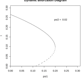
psi2 = 0.02

FIGURE 5.1: A bifurcation diagram for the extended CG model exhibiting backward bifurcation.

Programmes were written in R (2004) to plot dynamic bifurcation diagrams for which

1

ψ was the bifurcation parameter and ψ2 the dynamic parameter. A point on a section of solid curve corresponds to a LAS endemic equilibrium while a point in a dashed section represents an unstable endemic equilibrium. Sets of parameter values were found that produced bifurcation diagrams exhibiting either backward bifurcation or forward bifurcation along with multiple subcritical and supercritical endemic equilibria. Figures 5.1, 5.2 and 5.3 give a sequence of snapshots taken from a dynamic bifurcation diagram. The set of parameter values given by

0 . 4

=

α , µ =0.08,β1 =2.5, β2 =5.3, β3 =6.0, γ1 =0.06 and γ2 =0.04

[image:12.595.161.424.189.441.2]

(13)

0.00 0.05 0.10 0.15 0.20 0.25 0.30

0

.0

0

.0

5

0

.1

0

.1

5

0

.2

0

.2

5

0

.3

0

psi1

I

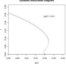
[image:13.595.163.421.74.324.2]

psi2 = 0.14

FIGURE 5.2: A bifurcation diagram for the extended CG model exhibiting forward bifurcation accompanied by two subcritical and three supercritical endemic equilibria.

0.00 0.05 0.10 0.15 0.20 0.25 0.30

0

.0

0

.0

5

0

.1

0

.1

5

0

.2

0

.2

5

0

.3

0

psi1

I

[image:13.595.164.423.418.670.2]

psi2 = 0.2

(14)

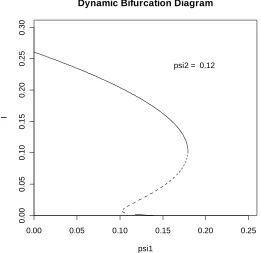
The type of bifurcation curve as given in Figure 5.1 can also be observed for the basic CG model. On the other hand, curves with more complicated shapes, as shown in Figures 5.2 and 5.3, cannot be observed for the simpler version of the model. Of particular interest to us is the fact that these correspond to some of the bifurcation diagrams found for the three-stage BRSV model.

One of the necessary conditions Hadeler and Castillo-Chavez gave for backward bifurcation to occur for the basic CG model was that R~ should be far from 0, remembering that it is also assumed that R~<1. This corresponds to a poor education programme, and equates to

β~ not being too small compared to β . On considering the sets of parameter values used for the bifurcation diagrams in Figures 5.1, 5.2 and 5.3 it would appear that we have a similar, if slightly more complicated, situation for the extended CG model. In order for multiple equilibria (rather than simply backward bifurcation) to be present it seems as though neither of β1 or β2 can be too small compared to β3. In other words, it might be conjectured that for multiple equilibria to be at all possible in the extended CG model, whether via forward or backward bifurcation, neither of the education programmes or methods must be too effective. It is also worth noting that the death rate must not be too large for such curves to be possible here.

5.1 Stability patterns

0.00 0.05 0.10 0.15 0.20 0.25

0

.0

0

.0

5

0

.1

0

.1

5

0

.2

0

.2

5

0

.3

0

psi1

I

[image:14.595.161.422.434.687.2]

psi2 = 0.12

(15)

Now it has been established that complex bifurcation diagrams of the type observed for the three-stage BRSV model are also possible for the extended CG model, we turn our attention to the issue of stability. On the limited evidence of the diagrams given in Figures 5.1, 5.2 and 5.3 it might be conjectured that a particular endemic equilibrium is LAS if, and only if, the gradient at the point on the bifurcation curve corresponding to this equilibrium is negative. However, not only would such a conjecture for the extended CG model be false, but we also observed patterns that we had not seen in any of the literature on backward bifurcation. Before considering this latter phenomenon we give an example to show that stability is not related to the gradient of the bifurcation curve in the simple way that it was for the basic CG model. The diagram in Figure 5.4 was obtained using the following parameter values:

0 . 4

=

α , µ =0.016,β1 =2.5, β2 =5.5, β3 =6.0, γ1 =0.07 and γ2 =0.04.

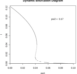
We now demonstrate an interesting stability pattern arising from the extended CG model. The two-stage BRSV and basic CG models have the property that for any particular set of parameter values corresponding to R0 >1 there exists a unique LAS endemic equilibrium. By extending the two-stage BRSV model to three stages we found that it was possible for multiple supercritical endemic equilibria to exist. Furthermore, when multiple supercritical endemic equilibria are present it is quite possible that one of them is unstable. However, for all of the examples that were considered for the three-stage BRSV model it was found that at least one of the resulting supercritical equilibria is LAS. In particular, when there is a unique supercritical endemic equilibrium, it is LAS. On extending the CG model we find that this is not necessarily the case. The bifurcation diagram given in Figure 5.5 was obtained using the following set of parameter values:

5 . 4

=

α , µ=0.01,β1 =2.5, β2 =5.5, β3 =6.0, γ1 =0.11 and γ2 =0.04.

(16)

0.00 0.02 0.04 0.06 0.08 0.10 0 .0 0 0 .0 2 0 .0 4 0 .0 6 0 .0 8 0 .1 0 0 .1 2

psi1

I

psi2 = 0.17

FIGURE 5.5: This bifurcation diagram demonstrates the existence of a unique and unstable supercritical endemic equilibrium for regions in the parameter space.

We emphasise here that the phenomenon observed in Figure 5.5 is not as a result of a lack of sensitivity in the plotting routine. In order to demonstrate this fact we now perform a precise numerical calculation with ψ1 =0.05 in order to check numerically the stability result implied by the bifurcation curve in Figure 5.5. On linearising the system of equations about the endemic equilibrium solution (Se,Ee1,Ee2,Ie) we obtain the Jacobian

              − − + + + − − − + − − − − − + − − − − − µ α β β β β β β αγ β µ β ψ αγ β µ β ψ γ γ α β µ ψ ψ β 2 2 1 1 3 2 1 3 2 2 2 2 2 1 1 1 1 1 2 1 3 2 1 3 0 0 ) 1 ( 0 0 e e e e e e e e e e e e E E S I I I E I E I S I .

[image:16.595.161.422.74.324.2]

(17)

From the fourth equilibrium equation we have β3Se+β1Ee1+β2Ee2 −α−µ =0, so that entry )

3 , 3

( of this matrix can be simplified considerably:

µ α β β β β µ α β β

β3Se+ 1Ee1+ 2(1−Se−Ee1−2Ie)− − = 3Se + 1Ee1+ 2Ee2 − 2Ie− −

e I 2 β − = .

The characteristic equation is thus given by

0 ) ( ) ( ) 1 ( 0 det 2 2 1 2 3 1 1 1 1 1 2 1 3 2 1 3 =           − − − − + − − − − − − + − − − − − − λ β β β β β αγ β λ µ β ψ γ γ α β λ µ ψ ψ β e e e e e e e I I I E I S I .

At this point we note that a study of the local asymptotic stability of the endemic equilibria could, in theory, be performed by analysing the coefficients of the resultant cubic equation in λ via the Routh-Hurwitz criteria. However, we already know that no straightforward stability result will be forthcoming, and so this is not pursued here.

The bifurcation parameter ψ1 was set at 0.05, giving R0 =1.079726.... With the given parameter values the unique endemic equilibrium is calculated to be

...) 003387 . 0 ..., 565830 . 0 ..., 339074 . 0 ..., 091709 . 0 ( ) , , ,

(S_e E_e₁ E_e₂ I_e = .

These equilibrium values have been written as 0.091709..., and so on, to emphasise the fact that all calculations were performed to the highest possible degree of accuracy in order to avoid coming to false conclusions through the accumulation of rounding errors. When substituting these into the characteristic equation we find that two of the eigenvalues have a real part approximately equal to 0.00348, showing that this endemic equilibrium is indeed unstable. This instability does occur at very low levels of infection, and over a relatively narrow range of values of the bifurcation parameter (and, as a consequence, over a particularly narrow range of values of R ). This phenomenon is investigated further in the following section. 0

Before moving on to consider the situation from a stochastic point of view, we note that

the work considered in the current section poses some interesting questions with regard to

dynamic phenomena. Indeed, these might be worth pursuing in a subsequent paper. The

Principle of Exchange of Stability (see Boldin (2006), for example) is certainly relevant here.

This is valid when one stationary state loses its stability to another stationary state in a smooth

way. At a saddle-point bifurcation (also known as a tangential bifurcation or turning point

bifurcation) one of the eigenvalues is zero, and in this case the stability of the branches

representing the various endemic equilibria will depend on the value of the other eigenvalues at

(18)

nongeneric case of a vertical bifurcation and unfold it with two parameters (see van den Bosch

et al. (1988) and Kuznetsov (2004) once more). The dimension of the state space also needs to

be taken into account since Hopf bifurcation may occur when this dimension is at least two.

Indeed, it may be the case that Hopf bifurcation is present in Figure 5.5.

6 Probability of extinction for the basic CG model

We now calculate, for the stochastic version of the basic CG model, the theoretical probability of extinction, given that one infected individual is introduced into the population at the DFE. Before proceeding with the calculation, it is worth pointing out that in general the probability of

extinction does depend on the initial conditions. If, for example, the initial number of infected

individuals was greater than one then we would expect the corresponding probability of

extinction to be reduced. Should R0 be large then the introduction of even one infected

individual into the population could lead to a huge outbreak of the disease in the population. If

the spread of the disease was particularly rapid then this might give rise to a bottle neck in the

supply of susceptible individuals, which may in turn cause the pathogen to go extinct. Since we

are only considering here values of R0 close to one, the possibility of ‘extinction after the first

outbreak’ is not particularly relevant here, although an account of this phenomenon can be

found in Taxidis (2008).

At the DFE the state of the system is given by

   

 

+ +

= , ,0

) , , (

ψ µψ ψ µµ

DFE DFE

DFE V I

S .

Let us consider the discrete branching process

( )

Xˆ_k consisting of the kth generation size of the continuous branching process

( )

I(t) , given that Xˆ0 =I(0)=1. The size of the first generation,

1 ˆ

X , is the total number of individuals that have been directly infected by the initially infected

individual, then X gives the total number of individuals that have been directly infected by the ˆ2

1 ˆ

X individuals in the first generation, and so on. We note that I(t)=0 for some time t if, and only if, Xˆk =0 for some generation k, and so the processes

( )

I(t) and

( )

Xˆk share the same extinction probabilities (see Grimmett and Stirzaker (2001), p. 177).

We next formulate the probability generating function for

( )

Xˆk . Let

µ α ψ µβψ ψ µβµ µ α β

β + +

+ + + = + + +

=

(19)

It shall be assumed that the length of time that an infected individual remains infectious follows a negative exponential distribution with mean 1 (α +µ). Let N be the random variable representing the number of individuals directly infected by one infected individual through its period of infectiousness. It is clear that P(N =0)=(α +µ) ∆. We also have

∆ + × ∆ + − ∆ =

=1) (α µ) α µ

(N

P .

Continuing in this way

n n N P       ∆ + − ∆ ∆ + = = ) ( )

( α µ α µ ,

from which it follows that the probability generating function of the number of individuals infected by one infected individual:

1 0 ) ( 1 ) ( ) ( ) ( − ∞ =            ∆ + − ∆ − ∆ + =             ∆ + − ∆ ∆ + =

=E x

∑

x x

x G

n

N α µ α µ α µ α µ

.

The probability of extinction, P(∞), is given by the smallest positive solution to x=G(x). Solving the equation

1 ) ( 1 −             ∆ + − ∆ − ∆ + = x

x α µ α µ

gives

1

=

x or

0 1 ~ ) )( ( ) ( R x = + + + = + − ∆ + = ψ β βµ µ ψ µ α µ α µ α _.

Thus extinction is certain unless R₀ >1, in which case P(∞)=1 R₀ .

6.1 Stochastic simulations

(20)

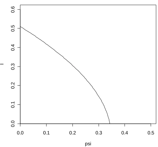
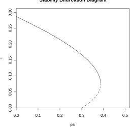
(2004)). Using similar parameter values to those used in the paper by Hadeler and Castillo-Chavez, it is found that forward bifurcation occurs when:

0 . 3

=

α , µ =0.2, β =8.0, β~=0.4 and γ =0.025.

The corresponding bifurcation diagram is given in Figure 6.1.1, noting that the unique supercritical endemic equilibrium is always stable, as given by Theorem 3.1.1 for the basic CG model. We have that ( 0 1) 0.3428...

* = = =

R

ψ

ψ here, as can be seen in Figure 6.1.1.

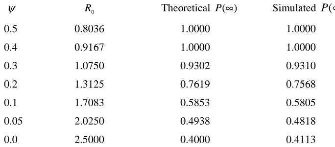
Table 6.1.1 compares, for a range of values of the bifurcation parameter ψ , the theoretical values for P(∞) with those obtained via the simulations. The population size and the number of simulations used to estimate each of these extinction probabilities were 5000 and 4000 respectively. By using a normal approximation to the binomial distribution we may construct approximate confidence intervals from each of the simulated probabilities of extinction in Table 6.1.1 to see if they contain the corresponding theoretical values. For example, an approximate 90% confidence interval for the probability of extinction when

2 . 0

=

ψ is given by [0.7456,0.7680], which does contains the theoretical value. In fact, as is easily checked, all such confidence intervals contain the corresponding theoretical value for

) (∞

P . We see therefore that there is excellent agreement between theoretical and simulated outcomes in this case. It turns out that the simulated values for the probability of extinction do generally match the theoretical values very closely for sets of parameter values leading to forward bifurcation.

0.0 0.1 0.2 0.3 0.4 0.5

0

.0

0

.1

0

.2

0

.3

0

.4

0

.5

0

.6

Stability Bifurcation Diagram

psi

[image:20.595.161.422.484.727.2]

I

(21)

ψ R0 Theoretical P(∞) Simulated P(∞)

0.5 0.8036 1.0000 1.0000

0.4 0.9167 1.0000 1.0000

0.3 1.0750 0.9302 0.9310

0.2 1.3125 0.7619 0.7568

0.1 1.7083 0.5853 0.5805

0.05 2.0250 0.4938 0.4818

0.0 2.5000 0.4000 0.4113

TABLE 6.1.1: A comparison of theoretical and simulated probabilities of extinction for the basic CG model using a set of parameter values leading to forward bifurcation.

It should be noted that increasing the population size from 5000 does not, for the values of ψ used in Table 6.1.1, significantly affect the simulated extinction probabilities. In fact, the population size needs to be reduced considerably for these probabilities to be altered in any way. This is because, as can be seen from Figure 6.1.1, the levels of disease prevalence within the population are relatively high for this particular set of parameter values, even when R is 0 reasonably close to 1. Therefore even fairly small populations will have a relatively large number of infected individuals at quasi-equilibrium, thereby reducing the possibility that a particular random fluctuation will result in extinction.

0.0 0.1 0.2 0.3 0.4

0

.0

0

.1

0

.2

0

.3

0

.4

psi

I

[image:21.595.117.459.56.207.2]

(22)

We now turn our attention to the situation in which backward bifurcation is present. The following set of parameter values lead to the bifurcation diagram given in Figure 6.1.2, noting that the stability pattern is as predicted by Theorem 3.1.1:

0 . 4

=

α , µ =0.1, β =6.0, β~=3.0 and γ =0.02.

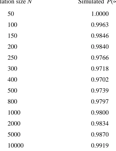
A series of simulations was carried out with ψ =0.18. This gives R0 =0.9930, so the theoretical probability of extinction for this set of parameter values is 1. Table 6.1.2 gives the simulated probability of extinction as the population size N is varied. Each probability of extinction was estimated using 10000 simulations. As well as corroborate the results obtained for the probabilities of extinction for the two-stage BRSV model by Griffiths (2007), our findings offer a fascinating glimpse of the subtle link between deterministic and stochastic phenomena associated with our model.

It is possible to provide heuristic explanations for the interesting relationship observed in Table 6.1.2 between the population size and the probability of extinction estimated via the simulations. As can be seen from the bifurcation curve in Figure 6.1.2, there exists, for

18 . 0

=

ψ , an upper LAS subcritical endemic equilibrium and an unstable lower one. The unstable endemic equilibrium lies on the separatrix for the domains of attraction for the LAS DFE and the LAS endemic equilibrium. It would seem plausible that these deterministic domains of attraction correspond in some way to probabilistic domains of attraction (for the absorbing state I(t)=0 and the quasi-equilibrium respectively) in the stochastic version of the model. The probability of extinction may be related to both the likelihood with which these domains of attraction can be reached and, in cases for which a quasi-equilibrium has been attained, the ability to avoid an extinction due to random fluctuations.

For particularly small population sizes, the low numbers of individuals at quasi-equilibrium make it relatively likely that, over ecologically relevant periods of time (i.e. over several generations), a random fluctuation will result in extinction (since in this case any quasi-equilibrium will be close to the absorbing state). Thus, as when considering the possibility of a supercritical endemic invasion when forward bifurcation is present, we would expect the simulated probability of extinction to tend to 1 as the population size is decreased.

(23)

there is for initial random fluctuations to result in a state lying in this domain of attraction. For very large population sizes this domain of attraction becomes virtually impossible to reach, and extinction is very likely to occur.

From the above discussion it would seem that when backward bifurcation is present, subcritical probabilities of extinction will always tend to 1 as the population becomes either extremely large or extremely small. It is the intermediate population sizes that are of more interest. In these cases the population is still sufficiently small for there to be a realistic prospect of a quasi-equilibrium being attained, while not so small that this quasi-equilibrium is not sustainable over ecologically relevant periods of time.

Population size N Simulated P(∞)

50 1.0000

100 0.9963

150 0.9846

200 0.9840

250 0.9766

300 0.9718

400 0.9702

500 0.9739

800 0.9797

1000 0.9800

2000 0.9834

5000 0.9870

10000 0.9919

TABLE 6.1.2: An illustration of how, for a set of parameter values allowing subcritical endemic equilibria to exist, the estimated probability of extinction varies with the population size.

Population size N 90% confidence interval 99% confidence interval

300 [0.9691, 0.9745] [0.9675, 0.9761]

400 [0.9674, 0.9730] [0.9658, 0.9746]

500 [0.9713, 0.9765] [0.9698, 0.9780]

800 [0.9774, 0.9820] [0.9761, 0.9833]

[image:23.595.180.380.251.512.2]

1000 [0.9777, 0.9823] [0.9764, 0.9836]

(24)

We may calculate confidence intervals for the simulated values of P(∞) shown in Table 6.1.2 in order to add further weight to our argument. Table 6.1.3 provides, for some of the intermediate population sizes, both 90% and 99% confidence intervals for these probabilities. The results in Table 6.1.2 seem to indicate the existence of an ‘optimal’ population size for which the probability of extinction is least. This will be some function of the parameter values and consequently of the level of the disease in the population at quasi-equilibrium. For our particular example the prevalence of the disease at the subcritical LAS endemic equilibrium corresponding to ψ =0.18 is quite high so the disease can be sustained in a relatively small population. For a situation in which the proportion of infected individuals is at a lower level at endemic equilibrium it is likely that this optimal population size will be greater.

7 Probability of extinction for the extended CG model

Further programmes were developed to allow stochastic simulations of the extended CG model. Of particular interest here is the probability of extinction for the case in which there is a unique but unstable supercritical endemic equilibrium in the deterministic version of the model. For

1 0 >

R the theoretical probability of extinction for the stochastic version of the extended CG model is given by

3 2 2 1 1

2

1 )

)( ( ) (

µβ β ψ β

ψ µ ψ ψ µ

α

+ +

+ + +

= ∞

P .

The calculation is similar to that for the probability of extinction for the basic CG model, noting that now ∆=β1EDFE1 +β2EDFE2 +β3SDFE +α +µ. By considering Figure 5.5 it can be seen that the parameter values

05 . 0 1 =

ψ , ψ2 =0.17, α =4.5, µ =0.01,β1 =2.5, β2 =5.5 β3 =6.0, γ1 =0.11 and 04

. 0 2 =

γ

do in fact lead to a unique but unstable supercritical endemic equilibrium. For this set of parameter values P(∞)=0.9262.

The stochastic simulations were initialised by introducing one infected individual into the population at the DFE, given by

   

 

+ + +

+ +

+

= , , ,0

) , , , (

2 1

2 2

1 1 2

1 2

1 ψ ψ µ

ψ µ ψ

ψ ψ

µ ψ

ψ µ

DFE DFE DFE

DFE E E I

(25)

Population sizes ranging from one hundred to one hundred thousand were used. The presence of the absorbing state I =0 in conjunction finite and approximately constant population sizes means that the stochastic model cannot possess a true endemic stationary distribution. However, when the parameter values are such that a deterministic LAS endemic equilibrium exists, the stochastic versions of both the basic and extended CG models do frequently appear to settle down into some sort of steady-state behaviour, resulting in what we have previously termed quasi-equilibria. In these cases it was found that the disease is able to persist within the population for extremely long time periods. Furthermore, these quasi-equilibria tend to match the LAS endemic equilibrium very well indeed. This relationship between the deterministic and stochastic versions of the CG models was also observed when studying the corresponding versions of the BRSV models.

We may clarify this quasi-equilibrium phenomenon by way of an example. A series of simulations of the stochastic version of the basic CG model was performed using the following parameter values (those leading to the bifurcation diagram shown in Figure 6.1.1):

0 . 3

=

α , µ =0.2, β =8.0, β~=0.4 and γ =0.025,

with the bifurcation parameter ψ set at 0.3. As can be seen in Figure 6.1.1, there is a unique deterministic supercritical endemic equilibrium for this set of parameter values, and the proportion of infected individuals at this equilibrium is approximately 10%. The simulations were initialised by introducing one infected individual into a population of 1000 individuals at the DFE. On simulations for which extinction did not occur we saw evidence for the existence of a quasi-equilibrium for which the average number of infected individuals over time is approximately 100, or 10% of the population, demonstrating a quantitative matching with the deterministic endemic equilibrium. Despite the relatively small number of infected individuals, it was found that once the system had reached this quasi-equilibrium then random fluctuations tended not to lead to extinction over the considerable run times of our simulations, thereby implying the presence of a quasi-stationary distribution. There were occasions when a random fluctuation resulted in extinction from an apparent quasi-equilibrium, but these proved to be extremely rare occurrences, and such events became even scarcer as the population size was increased. It would appear that an infected state is acting as a weak attractor in a probabilistic sense.

(26)

infected individual into a population of 10000 individuals at the DFE. A larger population size was used here than since the proportion of infected individuals at the deterministic endemic equilibrium is relatively small, and we do require the absolute number of infected individuals in the population corresponding to this endemic equilibrium to be large enough to determine whether or not there is any evidence of quasi-equilibrium behaviour.

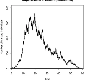
The outcomes of our simulations are potentially very interesting. With a population size of 10000, there are approximately 34 infected individuals at the unstable deterministic endemic equilibrium. However, in none of our simulations did we observe any quasi-equilibrium behaviour for which the average number of infected individuals was approximately this number. On the other hand, potential quasi-equilibrium behaviour was observed for which the average number of infected individuals was considerably greater than 34, typically of the order of 500 individuals. We found either that extinction occurred almost immediately or the number of infected individuals built up over time to several hundred. We may, on the basis of these observations, ponder over the mechanism driving this apparent quasi-equilibrium and then consider whether or not there is a quasi-stationary distribution present. In what follows we may merely speculate on the answers to these questions, and provide some heuristic explanations. Indeed, a more detailed analysis could prove to be extremely difficult.

0 10 20 30 40 50 60

0

2

0

4

0

6

0

8

0

Supercritical invasion (stochastic)

Time

N

u

m

b

e

r

o

f

in

fe

c

te

d

i

n

d

iv

id

u

a

[image:26.595.143.438.402.684.2]

ls

(27)

We considered those realisations for which extinction did not occur in the very early stages of the run. Similar initial behaviour was observed for each of these realisations, with invasions resulting in up to 700 infected individuals being present in the population. In these situations it was almost always the case that, once the number of infected individuals had peaked, a decline occurred, eventually resulting in extinction. An example of such a realisation is shown in Figure 7.1. There were also isolated examples of the disease persisting at these higher levels for slightly longer periods of time. However, even in these instances, it would seem that the system does not remain at the quasi-equilibrium for long enough to indicate the presence of a quasi-stationary distribution.

(28)

determined by the behaviour of the epidemic in the initial stages of an invasion and it is generally possible to obtain a very close match between the simulated and analytic extinction probabilities, even by using relatively short run times in the simulations. In fact, so long as the run times were not too short, we found that our simulations gave estimates that were quite close to the theoretical value 0.9262 obtained from the parameter values given at the beginning of this section. This was also true when obtaining estimates for the probability of extinction for the basic CG model with parameter values as given earlier. In this case estimates close to the analytic extinction probability of 0.9302 resulted from even quite short run times.

On the other hand, from the definition of the probability of extinction, we might expect to obtain ever better agreement between the simulated and theoretical extinction probabilities by extending the run times of our simulations. However, we also know that for finite and approximately constant population sizes, as in our simulations, extinction is bound to occur eventually. It is at this point that we need to take account of whether or not an apparent quasi-equilibrium is able to persist for ecologically relevant periods of time. When a quasi-stationary distribution is present, then, so long as the population size (and hence the number of infected individuals at quasi-equilibrium) is not too small, we may increase the run times considerably in order to obtain more accurate estimates for the theoretical probability of extinction. However, the presence of phenomena such as limit cycles in the deterministic model might mean that increasing the run time gives considerably more opportunities for random fluctuations to result in extinction, and in this case simulated probabilities of extinction are bound to show a corresponding increase. This latter scenario does appear to be the case for the particular set of parameter values we are currently considering for the extended CG model. Simulations do indeed bear this out, with the simulated probability of extinction tending to 1 as the run times increase. Thus the degree to which the simulated and theoretical extinction probabilities agree can, in such situations, be very sensitive with regard to the run times.

This would appear to be a difficult problem to resolve completely, and indeed it may be

worth considering alternative approaches such as those adopted by Kuske et al. (2008) or Allen

and van den Driessche (2006). For example, in the latter paper the authors utilise a stochastic

differential equation model, noting that their deterministic and stochastic models agree very

well when N≥1000. There is also the possibility that R0 may depend on N in some way. Indeed, Nasell (2002) notes that, with regard to the stochastic version of the model he is

studying, there are three identifiable regions of the parameter space with qualitatively different

behaviours, and the boundaries between these regions are dependent on N. He also

(29)

8 Expected time to extinction for the basic CG model

For the two-stage BRSV model Griffiths (2007) found some interesting results in this regard, although, because of the analytic complications, it was not possible to state any definitive results. However, the current situation is more promising since we are able to obtain a precise analytic result for the expected time to extinction given that one infected individual enters the population at the DFE. Note that this is in contrast to the approach adopted by Nasell (2002), who calculates the time to extinction from the quasi-stationary distribution.

Let T be the random variable representing the time to extinction given that one infected individual is introduced into the population at the DFE. Then, using a result from Karlin and Taylor (1975, pp. 149-150), it follows that

        + − + + + + + + =         − + + + + = +

+ _α _µ _µ _ψ _βµ _β_ψ

ψ µ µ α ψ β βµ ψ µ µ α µ α ψ β βµ ψ µ ψ µ βψ

βµ ₍ ₎₍ ₎ ~

) )( ( ln ~ ln ~ ) (

ET ~ .

This may also be written as

      − + = 0 0 1 1 ln ) ( 1 ) ( E R R T µ α ,

which is not defined for R0 ≥1, in which case we write E T( )=∞. We are thus interested in only the subcritical case here. In particular we consider whether the presence of subcritical endemic equilibria exert an influence on E T to the extent that significant differences between ( ) the theoretical and simulated values are observed.

We first demonstrate that our programmes are working correctly in the sense that they lead to simulated estimates for E T that are in good agreement with the corresponding analytic ( ) values under what we may regard as ‘ideal’ conditions. We start therefore with the following set of parameter values leading to forward bifurcation:

0 . 3

=

α , µ =0.2, β =8.0, β~=0.4 and γ =0.025.

(30)

ψ R0 Theoretical E T ( ) Simulated E T ( )

0.5 0.8036 0.6329 0.6284, 0.6483, 0.6294, 0.6301

0.75 0.6250 0.4904 0.4900, 0.4879, 0.4921, 0.4864

1.0 0.5208 0.4414 0.4361, 0.4542, 0.4431, 0.4544

TABLE 8.1: A comparison of theoretical and simulated expected times to extinction for the basic CG model using a set of parameter values leading to forward bifurcation.

We next run simulations for the system with parameter values given by:

0 . 4

=

α , µ =0.2, β =6.0, β~=3.0 and γ =0.025.

The corresponding bifurcation diagram, exhibiting backward bifurcation, is shown in Figure 8.1.

0.0 0.1 0.2 0.3 0.4 0.5

0

.0

0

.0

5

0

.1

0

.1

5

0

.2

0

.2

5

0

.3

0

psi

[image:30.595.120.444.76.192.2]

I

FIGURE 8.1: A bifurcation diagram for the basic CG model exhibiting backward bifurcation.

[image:30.595.163.423.389.639.2]

(31)

{

}

_   

  

− + − − − + − −

= (1 )( ~) ~ ( ~)

~ ~

1

# α γ α µ β µβ α µ β

ββ β β

e I

although the estimate of ( #)≈0.4

e

I

ψ from the bifurcation diagram will certainly suffice for present purposes.

We compare theoretical and analytic values for E T using various values of ( ) ψ greater than ψ(Ie#). In particular, we are interested in determining whether or not there is any evidence that the deterministic LAS subcritical endemic equilibrium present when ψ is slightly smaller than ψ(Ie#) is able to influence the stochastic behaviour of the system for slightly larger values of ψ (for which no deterministic endemic equilibria are present). Indeed, if this were the case, and an ecologically unstable quasi-equilibria occasionally resulted when ψ was just above

) ( #

e

I

ψ , then we might expect the simulated values of E T to be significantly greater than the ( ) corresponding analytic values. The results of the simulations, using the parameter values leading to the bifurcation diagram in Figure 8.1, are given in Table 8.2. The conditions for each simulation were the same as those used to obtain the results in Table 8.1.

ψ R0 Theoretical E T ( ) Simulated E T ( )

0.42 0.9447 0.7296 0.7664, 0.7680, 0.7515, 0.7704

0.44 0.9375 0.7041 0.7534, 0.7366, 0.7113, 0.7241

0.6 0.8929 0.5956 0.6168, 0.5862, 0.6082, 0.6140

1.0 0.8333 0.5119 0.5116, 0.5119, 0.5063, 0.5174

TABLE 8.2: A comparison of theoretical and simulated expected times to extinction for the basic CG model using a set of parameter values leading to backward bifurcation.

In Table 8.2, it may be seen that values of ψ just above ( #)

e

I

ψ tend to lead to the simulations giving significant overestimates for the theoretical values of E T , but as we ( ) increase ψ there is ever better agreement between the simulated and theoretical values. We feel that these results, though not totally conclusive, do lend weight to our argument concerning the possibility that ecologically unstable quasi-equilibria are present for values of ψ just above

) ( #

e

I

(32)

individual runs, that the overestimates mentioned above, when ψ was just above ψ(Ie#), tended to be caused by a very small proportion of relatively long-lived, but still ecologically unstable, quasi-equilibria.

9 More unusual bifurcation diagrams

We have thus far only analysed the system consisting of an isolated core population of constant size. It is now time to consider the population as a whole. We expand on some of the interesting ideas that were briefly considered by Hadeler and Castillo-Chavez towards the end of their paper. We make the point here that much of the content of this particular section is not new. However, due to the brevity of the discussion in the original paper we feel that these ideas do deserve to be explained in a little more detail, and ought also to be considered within the context of the extended CG model.

The basic CG model arose from the following more general model:

A C I Ar P dt

dA _µ _µ

− −

= ( , ) (9.1)

S I S

C SI C

I Ar dt

dS _β _ψ _α _γ _µ

− − + − −

= ( , ) (1 ) , (9.2)

V I C VI S dt

dV _ψ _β _αγ _µ

− + −

= ~ (9.3)

and I I

C VI SI dt

dI ₌ β +β~ ₋_α ₋_µ

, (9.4)

where the total population size P is constant but the core group size C is not, in general, constant. We have that P= A+C= A+S+V +I where A is the sexually inactive non-core group. The function r( CI, ) describes the rate of recruitment into the core group from the non-core group. We may, once more, look for endemic equilibria by setting the time derivatives to zero. If (Ae,Se,Ve,Ie) is an endemic equilibrium of the above system then

e e

e S V I P A

C = + + = − . Equation (9.1) gives µ(P−Ae)−Aer(Ie,Ce)=0, from which we see that Aer(Ie,Ce)=µCe. On substituting this into (9.2) we obtain the following set of equilibrium equations:

0 )

1

( − − =

+ −

− e e e

e e e

e S I S

C I S

C β ψ α γ µ

µ ,

0

~ ₊ ₋ ₌

− e e

e e e

e I V

C I V

S β αγ µ