Approximation Methods for Hybrid Diffusion Systems
with State-dependent Switching Processes: Numerical
Algorithms and Existence and Uniqueness of Solutions
G. Yin,
∗Xuerong Mao,
†Chenggui Yuan,
‡Dingzhou Cao
§Abstract
By focusing on hybrid diffusions in which continuous dynamics and discrete events coexist, this work is concerned with approximation of solutions for hybrid stochastic differential equations with a state-dependent switching process. Iterative algorithms are developed. The continuous-state dependent switching process presents added dif-ficulties in analyzing the numerical procedures. Weak convergence of the algorithms is established by a martingale problem formulation first. This weak convergence result is then used as a bridge to obtain strong convergence. In this process, the existence and uniqueness of the solution of the switching diffusions with continuous-state-dependent switching are obtained. Different from the existing results of solutions of stochastic dif-ferential equations in which the Picard iterations are utilized, Euler’s numerical schemes are considered here. Moreover, decreasing stepsize algorithms together with their weak convergence are given. Numerical experiments are also provided for demonstration.
Key Words. Switching diffusion, numerical algorithm, convergence, existence and uniqueness of strong solution.
AMS Subject Classification. 65C30, 60H35, 65C05.
Running Title. Approximation of Switching Diffusions
∗Department of Mathematics, Wayne State University, Detroit, U.S.A. The research of this author was supported in part by the National Science Foundation.
†Department of Statistics and Modelling Science, University of Strathclyde, Glasgow G1 1XH, U.K. ‡Department of Mathematics, University of Wales Swansea, Swansea SA2 8PP, U.K.
1
Introduction
Recently, hybrid systems in which continuous dynamics and discrete events coexist have drawn much attention. In particular, resurgent efforts have been devoted to the research on switching diffusion systems (also known as regime-switching diffusions). Much of the study was originated from applications arising from two-time-scale systems, control engineering practice, manufacturing systems, estimation and filtering, and financial engineering; see [5, 7, 15, 17, 19, 20, 21, 24], among others. Recent progress for switching diffusions has been summarized in [14] and references therein. Up to this point, the study has been carried out for such systems whose switching component is a continuous-time Markov chain independent of the continuous state variable [13, 23], whereas lesser is known for the processes with continuous-state-dependent switching [1, 25]. Nevertheless, in many applications, discrete events and continuous dynamics are intertwined, and the independence assumption of the discrete-event process and the continuous component poses restrictions. It would be nice to be able to handle the coupling and dependence of the continuous states and discrete events. Numerical methods for stochastic differential equations have been studied extensively, for example in [4, 9, 16] among others, whereas numerical solutions for stochastic differential equations with Markovian switching have also been well studied (see [14] and the many references therein). Numerical solutions with state-dependent switching diffusions have not been well understood to the best of our knowledge.
Suppose that M={1, . . . , m} is a finite set. Consider the hybrid diffusion system
dx(t) =f(x(t), α(t))dt+σ(x(t), α(t))dw(t),
x(0) = x0, α(0) =α0,
(1.1)
and
P(α(t+ ∆t) =j|α(t) = i, x(s), α(s), s≤t) =qij(x(t))∆t+o(∆t), i6=j, (1.2)
wherew(·) is anr-dimensional standard Brownian motion,x(t)∈Rr,f(·,·) :Rr× M 7→Rr,
andσ(·,·) :Rr×M 7→Rr×rare appropriate functions satisfying certain regularity conditions, and Q(x) = (qij(x))∈ Rm×m satisfies that for each x, qij(x) ≥ 0 for i 6=j, Pmj=1qij(x) = 0 for eachi∈ M. There is an associated operator for the switching diffusion process defined as follows. Use z′ to denote the transpose ofz, and use ∇ and ∇2 as the notation for gradient
operator
Lh(x, i) =∇h′(x, i)f(x, i) + 1 2tr[∇
2h(x, i)σ(x, i)σ′(x, i)] +
m
X
j=1
qij(x)h(x, j). (1.3)
The state-dependent model is largely motivated by applications in control and optimiza-tion. Similar to the literature in Markov decision processes, we may consider a Markov process (x(t), α(t)) whose generator has control dependence and the control is in feedback form resulting in the consideration of switching process being state dependent. The consid-eration of M being a finite set is mainly from an application point of view. For emerging applications arising in manufacturing, wireless communication, and finance, the set M is naturally a finite set. In principle, Mcan be an infinite set. However, ifMis an infinite set, we will need to deal with a coupled system with infinitely many components. In numerical approximation, we shall approximate the resulting system with finitely many components. For suchM, we often approximate it by a large-dimensional finite setM. Reduction of com-putational complexity for large-scale systems can be carried out using a time-scale separation approach [22].
Since the solution of (1.1) can often be obtained only through numerical approximations, constructing numerical solutions is of foremost importance. In this paper, our aim is to construct numerical approximation schemes for solving (1.1) withα(t) taking values inM=
{1, . . . , m}. The novelty of our work lies in thatQ(x), the generator of the switching process
α(t), is state dependent, which makes the analysis much more difficult. One of the main difficulties is that due to the continuous-state dependence, α(t) and x(t) are dependent;
α(t) is a Markov chain only for a fixed x but is otherwise non-Markovian. Unlike the usual diffusion processes represented by stochastic differential equations, the distribution of the switching diffusion has mixture distribution. The essence in our approach is to treat the pair of processes (x(t), α(t)) jointly; the two-component process turns out to be Markovian. Nevertheless, much care needs to be exercised to handle the mixture distributions. To proceed, we will use the following conditions.
(A1) TheQ(·) :Rr7→Rm×m is a bounded and continuous function.
(A2) The functions f(·,·) andσ(·,·) satisfy
(a) |f(x, α)| ≤K(1 +|x|),|σ(x, α)| ≤K(1 +|x|), and
(b) |f(x, α)−f(z, α)| ≤K0|x−z| and|σ(x, α)−σ(z, α)| ≤K0|x−z|for some K >0
Note that condition (A1) is simply a condition on the function Q(x). If Q(x) = Q, we are back to the case of Markovian switching diffusions. Here owing to the x-dependence, the problem becomes more complex. The switching process and the diffusions are intertwined and dependent. Using Poisson random measures (see [18] and also [1]), under conditions (A1) and (A2), it can be shown that (1.1) has a unique solution for each initial condition by following Ikeda and Watanable [6] with the appropriate use of the stopping times. However, the Picard iteration method does not work. In this paper, we construct Euler’s scheme with a constant stepsize for approximating solutions of switching diffusions. As a result, our method differs from the usual approach. To obtain the convergence of the algorithms, we first show the weak convergence of the algorithm by means of martingale problem formulation. Then this result is used as a bridge to obtain strong convergence. In this process, we prove the existence and uniqueness of the solution of (1.1). This result is of independent interest in its own right; it enables us to obtain the strong convergence of the numerical algorithms. As a demonstration, we provide numerical experiments to delineate sample path properties of the approximating solutions. In addition, we present a decreasing stepsize algorithm, and obtain its weak convergence.
To see that the state-dependence switching can contribute to much of the difficulty, we consider the following scenario. Let a switching diffusion (x(t), α(t)) be given by (1.1). First let the initial data be (x(0), α(0)) = (x, α) and then consider another initial data (x(0), α(0)) = (y, α) fory 6=x. For the state-dependent switching case, since Q(x) depends onx,αx,α(t)6=αy,α(t) infinitely often even though initiallyαx,α(0) =αy.α(0) =α, where the superscript above denotes the initial data dependence.
In what follows, for notational simplicity, we use the convention that K represents a generic positive constant, whose values may be different for different appearances so that
K+K =K andKK =K is understood in an appropriate sense. In addition, forz ∈Rι1×ι2
for some ιi ≥1, z′ denotes the transpose ofz.
to the solution of a martingale problem with a desired generator. Hence the limit is the solution of the system of switching diffusions. Section 4 presents a couple of computational examples. Also provided in this section is a decreasing stepsize algorithm. Section 5 makes a few more remarks to conclude the paper.
2
Numerical Methods
To approximate the r-dimensional standard Brownian motion w(·), we use a sequence of independent and identically distributed Gaussian random variables {ξn} for simplicity. To approximate the solution of (1.1), we propose the following algorithm
xn+1 =xn+εf(xn, αn) +√εσ(xn, αn)ξn. (2.1) We would like to have αn be a discrete-time stochastic process that approximates α(t) in an appropriate sense. It is natural that αn has a transition probability matrix exp(Q(x)ε) when xn−1 = x. It is easily seen that the transition matrix may be approximated further
by I +εQ(x) +O(ε2) by virtue of the boundedness and the continuity of Q(·). Based on
this observation, in what follows, we discard the O(ε2) term and simply use I +εQ(x) for the transition matrix for αn when xn−1 =x. We put what we said above into the following
assumption.
(A3) In (2.1), for each n, when xn−1 = x, αn has the transition matrix I +εQ(x), and {ξn} is a sequence of independent and identically distributed random variables with normal distribution such that ξn is independent of the σ-algebra Gn generated by {xk, αk :k ≤n}, and thatEξn = 0 and Eξnξn′ =I.
Remark 2.1. One of the features of (2.1) is that it is easily implementable. In lieu of discretizing a Brownian motion, we generate a sequence of independent and identically dis-tributed random variables with normal distribution to approximate the Brownian motion. This facilitates the computational task. In addition, instead of using transition matrix exp(εQ(x)) for a fixed x, we use another fold of approximation I+εQ(x) based on a trun-cated Taylor series. All of these stem from consideration of numerical computation and Monte Carlo implementation.
3
Convergence of the Algorithm
3.1
Preliminary Estimates
We first obtain an estimate on the pth moment of {xn}. This is stated as follows.
Lemma 3.1. Under (A1), (A2) and (A3), for any fixed p≥2 and T >0,
sup
0≤n≤T /ε
E|xn|p ≤(|x0|p+KT) exp(KT)<∞. (3.1)
Remark 3.2. Throughout this paper, we assume the stepsize 0 < ε < 1. Note that in Lemma 3.1, by T /ε, we mean the integer part of T /ε, i.e., ⌊T /ε⌋. However, for simplicity, we will not use the floor function notation in what follows.
Note that in the proof of Lemma 3.1,U(x) is a Liapunov type function. The technique used is standard in stochastic approximation [11, Chapter 5]. If correlated random sequences are treated, we can use a perturbed Liapunov function technique [11, Section 4.5, p.112].
Proof of Lemma 3.1. DefineU(x) =|x|p and useE
nto denote the conditional expectation
with respect to the σ-algebra Gn, where Gn was given in (A3). Note that Enσ(xn, αn)ξn = σ(xn, αn)Enξn= 0 and thatEn|σ(xn, αn)|2|ξn|2 =|σ(xn, αn)|2En|ξn|2 ≤K|σ(xn, αn)|2,where K is a generic positive constant. Thus
EnU(xn+1)−U(xn) = En∇U′(xn)[xn+1−xn] +En(xn+1−xn)′∇2U(x+n)(xn+1−xn)
≤ε∇U′(xn)f(xn, αn) +K|xn|p−2En|xn+1−xn|2
≤εK|xn|p−1(1 +|xn|) +Kε|xn|p−2(1 +|xn|2) +Kε2|xn|p−2(1 +|xn|2) ≤Kε(1 +|xn|p),
(3.2) where ∇U and ∇2U denotes the gradient and Hessian of U w.r.t. to x, and x+
n denotes a vector on the line segment joining xn and xn+1. Note that in the last line of (3.2), we
have used the linear growth in x for both f(·,·) and σ(·,·). Since U(xn) =|xn|p, we obtain En|xn+1|p ≤ |xn|p +Kε+Kε|xn|p. Taking the expectation on both sides and iterating on the resulting recursion, we obtain
E|xn+1|p ≤ |x0|p+Kεn+Kε
n
X
k=0
E|xk|p.
An application of the Gronwall’s inequality yields thatE|xn+1|p ≤(|x0|p+KT) exp(KT) as
In view of the estimate above, {xn : 0 ≤ n ≤ T /ε} is tight in Rr by means of the well-known Tchebyshev’s inequality. That is, for eachη >0, there is aKηsatisfyingKη >
p
(1/η) such that
P(|xn|> Kη)≤ sup
0≤n≤T /ε
E|xn|2
K2
η
≤Kη.
This indicates that the sequence of iterates is “mass preserving” or no probability is lost. To proceed, take continuous-time interpolations defined by
xε(t) =xn, αε(t) =αn, for t ∈[nε, nε+ε). (3.3)
We shall show that xε(·) andαε(·) are tight in suitable function spaces.
Lemma 3.3. Assume (A1)–(A3). Define
χn= (I{αn=1}, . . . , I{αn=m})∈R
1×m and χε(t) = χ
n, for t∈[εn, εn+ε). (3.4)
Then for any t, s >0,
E[χε(t+s)−χε(t)Ftε] =O(s), (3.5)
where Fε
t denotes the σ-algebra generated by {xε(u), αε(u) :u≤t}.
Proof. First note that by the boundedness and the continuity of Q(·), for each i∈ M, m
X
j=1
E[I{αk+1=j}−I{αk=i}
Gk]
= m
X
j=1
[(I+εQ(xk))ij−δij]I{αk=i}
= m
X
j=1
εqij(xk)I{αk=i} =O(ε)I{αk=i},
where (I+εQ(xk))ij denotes the ijth entry ofI+εQ(xk) and δij =
1, if i=j,
0, otherwise. It then follows that there is a random function eg(·) such
E[
(t+s)/ε−1
X
k=t/ε
[χk+1−χk]
Ftε]
=E[
(t+s)/ε−1
X
k=t/ε
E[χk+1−χk
Gk]
Ftε]
=eg(t+s−t) =eg(s),
and that Eeg(s) = O(s). In the above, we have used the convention that t/ε and (t+s)/ε
denote the integer parts of t/ε and (t+s)/ε, respectively. Since
Ehχε(t+s)−χε(t)−
(t+Xs)/ε−1
k=t/ε
[χk+1−χk]
Ftε
i
= 0,
it follows from (3.6),
E[χε(t+s)
Fε
t] = χε(t) +eg(s). The desired result then follows.
Lemma 3.4. Under the conditions of Lemma 3.3, {αε(·)} is tight.
Proof. For anyη >0, t≥0, 0≤s≤η, by virtue of Lemma 3.3,
E[|χε(t+s)−χε(t)|2Ftε]
=E[χε(t+s)χε,′(t+s)−2χε(t+s)χε,′(t) +χε(t)χε,′(t)
Ftε]
= m
X
i=1
E[I{α(t+s)/ε=i}−2I{α(t+s)/ε=i}I{αt/ε=i}+I{αt/ε=i}
Ftε].
(3.7)
The estimates in Lemma 3.3 then imply that
lim
η→0lim supε→0 E[E|χ
ε(t+s)
−χε(t)|2Ftε] = 0.
The tightness criterion in [10, p. 47] yields that {χε(·)} is tight. Consequently, {αε(·)} is tight.
Lemma 3.5. Assume that the conditions of Lemma 3.4 are satisfied. Then {xε(·)} is tight in Dr[0,∞), the space of functions that are right continuous and have left limits, endowed
Proof. For anyη >0, t≥0, 0≤s≤η, we have
E|xε(t+s)−xε(t)|2 =E
ε
(t+s)/ε−1
X
k=t/ε
f(xk, αk) +√ε
(t+s)/ε−1
X
k=t/ε
σ(xk, αk)ξk
2
≤Kε2
(t+s)/ε−1
X
k=t/ε
(1 +E|xk|2) +Kε
(t+s)/ε−1
X
k=t/ε
E|σ(xk, αk)|2E|ξk|2
≤Kε2
(t+s)/ε−1
X
k=t/ε
(1 + sup
t/ε≤k≤(t+s)/ε−1
E|xk|2)
+Kε
(t+s)/ε−1
X
k=t/ε
(1 + sup
t/ε≤k≤(t+s)/ε−1
E|xk|2)
≤O
t+s ε −
t ε
O(ε) = O(s).
(3.8)
In the above, we have used Lemma 3.1 to ensure that supt/ε≤k≤(t+s)/ε−1E|xk|2 <∞. There-fore, (3.8) leads to
lim
η→0lim supε→0 E|x
ε(t+s)
−xε(t)|2 = 0.
The tightness of {xε(·)}then follows from [10, p. 47].
With Lemma 3.3, Lemma 3.4, and Lemma 3.5 at our hands, we obtain the following result.
Lemma 3.6 Under assumptions (A1)–(A3), {xε(·), αε(·)} is tight in D([0,∞) :Rr× M).
3.2
Weak Convergence
Since (xε(·), αε(·)) is tight, by Prohorov’s theorem (see [3, 11]), we may select a convergent subsequence. For simplicity, still denote the subsequence by (xε(·), αε(·)) with limit denoted by (xe(·),αe(·)).
Theorem 3.7. Assume (A1)–(A3). Then {xε(·), αε(·)} converges weakly to (x(·), α(·)),
which is a process with generator given by (1.3).
Proof. By Skorohod representation (see [3, 11]) without loss of generality and without changing notation, we may assume that (xε(·), αε(·)) converges to (
e
x(·),αe(·)) w.p.1, and the convergence is uniform on each bounded interval. We proceed to characterize the limit process.
Step 1: We first work with the marginal of the switching component, and characterize the limit of αε(·). The weak convergence of αε(·) to
e
process χ(·) weakly, whereχε(·) was defined in (3.4). For each t >0 ands >0, each positive integer κ, each 0≤tι ≤t withι ≤κ, each bounded and continuous functionρ0(·, i) for each
i∈ M,
Eρ0(xε(tι), αε(tι), ι≤κ)
h
χε(t+s)−χε(t)−
(t+s)/ε−1
X
k=t/ε
(χk+1−χk)
i
= 0. (3.9)
The weak convergence of χε(·) to χ(·) and the Skorohod representation imply that
lim
ε→0Eρ0(x
ε(t
ι), αε(tι), ι≤κ)[χε(t+s)−χε(t)] =Eρ0(xe(tι),αe(tι), ι≤κ)[χ(t+s)−χ(t)].
Pick out a sequence {nε} of nonnegative real numbers such that nε → ∞ as ε → 0 but δε =εnε →0.
Let Ξε
l be the set of indices
Ξεl ={k :lnε ≤k≤lnε+nε−1}. (3.10)
Then the continuity and boundedness of Q(·) imply
lim ε→0Eρ0(x
ε(t
ι), αε(tι), ι≤κ)
h(t+s)/ε−1
X
k=t/ε
(χk+1−χk)
i
= lim
ε→0Eρ0(x
ε(t
ι), αε(tι), ι≤κ)
h(t+s)/ε−1
X
k=t/ε
(E(χk+1
Gk)−χk)
i
= lim
ε→0Eρ0(x
ε(t
ι), αε(tι), ι≤κ)
h(t+s)/ε
X
lnε=t/ε
X
k∈Ξε l
χk(I+εQ(xk)−I)
i
= lim
ε→0Eρ0(x
ε(t
ι), αε(tι), ι≤κ)
h(t+s)/ε
X
lnε=t/ε
δε 1
nε
X
k∈Ξε l
χkQ(xlnε)
i
.
(3.11)
Note that
lim ε→0Eρ0(x
ε(t
ι), αε(tι), ι≤κ)
h(tX+s)/ε
lnε=t/ε
δε 1
nε
X
k∈Ξε l
[χk−χlnε]Q(xlnε)
i
= lim
ε→0Eρ0(x
ε(t
ι), αε(tι), ι≤κ)
h(tX+s)/ε
lnε=t/ε
δε 1
nε
X
k∈Ξε l
E[χk−χlnε
Glnε]Q(xlnε)
i
= lim
ε→0Eρ0(x
ε(t
ι), αε(tι), ι≤κ)
h(t+s)/ε
X
lnε=t/ε
δε 1
nε
X
k∈Ξε l
Eχlnε[(I+εQ(xlnε))
k−lnε
−I]Q(xlnε)
i
= 0.
Therefore,
lim
ε→0Eρ0(x
ε(t
ι), αε(tι), ι≤κ)
h(tX+s)/ε
lnε=t/ε
δε 1
nε
X
k∈Ξε l
χkQ(xlnε)
i
= lim
ε→0Eρ0(x
ε(t
ι), αε(tι), ι≤κ)
h(t+s)/ε
X
lnε=t/ε
δεχlnεQ(xlnε)
i
=Eρ0(xe(tι),αe(tι), ι≤κ)
Z t+s
t
χ(u)Q(xe(u))du.
(3.13)
Moreover, the limit does not depend on the chosen subsequence. Thus,
Eρ0(xe(tι),αe(tι), ι≤κ)
h
χ(t+s)−χ(t)−
Z t+s
t
χ(u)Q(xe(u))dui= 0. (3.14)
Therefore, the limit process αe(·) has a generator Q(ex(·)).
Step 2: Fort, s,κ, tι as chosen before, for each bounded and continuous function ρ(·, i), and for each twice continuously differentiable function with compact support h(·, i) with
i∈ M, we shall show that
Eρ(xe(tι),αe(tι);ι ≤κ)[h(xe(t+s),αe(t+s))−h(xe(t),αe(t))−
Z t+s
t L
h(xe(u),αe(u))du] = 0.
(3.15) This yields that
h(ex(t),αe(t))−
Z t
0 L
h(xe(u),αe(u))du is a continuous-time martingale,
which in turn implies that (xe(·),αe(·)) is a solution of the martingale problem with operator
L defined in (1.3).
To establish the desired result, we work with the sequence (xε(·), αε(·)). Again, we use the sequence {nε} as in Step 1. By virtue of the weak convergence and the Skorohod representation, it is readily seen that
Eρ(xε(tι), αε(tι);ι≤κ)[h(xε(t+s), αε(t+s))−h(xε(t), αε(t))]
→Eρ(xe(tι),αe(tι);ι≤κ)[h(xe(t+s),αe(t+s))−h(xe(t),αe(t))] as ε→0.
(3.16)
On the other hand, direct calculation shows that
Eρ(xε(tι), αε(tι);ι≤κ)[h(xε(t+s), αε(t+s))−h(xε(t), αε(t))]
=Eρ(xε(tι), αε(tι);ι≤κ)
n(t+Xs)/ε−1
lnε=t/ε
h
[h(xlnε+nε, αlnε+nε)−h(xlnε+nε, αlnε)]
+[h(xlnε+nε, αlnε)−h(xlnε, αlnε)]
io
.
Step 3: Still use the notation Ξε
ℓ defined in (3.10). For the terms on the last line of (3.17), we have
lim ε→0Eρ(x
ε(t
ι), αε(tι);ι≤κ)
(t+Xs)/ε−1
lnε=t/ε
[h(xlnε+nε, αlnε)−h(xlnε, αlnε)]
= lim ε→0Eρ(x
ε(t
ι), αε(tι);ι≤κ)
n(t+s)/ε−1
X
lnε=t/ε
h
ε∇h′(xlnε, αlnε)
X
k∈Ξε l
f(xk, αlnε)
+ε 2
X
k∈Ξε l
tr[∇2h(xlnε, αlnε)σ(xk, αlnε)σ ′(x
k, αlnε)]
io
.
(3.18) By the continuity off(·, i) for each i∈ M and the choice ofnε,
lim ε→0Eρ(x
ε(t
ι), αε(tι);ι≤κ)
n(t+s)/ε−1
X
lnε=t/ε
δε∇h′(xlnε, αlnε)
1
nε
X
k∈Ξε l
[f(xk, αlnε)−f(xlnε, αlnε)]
o
= 0.
Thus, in evaluating the limit, f(xk, αlnε) can be replaced by f(xlnε, αlnε).
The choice ofnεimplies thatεlnε →uasε→0 yieldingεk →ufor alllnε ≤k≤lnε+nε. Consequently, by the weak convergence and the Skorohod representation,
lim ε→0Eρ(x
ε(t
ι), αε(tι);ι≤κ)
n(t+s)/ε−1
X
lnε=t/ε
ε∇h′(xlnε, αlnε)
X
k∈Ξε l
f(xk, αlnε)
o
= lim ε→0Eρ(x
ε(t
ι), αε(tι);ι ≤κ)
n(t+s)/ε−1
X
lnε=t/ε
δε∇h′(xlnε, αlnε)
1
nε
X
k∈Ξε l
f(xlnε, αlnε)
o
= lim ε→0Eρ(x
ε(t
ι), αε(tι);ι ≤κ)
n(t+s)/ε−1
X
lnε=t/ε
δε∇h′(xlnε, αlnε)f(x
ε(lδ
ε), αε(lδε))
o
=Eρ(ex(tι),αe(tι);ι≤κ)
n Z t+s
t ∇
h′(xe(u),αe(u))f(xe(u),eα(u))duo.
(3.19)
In the above, treating such terms asf(xε(lδ
ε), αε(lδε)), we can approximatexε(·) by a process taking finitely many values using a standard approximation argument (see for example, [11, p. 169] for more details).
Similar to (3.19), we also obtain
lim ε→0Eρ(x
ε(t
ι), αε(tι);ι≤κ)
nε
2
(t+Xs)/ε−1
lnε=t/ε
X
k∈Ξε l
tr[∇2h(xlnε, αlnε)σ(xk, αlnε)σ ′(x
k, αlnε)]
o
=Eρ(ex(tι),αe(tι);ι≤κ)
n Z t+s
t 1 2tr[∇
2h(
e
x(u),αe(u))σ(ex(u),αe(u))σ′(xe(u),αe(u))]duo.
Step 4: We next examine the terms on the next to the last line of (3.17). First, again using the continuity, the weak convergence, and the Skorohod representation, it can be shown that
lim ε→0Eρ(x
ε(t
ι), αε(tι);ι≤κ)
n(t+s)/ε−1
X
lnε=t/ε
[h(xlnε+nε, αlnε+nε)−h(xlnε+nε, αlnε)]
o
= lim ε→0Eρ(x
ε(t
ι), αε(tι);ι≤κ)
n(t+s)/ε−1
X
lnε=t/ε
[h(xlnε, αlnε+nε)−h(xlnε, αlnε)]
o
.
(3.21)
That is, owing to the choice of {nε} and the continuity of h(·, i), the term
h(xlnε+nε, αlnε+nε)−h(xlnε+nε, αlnε)
in the next to the last line of (3.17) can be replaced by
h(xlnε, αlnε+nε)−h(xlnε, αlnε)
as far as asymptotic analysis is concerned. It follows that
lim ε→0Eρ(x
ε(t
ι), αε(tι);ι≤κ)
n(t+s)/ε−1
X
lnε=t/ε
[h(xlnε, αlnε+nε)−h(xlnε, αlnε)]
o
= lim ε→0Eρ(x
ε(t
ι), αε(tι);ι≤κ)
n(t+s)/ε−1
X
lnε=t/ε
X
k∈Ξε l
[h(xlnε, αk+1)−h(xlnε, αk)]
o
= lim ε→0Eρ(x
ε(t
ι), αε(tι);ι≤κ)
n(t+s)/ε−1
X
lnε=t/ε
X
k∈Ξε l
m
X
i=1
m
X
i1=1
Eh[h(xlnε, i)I{αk+1=i}
−h(xlnε, i1)I{αk=i1}]
Gk
io
.
(3.22) Note that for k≥lnε,
E[[h(xlnε, i)I{αk+1=i}−h(xlnε, i1)I{αk=i1}]
Gk] = [h(xlnε, i)P(αk+1 =i
Gk, αk =i1)−h(xlnε, i1)]I{αk=i1}
= [h(xlnε, i)(δi1i+εqi1i(xk))−h(xlnε, i1)]I{αk=i1}
=εh(xlnε, i)qi1i(xk)I{αk=i1}.
(3.23)
Using (3.23) in (3.22) and noting the continuity and boundedness of Q(·), we can replace
by I{αε(εlnε)=i1}, again yielding the same limit. Thus, we have
lim ε→0Eρ(x
ε(t
ι), αε(tι);ι≤κ)
n(t+s)/ε−1
X
lnε=t/ε
[h(xlnε, αlnε+nε)−h(xlnε, αlnε)]
o
=Eρ(xe(tι),αe(tι);ι≤κ)
n Z t+s
t
Q(ex(u))h(xe(u),·)(αe(u))duo,
(3.24)
where
Q(x)h(x,·)(i1) =
m
X
i=1
qi1i(x)h(x, i) =
X
i6=i1
qi1i(x)(h(x, i)−h(x, i1)).
Step 5: Combining Steps 1–4, we arrive at (xe(·),αe(·)), the weak limit of (xε(·), αε(·)) is a solution of the martingale problem with operator L defined in (1.3). Using characteristic functions, we can show as in [22, Lemma 7.18], (x(·), α(·)) the solution of the martingale problem with operator L, is unique in the sense of in distribution. Thus (xε(·), αε(·)) con-verges to (x(·), α(·)) as desired, which concludes the proof of the theorem.
3.3
Existence and Uniqueness of the Solutions
We have established convergence of (xε(·), αε(·)) to (x(·), α(·)) in the weak sense. In this sec-tion, we strengthen the approximation result. We shall show that the weak limit (x(·), α(·)) is, in fact, the strong solution of Eq. (1.1). Define the continuous approximation of xε(t), i.e.,
¯
Xε(t) =x0+
Z t
0
f(xε(s), αε(s))ds+
Z t
0
σ(xε(s), αε(s))dw(s). (3.25)
Note that ¯Xε(εk) =xε(εk) =x
k and αε(εk) =αk. That is, ¯Xε(t) and xε(t) coincide at the gridpoints k =t/ε (again,t/ε means⌊t/ε⌋, the integer part of t/ε).
Theorem 3.8. Assume(A1)–(A3). Then there exists a unique solution to Eq. (1.1), which is the limit given by the approximation 3.25.
Proof. Letε and η be two different stepsizes (both being sufficiently small), by (3.25), we have
|X¯ε(t)−X¯η(t)|2
≤2
Z t
0
(f(xε(s), αε(s))−f(xη(s), αη(s)))ds
2
+2
Z t
0
σ(xε(s), αε(s))−σ(xη(s), αη(s))dw(s)
2
.
By H¨older’s inequality and Doob’s martingale inequality, we have
E
sup
0≤t≤T| ¯
Xε(t)−X¯η(t)|2
≤2T
E
Z T
0 |
(f(xε(s), αε(s))−f(xη(s), αη(s)))|2ds
+8E
Z T
0 |
σ(xε(s), αε(s))−σ(xη(s), αη(s))|2ds
.
(3.27)
Using condition (A2), the H¨older inequality and Lemma 3.1, we obtain
E
Z T
0 |
(f(xε(s), αε(s))−f(xη(s), αη(s)))|2ds
≤E
Z T
0 |
(f(xε(s), αε(s))−f(xε(s), α(s)))|2ds
+E
Z T
0 |
(f(xη(s), αη(s))−f(xη(s), α(s)))|2ds
+E
Z T
0 |
(f(xε(s), α(s))−f(xη(s), α(s)))|2ds
≤2E
Z T
0
|f(xε(s), αε(s))|2+|f(xε(s), α(s))|2I{αε(s)6=α(s))}ds
+2E
Z T
0
|f(xη(s), αη(s))|2+|f(xη(s), α(s))|2I{αη(s)6=α(s))}ds
+KE
Z T
0 |
xε(s)−xη(s)|2ds
≤K
Z T
0
E(1 +|xε(s)|2)I{αε(s)6=α(s))}ds+K
Z T
0
E(1 +|xη(s)|2)I{αη(s)6=α(s))}ds
+KE
Z T
0 |
xε(s)−xη(s)|2ds
≤K
Z T
0
E(1 +|xε(s)|2)21/2 EI{αε(s)6=α(s))}
1/2
ds
+K
Z T
0
E(1 +|xη(s)|2)21/2 EI
{αη(s)6=α(s))}
1/2
+KE
Z T
0 |
xε(s)−xη(s)|2ds
≤K
Z T
0
[EI{αε(s)6=α(s))}]1/2+E[I{αη(s)6=α(s))}]1/2ds+KE
Z T
0 |
xε(s)−xη(s)|2ds,
(3.28) where K is still a generic constant and it is independent of ε and η. Obviously, if f(·,·) is replaced by σ(·,·), (3.28) still holds. On the other hand, by Lemma 3.1, we have
E|X¯ε(s)−xε(s)|2 ≤KEh(1 +|xs/ε|2)(ε+|w(s)−w(ε(s/ε))|2)
i
This together with (3.28) yields
E
sup
0≤t≤T| ¯
Xε(t)−X¯η(t)|2
≤K
Z T
0
[EI{αε(s)6=α(s))}]1/2+E[I{αη(s)6=α(s))}]1/2ds
+K(ε∨η) +KE
Z T
0 |
¯
Xε(s)−X¯η(s)|2ds.
(3.30)
By the well-known Grownwall inequality,
E
sup
0≤t≤T| ¯
Xε(t)−X¯η(t)|2
≤KeKT
Z T
0
[EI{αε(s)6=α(s))}]1/2+E[I{αη(s)6=α(s))}]1/2ds+ε∨η
.
(3.31)
By Theorem 3.7, we have
lim
ε→0E[I{αε(s)6=α(s))}] = 0 and limη→0E[I{αη(s)6=α(s))}] = 0.
We hence obtain from (3.31) that
E
sup
0≤t≤T| ¯
Xε(t)−X¯η(t)|2
→0, as ε and η→0. (3.32)
Let {εl}∞l=1 be a nonrandom sequence of positive numbers such that εl is decreasing and liml→∞εl = 0. For any positive integer ℓ, by (3.32), we have
lim l→∞E
sup
0≤t≤T| ¯
Xεl(t)−X¯εl+ℓ(t)|2
= 0. (3.33)
This implies that{X¯εl(t) : 0≤t≤T}is a Cauchy sequence inL2(Ω;C([0, T],Rn)). Recalling
that the weak limit (x(t), α(t)) of (xε(·), αε(·)) is unique in the sense of in distribution and noting (3.29), we see
lim l→∞E
sup
0≤t≤T| ¯
Xεl(t)−x(t)|2
= 0. (3.34)
In the same way as (3.28) was proved, we can show that
lim l→∞E
Z T
0 |
(f( ¯Xεl(s), αεl(s))−f(x(s), α(t))|2ds = 0, (3.35)
and
lim l→∞E
Z T 0
(σ( ¯Xεl(s), αεl(s))−σ(x(s), α(t)))dw(s)
2
= 0. (3.36)
Remark 3.9. The Lipschitz condition may be further relaxed to local Lipschitz condition. Modifying the argument in Theorem 3.7, we can show that replacing the Lipschitz condition in (A2) (a) by local Lipschitz condition of the functions, the weak convergence result still holds. This, together with the standard truncation method of [12], leads to the following theorem.
Theorem 3.10. Assume that Assumptions (A1)and(A2) (a)hold, but the Lipschitz condi-tion (A2) (b) is replaced by the following local Lipschitz condition: For every integer j ≥1, there exists a positive constant Mj such that for all t ∈[0, T], i∈ M and all x, y ∈ Rn with |x| ∨ |y| ≤Mj,
|f(x, t, i)−f(y, t, i)| ∨ |σ(x, t, i)−σ(y, t, i)| ≤Mj|x−y|. (3.37)
Then there exists a unique solution (x(t), α(t)) to equation (1.1).
In view of Theorem 3.7 and Theorem 3.10, we have obtained the following strong con-vergence result.
Corollary 3.11. Under the conditions of either Theorem3.8 or Theorem3.10, the sequence
(xε(·), αε(·)) converges to (x(·), α(·))in that
E
sup
0≤t≤T |
xε(t)−x(t)|2
→0 as ε→0. (3.38)
4
Ramifications
4.1
Algorithms with Decreasing Stepsizes
So far the development is based on using constant stepsize algorithms. In the literature of numerical solutions of stochastic differential equations, decreasing stepsize algorithms are used most often. Here, we demonstrate that to approximate (1.1), we could also use a decreasing stepsize algorithm of the form
xn+1 =xn+εnf(xn, αn) +√εnσ(xn, αn)ξn. (4.1)
Compared with (2.1), for xn−1 = x, αn is a finite state process with transition matrix I+εnQ(x), Instead of (A3), we assume the following condition.
(A4) In (4.1), εn is a sequence of decreasing stepsizes satisfying εn → 0 as n → ∞ and
P
nεn=∞. The{ξn}is a sequence of independent and identically distributed normal random variables such thatξnis independent of theσ-algebraGngenerated by{xk, αk : k ≤n}, and that Eξn= 0 and Eξnξn′ =I.
Define
tn= n−1
X
k=0
εk, m(t) = max{n: tn ≤t},
and continuous-time interpolations
xn(t) =xn, αn(t) =αn, for t∈[tn, tn+1).
Using essentially the same approach as in the development of Theorem 3.7 together with the ideas from stochastic approximation [11, Chapters 5, 6, and 8], we obtain the following result.
Theorem 4.1. Under (A1), (A2), and (A4), (xn(·), αn(·)) converges to (x(·), α(·)) weakly,
which is a solution of the martingale problem with operator L defined in (1.3).
4.2
Examples
Example 4.2. In this example, we display the sample paths of approximated solutions of (1.1) using both a constant stepsizes and a sequence of decreasing stepsizes. Assume that the state-dependent generator Q(x) is given by
Q(x) =
−5 cos
2x 5 cos2x
10 cos2x −10 cos2x
. (4.2)
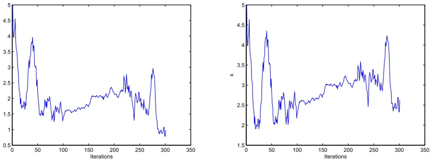
Because of the x-dependence in Q(x) given by (4.2), and the different stepsize used, the displays will not be the same. However, it can seen that with the same random seeds chosen, the sample paths display similar behavior. This suggests that the constant-stepsize approximation is a viable and easily implementable alternative as compared to the decreasing stepsize algorithms. In this example, we assume that the jump process has state space
M={1,2}, and the drift is a nonlinear function f(·,·) :R× {1,2} 7→R, where
f(x,1) = 2 + sinx, f(x,2) = 1 + sinxcosx.
The diffusion coefficients are given by
σ(x,1) = 0.5x, σ(x,2) = 0.2x.
We specify the initial conditions asx0 = 5 andα0 = 1, and use the constant stepsizeε= 0.01
and the decreasing stepsizes εn= 1/(n+99), respectively. The sample paths of the computed iterates are displayed in Figure 1.
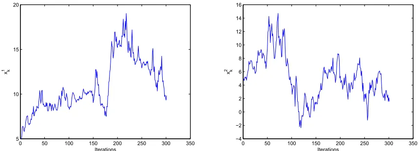
Example 4.3. In this example, we demonstrate the computational results of a process whose continuous component is two dimensional. For x = (x1, x2)′ ∈ R2, we use the x
-dependent generator Q(x) =Q(x1, x2) given by
Q(x1, x2) =
−5 cos
2x1−2 cos2x2 5 cos2x1+ 2 cos2x2
10 cos2x1+ 2 sin2x2 −10 cos2x1−2 sin2x2
.
Use the same constant stepsize as in the Example 4.2 for each dimension and specify the initial data as (x1
0 50 100 150 200 250 300 350 0.5
1 1.5 2 2.5 3 3.5 4 4.5 5
Iterations
x
(a) A sample path of approximation using constant stepsize algorithm
0 50 100 150 200 250 300 350 1.5
2 2.5 3 3.5 4 4.5 5
Iterations
x
[image:20.612.89.510.99.255.2](b) A sample path of approximation using a decreas-ing stepsize algorithm.
Figure 1: Sample paths for constant-stepsize and decreasing-stepsize algorithms
as follows:
σ(x1, x2,1) =
0.5x
1+ 0.2x2 0.003x1+ 0.001x2
0.007x1+ 0.008x2 0.47x1 + 0.3x2
,
σ(x1, x2,2) =
0.2x
1+ 0.3x2 0.001x1+ 0.002x2
0.008x1+ 0.005x2 1x1+ 0.5x2
,
f(x1, x2,1) =
2 + sinx
1+ cosx2
1 + cosx1+ cosx2
.
The sample paths are depicted in Figure 2.
For both of these examples, we have done a number of numerical experiments with different stepsize selections. They all produced similar sample path behavior as displayed above. For numerical experiment purpose, we have also tested different functions f(·,·) and
σ(·,·) as well. It is seen that our proposed algorithms are easily implementable and are suited for Monte Carlo studies.
5
Further Remarks
0 50 100 150 200 250 300 350 5
10 15 20
Iterations
x
1 k
(a) A sample path of the first component of the switching diffusion.
0 50 100 150 200 250 300 350 −4
−2 0 2 4 6 8 10 12 14 16
Iterations
x
2 k
[image:21.612.80.510.99.254.2](b) A sample path of the second component of the switching diffusion.
Figure 2: Sample paths of a 2-dimensional switching diffusion
constant stepsize algorithms, in which the state-dependent modulated switching process is approximated by a discrete-time switching process with state-dependent transition probabil-ities. Second, we proved the weak convergence of the proposed algorithm using a martingale problem formulation. We used continuity and localized analysis to overcome the difficulty of the state dependence. Third, we obtained existence and uniqueness of the switching dif-fusions. As a direct consequence, we obtain the strong convergence result in the sense of usual numerical solutions for SDE and established that the approximation sequence con-vergence strongly to the solution of the switching diffusion. Moreover, decreasing stepsize algorithms were developed as well. Finally, we provided examples to illustrate the utility of the approximation methods.
A number of problems deserve future study and investigation. Pursuing rates of conver-gence study is a worthwhile under-taking. Effort may also be devoted to numerical methods for regime-switching jump diffusions with state-dependent switching. Considering numerical methods for systems with delays and switching will be both interesting and important.
Acknowledgement. We thank the editors and reviewers for making many detailed com-ments and suggestions.
References
[1] G.K. Basak, A. Bisi, and M.K. Ghosh, Stability of a random diffusion with linear drift, J.
[2] K.L. Chung,Markov Chains with Stationary Transition Probabilities, 2nd Ed., Springer-Verlag, New York, NY, 1967.
[3] S.N. Ethier and T.G. Kurtz, Markov Processes: Characterization and Convergence, J. Wiley, New York, NY, 1986.
[4] D.J. Higham, X. Mao, and A.M. Stuart, Strong convergence of Euler-type methods for non-linear stochastic differential equations,SIAM J. Numerical Anal. 40 (2002), 1041-1063. [5] A.M. Il’in, R.Z. Khasminskii, and G. Yin, Singularly perturbed switching diffusions: rapid
switchings and fast diffusions,J. Optim. Theory Appl.,102 (1999), 555-591.
[6] N. Ikeda and S. Watable, Stochastic Differential Equations and Diffusion Processes, Springer, New York, 1981.
[7] Y. Ji and H.J. Chizeck, Controllability, stabilizability and continuous-time Markovian jump linear quadratic control,IEEE Trans. Automat. Control, 35(1990), 777-788.
[8] R.Z. Khasminskii, Stochastic Stability of Differential Equations, Sijthoff & Noordhoff, Alphen aan den Rijn, Netherlands, 1980.
[9] P.E. Kloeden and E. Platen,Numerical Solution of Stochastic Differential Equations, Springer-Verlag, 1992.
[10] H.J. Kushner, Approximation and Weak Convergence Methods for Random Processes, with applications to Stochastic Systems Theory, MIT Press, Cambridge, MA, 1984.
[11] H.J. Kushner and G. Yin, Stochastic Approximation and Recursive Algorithms and Applica-tions, 2nd Ed., Springer, New York, 2003.
[12] X. Mao, Stochastic Differential Equations and Applications, Horwood, 1997.
[13] X. Mao, Stability of stochastic differential equations with Markovian switching, Stochastic
Process. Appl.,79(1999), 45–67.
[14] X. Mao and C. Yuan, Stochastic Differential equations with Markovian Switching, Impreial College Press, London, 2006.
[15] M. Mariton, Jump Linear Systems in Automatic Control, Marcel Dekker, New York, 1990. [16] G.N. Milstein, Numerical Integration of Stochastic Differential Equations, Kluwer, New York,
1995.
[17] S.P. Sethi and Q. Zhang,Hierarchical Decision Making in Stochastic Manufacturing Systems, Birkh¨auser, Boston, 1994.
[18] A.V. Skorohod,Asymptotic Methods in the Theory of Stochastic Differential Equations, Amer-ican Mathematical Society, Providence, 1989.
[19] D.D. Sworder and J.E. Boyd,Estimation Problems in Hybrid Systems, Cambridge University Press, 1999.
[20] G. Yin and S. Dey, Weak convergence of hybrid filtering problems involving nearly completely decomposable hidden Markov chains,SIAM J. Control Optim.,41(2003), 1820-1842.
[21] G. Yin, R.H. Liu, and Q. Zhang, Recursive algorithms for stock Liquidation: A stochastic optimization approach,SIAM J. Optim.,13(2002), 240-263.
[22] G. Yin and Q. Zhang, Continuous-Time Markov Chains and Applications: A Singular Per-turbation Approach, Springer-Verlag, New York, 1998.
[23] C. Yuan and X. Mao, Asymptotic stability in distribution of stochastic differential equations with Markovian switching,Stochastic Process Appl.,103 (2003), 277–291.
[24] Q. Zhang, Stock trading: An optimal selling rule,SIAM J. Control. Optim.,40, (2001), 64-87. [25] C. Zhu and G. Yin, Asymptotic properties of hybrid diffusion systems, SIAM J. Control