Distributed Control of Multi-Robot Systems using Bifurcating Potential
Fields
Derek Bennet and Colin McInnes
Department of Mechanical Engineering
University of Strathclyde
Glasgow, G1 1XJ
{
derek.bennet, colin.mcinnes
}
@strath.ac.uk
Abstract— The distributed control of multi-robot systems has been shown to have advantages over conventional single robot systems. These include scalability, flexibility and robustness to failures. This paper considers pattern formation and recon-figurability in a multi-robot system using bifurcating potential fields. It is shown how various patterns can be achieved through a simple free parameter change. In addition the stability of the system of robots is proven to ensure that desired behaviours always occur.
I. INTRODUCTION
Over the past two decades distributed robot systems have been developed as a method of solving a variety of engineering problems [?]. Most of the research in this area is influenced by the early work of Brooks [?] in the mid
1980’s who introduced the concept of behavioural robotics. Although the majority of previous research had been concerned with single robot systems it was suggested that a significant step forward would be to draw on inspiration from nature and utilise the idea of emergent behaviour through decentralised control. This form of control has the advantages of being robust, scalable and flexible and has been applied to areas such a surveillance, exploration and transportation [?], [?].
The purpose of this paper is to investigate the distributed control of multi-robot pattern formation and reconfigurability. To achieve this we consider the use of the artificial potential field method and extend previous research by considering bifurcation theory in order to have a reconfigurable formation. Dynamical systems theory is used to demonstrate mathematically the stability of the system so that desired behaviours always occur.
Artificial potential fields were first introduced in Khatib [?] in the area of obstacle avoidance for manipulators and mobile robots. More recently they have been applied successfully in the area of autonomous robot motion planning [?], [?], as a form of distributed behavioural control in [?] and in space applications [?], [?], [?]. The basic idea behind potential field theory is to create a workspace where a robot is attracted towards a goal state with a repulsive potential ensuring collide avoidance [?]. As a multi-robot team may be required to achieve
different tasks a desirable property of the system would be reconfigurability. In order to minimise computational expense bifurcation theory can be used to reconfigure the formation through a simple free parameter change.
For real, safety critical applications it is essential that the behaviour of each robot is verified in order to ensure that no unwanted behaviours will occur. Winfield [?] has introduced the term ‘swarm engineering’ to highlight the key issues that are involved in real, safety critical applications as opposed to those based on simulation. Through the use of dynamical systems theory this paper aims to replace algorithm validation with mathematical proof in order to prove that desired formations always occur.
The paper proceeds as follows. In the next section we describe the model used and explain the artificial potential field method and bifurcation theory. We also discuss the linear and non-linear stability of the models developed. Section IIIshows the numerical results of simulations carried to demonstrate pattern formations and reconfigurability.
II. FORMATIONMODEL
We consider a system of homogeneous autonomous robots (1≤i≤N) interacting via an artificial potential functionU. It is assumed that all robots can communicate with each other and are fully actuated. The negative gradient of the artificial potential defines a virtual force acting on each robot so that the dynamics of each robot can be described by Eq. 1 and 2 with mass,m, position,xi, and velocity,vi;
dxi
dt =vi (1)
mdvi
dt =−∇iU
S(x
i)− ∇iUR(xij)−σvi (2)
From Eq. 2 it can be seen that the virtual force experienced by each robot is dependent upon the gradient of two different artificial potential functions and a dissipative term, where σ > 0 controls the amplitude of the dissipation. The first term in Eq. 2 is defined as thesteering potential,US which
The repulsive potential is based on a generalized Morse potential [?] as shown in Eq. 3;
UijR=
X
j,j6=i
Crexp−|xij|/Lr (3)
Where Cr and Lr represent the amplitude and
length-scale of repulsive potential respectively and|xij|=|xi−xj|.
The total repulsive force on the ith robot is dependent
upon the position of all the other (N −1) robots in the formation. The repulsive potential is therefore used to ensure that as the robots are steered towards the goal state they do not collide with each other. Once all the robots have been driven to the desired equilibrium state the repulsive potential also ensures that they are equally spaced for symmetric formations.
A. Artificial Potential Function Scale Separation
As noted in the previous section the force experienced by each robot is dependent upon the gradient of two different ar-tificial potential functions. The steering potential is a function of position only. We now consider a supercritical pitchfork bifurcationequation in Eq. 4, with bifurcation parameter µ and length scale R. A detailed explanation of this steering potential is given in section II B. The repulsive potential noted in the previous section is given in Eq. 5;
US = −12µ(X−R)2+1
4(X−R)
4
(4)
UR=Crexp−X/Lr (5)
For illustration we consider a simple 1-dimensional system with position coordinateX.
Defining an outer region dependent upon the steering potential only and an inner region dependent upon the repulsive potential only we can show that these two regions are separated so that the robot move under the influence of the long-range steering potential, but with short range collisions (for Lr/R <<1) effectively creating a boundary
layer between them. This can then be used to determine the non-linear stability of the system considering the steering potential only.
For 1D motion of a robot of massmwe have;
mdV
dt = − ∂UR
∂X − ∂US
∂X −σV (6) So that,
mV dV dX =
Cr
Lrexp −X/Lr
+µ(X−R)−(X−R)3−σV (7)
ScalingX such thatS=X/Rthen;
1
RmV dV dS =
Cr
Lr
exp−
R Lr
S
+µR(S−1)−R3(S−1)3−σV (8)
Now defineε= Lr
R <<1 so that;
mVdV dS =
Cr
ε exp
−S
ε
+R
µR(S−1)−R3(S−1)3−σV
(9)
Letε→0 in order to consider ‘far field’ dynamics which forms a singularly perturbed system;
lim
ε→0
1
εexp
(−S/ε)= 0
(10)
Therefore at large separation distances the repulsive potential vanishes and we can consider the steering potential only when considering the stability of analysis of the system.
Conversely if we define S = S
ε we find that the ‘near field’ dynamics are defined by;
mVdV
dS = Crexp
−S+
εR
µR(S−1)−R3(S−1)3−σV
(11)
and lettingε→0;
mVdV
dS =Crexp
−S
(12)
Thus, at small separations the steering potential vanishes and we can treat the collisions separate in the subsequent stability analysis.
B. 1-Parameter Static Bifurcation
Referring back to Eq. 2 thesteering potentialcan be based on asupercritical pitchfork bifurcation[?] as shown in Eq. 13. The aim of this potential is to drive each robot to a goal distance,r, from the origin in the x-y plane thus forming a symmetric ring.
US(xi;µ, α) = −
1
2µ(ρi−r)
2
+1
4(ρi−r)
4
(13)
Whereρi = (x2i +yi2)0.5.
0 0.5 1 1.5 2 2.5 3 3.5 4 4.5 5
-6 -4 -2 0 2 4 6 8
ρeq
µ
Stable
Unstable Stable
[image:3.612.41.273.9.233.2]Stable
Fig. 1. Supercritical pitchfork bifurcation diagram
0 10 20 30 40 50 60
0 1 2 3 4 5 6 7 8
ρ
U
-6 -4 -2 0 2 4 6 8 10 12 14
0 1 2 3 4 5 6 7 8
ρ
U
[image:3.612.307.542.263.411.2](i) (ii)
Fig. 2. Potential functions: (i)µ <0and (ii)µ >0
The equilibrium states of the potential occurs whenever ∂U/∂ρi= 0. Therefore;
∂U ∂ρi
=−µ(ρi−r) + (ρi−r)3 (14)
If µ ≤ 0 equilibrium occurs when ρi = r. If µ > 0
equilibrium occurs when ρi = r, r ±√µ. Therefore, a
single ring will bifurcate to a double ring using µ as a control parameter.
The stability of the potential is determined from the sign of the second derivative, given in Eq. 15, and summarised in Table I;
∂2U
∂ρ2
i
=−µ+ 3(ρi−r)2 (15)
TABLE I
STABILITY OF EQUILIBRIUM STATES
Bifurcation Equilibrium ∂2U/∂ρ2
i Stability
parameter,µ position,ρeq
<0 r >0 stable minimum
>0 r <0 unstable maximum
r+√µ >0 stable minimum r−√µ >0 stable minimum
1) Linear stability:1-parameter static bifurcation: In or-der to determine the linear stability of a system of robot sub-ject to such a 1-parameter bifurcation steering potential we perform an eigenvalue analysis on the linearized equations of motion assuming that at large separation distances the repulsive potential can be neglected through scale separation as explained insection II A. The linear stability analysis will be used to determine the local behaviour of the system by
calculating its eigenvalue spectrum. Therefore, the equations of motion for the model are re-cast as;
˙
xi
˙
vi
=
vi
−σvi− ∇iUS(xi)
=
f(xi,vi)
g(xi,vi)
(16)
Let xo and vo denote fixed points with x˙i = ˙vi = 0 so
that;
f(xo,vo) = 0 (17)
g(xo,vo) = 0 (18)
Thus,vo = 0 and∇US = 0 at equilibrium. This occurs
when ρo = r if µ < 0 and ρo = r, r±√µ if µ > 0.
Defining δxi = xi −xo and δvi = vi −vo and Taylor
Series expanding about the fixed points to linear order the eigenvalues of system can be found using;
δx˙i
δv˙i
=J
δxi
δvi
(19)
where,
J=
∂
∂xi(f(xi,vi)) ∂
∂vi(f(xi,vi)) ∂
∂xi(g(xi,vi)) ∂
∂vi(g(xi,vi))
xo,vo
(20)
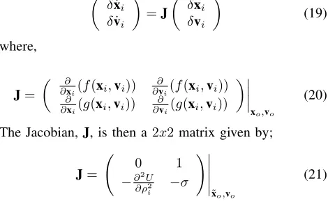
The Jacobian,J, is then a2x2matrix given by;
J= 0 1
−∂∂ρ2U2 i −σ
! ˜x
o,vo
(21)
Substituting a trial exponential solution into Eq. 19 we find that;
δxi
δvi
=
δxo
δvo
eλt (22)
Therefore, the eigenvalues, λ, of the system are found
fromdet(J−λI) = 0.
As shown previously, ifµ <0 equilibrium of the system occurs whenxo= (r,0)andvi= 0. Evaluating the Jacobian
matrix given in Eq. 21 we find that;
J=
0 1
µ −σ
(23)
The corresponding eigenvalue spectrum is therefore;
λ= 1/2(−σ±p
(σ2+ 4µ)) (24)
As σ > 0 and µ < 0 the eigenvalues are always either negative real or complex with negative real part as −σ±p
(σ2+ 4µ) ≯ 0. The equilibrium position can
If µ > 0 equilibrium of the system occurs when xo1 =
(r,0),xo2= (r+√µ,0)andxo3= (r−√µ,0)withvi= 0.
The Jacobian matrix evaluated at the three different equilib-rium positions is given by Eq. 25, 26 and 27 respectively as;
J1=
0 1
µ −σ
(25)
J2=
0 1
−2µ −σ
(26)
J3=
0 1
−2µ −σ
(27)
The eigenvalues forJ1 are;
λ= 1/2−σ±p
(σ2+ 4µ) (28)
Considering the pair of eigenvalues in Eq. 28 we can show that −σ±p
(σ2+ 4µ) > 0 since, σ2+ 4µ > σ2
and therefore we always have atleast one positive real eigenvalue. This equilibrium position is therefore always linearly unstable.
The eigenvalues forJ2 andJ3are;
λ= 1/2−σ±p(σ2−8µ) (29)
Again as σ > 0 and µ > 0 the eigenvalues are always either negative real or complex with negative real part as −σ± p(σ2−8µ) ≯ 0. The equilibrium positions can
therefore be considered as linearly stable.
2) Non-linear stability: 1-parameter static bifurcation: To determine the non-linear stability of the dynamical system we consider Lyapunov’s Second Theorem as expressed by Kalman and Bertram[?], [?] ;
“If the rate of change ofdE(x)/dtof the energyE(x)of an isolated physical system is negative for every possible state x, except for a single equilibrium state xe, then the energy will continually decrease until it finally assumes its minimum valueE(xe)”
The aim of the steering potential is to drive the robot to the desired equilibrium position that corresponds to the minimum potential. Therefore, if Lyapunov’s method can be used for the system, as time evolves the system will relax into the minimum energy state.
The Lyapunov function,L, is defined as the total energy of the system, where US(x
i)is given in Eq. 13 so that for
unit mass;
L=X
i
1
2v
2
i +US(xi)
(30)
Where,L >0other than at the goal state whenL= 0.
The rate of change of the Lyapunov function can be expressed as;
dL dt =
∂L
∂xi
˙
xi+
∂L
∂vi
˙
vi (31)
Then, substituting Eq. 16 into Eq. 31 it can be seen that;
dL dt =−σ
X
i
v2i ≤0 (32)
From Lyapunov’s Second Theorem [?] it states that if L is a positive definite function and L˙ is a negative definite the system will be uniformly stable. A problem arises in the use of superimposed artificial potential functions asL˙ ≤0. This implies that L˙ could equal zero in a position other than the goal minimum suggesting that the system may become trapped in a local minimum. In order to ensure that our system is asymptotically stable at the desired goal state the LaSalle principle [?] can be used. It extends the above constraints to state that if L(0) = ˙L(0) = 0 and the set {xi|L˙ = 0}only occurs whenxi=xo, then the goal state is
asymptotically stable. Therefore, for the quadratic potential considered in this paper the LaSalle principle is valid. As we have a smooth well defined symmetric potential field, equilibrium only occurs at the goal states so the local minima problem can be avoided and the system will relax into the desired goal position.
C. 2-parameter Static Bifurcation
An extension to the 1-parameter pitchfork bifurcation is to consider 2-parameter bifurcations such as the so-called cusp catastrophe given in Eq. 33. Fig. 3 shows the variation of the equilibrium position with the two parameters,µ1 andµ2.
U(ρi;µ1, µ2) =µ1(ρi−r)2+ (ρi−r)4+µ2(ρi−r) (33)
0 5 10
Ρ
-10 0 10
Μ1
-20 0
20
[image:4.612.47.285.80.206.2]Μ2
Fig. 3. Cusp catastrophe surface [?]
Mapping the cusp potential onto the µ1−µ2 plane we
2 1
0 0
2
1
[image:5.612.101.217.8.137.2]1
1
Fig. 4. Mapping of equilibrium on µ1-µ2 plane showing number of equilibrium states (rings)
If we setµ2= 0 we have the usual pitchfork bifurcation
equation. However, forµ1>0and allµ2 we only have one
equilibrium position. For µ1 < 0 and for all µ2 we have
either 1 or 2 equilibrium states as shown. If we hold µ1
at a constant negative value and alternateµ2 from negative
to positive we obtain a hysteresis loop alternating between one and two equilibrium positions. We can therefore tip the system into the upper or lower branches of the pitchfork equation as shown in Fig. 5. Thus if the system is in the bi-stable state, control over the position of a single minimum state can be achieved through the variation of the parameters in the bifurcation equation.
-6 -4 -2 0 2 4 6 8 10 12 14
0 1 2 3 4 5 6 7 8
ρ
U
(i)
0 10 20 30 40 50 60 70 80 90 100
0 1 2 3 4 5 6 7 8 9
ρ
U
-30 -20 -10 0 10 20 30
0 2 4 6 8 10
ρ
U
(ii) (iii)
Fig. 5. Cusp catastrophe: (i)µ1 <0,µ2 = 0(ii)µ1 <0,µ2>0(iii) µ1<0,µ2<0
D. Rotation of the Formation
Recent work by McInnes [?] has shown how vortex like swarming can be achieved through artificial potential field methods. Eq. 1 and 2 are now modified to include a dissipative orientation term as shown in Eq. 34 and 35. Eq. 36 shows the orientation term that dissipates energy whilst aligning the velocity vectors of members of the swarm where Co and Lo are constants representing the magnitude and
length-scale of the dissipation;
dxi
dt =vi (34)
mdvi
dt =−Λi− ∇iU
S(x
i)− ∇iUR(xij) (35)
Λi=
X
i6=j
Co(vij.ˆxijexp−|xij|/lo)ˆxij (36)
The emergence of vortex like formations can be seen through the conservation of angular momentum,H;
X
i
xi×mv˙i =
d dt
X
i
(xi×mvi)
= dH
dt = 0 (37) It can also be shown that as time evolves the system of robots will relax into the minimum energy,E, state where
P
ivi · Λi = 0. The swarm therefore dissipates energy
while conserving angular momentum and so relaxes into the rotating ring[?] wherevij·ˆxij= 0.
III. NUMERICALRESULTS
[image:5.612.342.538.106.157.2]A. Static Bifurcation Formation Patterns
Fig. 6 shows the three different robot formations that can be formed using a 1 parameter static bifurcation. The system considers a swarm of30 robots with unit mass and σ= 10.
−2 −1 0 1 2
−2 −1.5 −1 −0.5 0 0.5 1 1.5 2
x
y
(i)
−5 −4 −3 −2 −1 0 1 2 3 4 5 −5
−4 −3 −2 −1 0 1 2 3 4 5
x
y
−6 −4 −2 0 2 4 6 −6
−4 −2 0 2 4 6
x
y
[image:5.612.39.280.334.507.2](ii) (iii)
Fig. 6. Formation patterns: (i) cluster (Cr= 1,Lr= 0.5andµ=−4 (ii) ring (Cr= 1,Lr= 0.2,r= 3andµ=−4) (iii) two rings (Cr= 1, Lr= 0.5,r= 3andµ= 1.5)
The first formation corresponds to the case whenµ=−4
and r = 0. The robots are driven towards the origin with the repulsive potentialultimately causing a uniform cluster to form. The second formation consists of a ring with the radius of the ring determined by the magnitude that the steering potentialhas been moved along theρi-axis (in this
[image:5.612.308.527.338.541.2]µ= 1.5. The stable equilibrium state in the second formation has become unstable and the system bifurcates into two rings.
B. 1-Parameter Static Bifurcation
Figures 7 shows the transition of a formation of30robots in the x-y plane. As it can be seen, the system changes from a ring to two rings to a cluster then back to a ring. This is achieved through a simple parameter change and is one of the advantages of using the pitchfork bifurcation equation as a basis for the artificial potential function. Rather than controlling each robot individually the global pattern of the formation can be manipulated viaµ.
-4 -2 0 2
4 -5
0 5 0 50 100 150
x y
ti
m
e
Two Rings:
µ = 2, r = 2
Ring:
µ = -2, r = 2
Cluster:
µ = -2, r = 0
Ring:
[image:6.612.337.501.102.274.2]µ = -2, r = 2
Fig. 7. Transition between different formations withσ= 1
C. 2-Parameter Dynamic Bifurcation
Figure 8 demonstrates how a 2-parameter bifurcation can be used to manipulate a robot formation. As can be seen if we start in the two ring case when µ1 = −2 and µ2 = 0
and then varyµ2, therefore performing a bifurcation on the
system, we can either tip the system into a large or small ring.
-4 -2 0
2 4
-5 0 5 0 10 20 30 40 50 60 70 80
x y
ti
m
e
Two Rings:
µ1 = -2, µ2 = 0
Inner Ring:
µ1 = -2, µ2 = 2
Outer Ring:
[image:6.612.78.244.179.346.2]µ1 = -2, µ2 = -2
Fig. 8. Evolution of cusp catastrophe results
D. Rotation of the Static Bifurcation Formation
Figures 9 shows the rotation of the ring formation using Eq. 36. The formation relaxes into to a single ring and conserves angular momentum by rotating about its centre of mass.
-10 -5 0
5 10
-10 0 100 50 100 150
x y
ti
m
e
Fig. 9. Time evolution of vortex ring
IV. CONCLUSION
We have shown that the control of a multi-robot system can be achieved through the use of the artificial potential function method. We have extended previous research in this area through the use of bifurcation theory to demonstrate that through a simple parameter change a formation of robots can be made to alter their configuration and shown how 1 and 2 parameter static bifurcations can be used to this effect. An important step in real engineered systems is to ensure that the formation can form reliably. Through dynamical systems theory we have demonstrated the stability of a system of robots driven to the equilibrium position to ensure that desired behaviours always occur. Future work will consider generalising the potential function method in order to achieve arbitrary patterns whilst also considering nonholonomic constraints in order to make the model more realistic.
REFERENCES
[1] Parker L.E. Current state of the art in distributed autonomous mobile robotics.in Distributed Autonomous Robotic Systems, L. E. Parker, G. Bekey, and J. Barhen eds., Springer-Verlag Tokyo, Vol. 4:3–12, 2000. [2] Brooks R. A. A robust layered control system for a mobile robot.IEEE
Journal Of Robotics And Automation, Vol. 2, No. 1:14–23, 1986. [3] Bahceci E., Soysal O., and Sahin E. A review: Pattern formation
and adaptation in multirobot systems. InRobotics Institute, Carnegie Mellon University, , Tech. Rep. CMU-RI-TR-03-43, Pittsburgh, PA, October 2003.
[4] Song P. and Kumar V.R. A potential field based approach to multi-robot manipulation. InIEEE International Conference on Robotics and Automation Volume 2 pages 1217-1222, 2002.
[image:6.612.75.247.490.655.2][6] Badaway A and McInnes C.R. Robot motion planning using hyper-boloid potential functions. In In: World Congress on Engineering, London, UK, July 2-4, 2007.
[7] Ge S.S. and Cui Y.J. Dynamic motion planning for mobile robots using potential field method. Autonomous Robots, Vol. 13:207–222, 2002.
[8] Reif J.H. and Wang H. Social potential fields: A distributed behavioral control for autonomous robots.Robots and Autonomous Systems, Vol. 27, No. 3:171–194, 1999.
[9] Bennet D.J. and McInnes C.R. Pattern transition in spacecraft formation flying via the artificial potential field method and bifurcation theory. In3rd International Symposium on Formation Flying, Missions and Technologies, Noordwijk, The Netherlands, April 23-25, 2008. [10] A. Badawy and C.R. McInnes. On-orbit assembly using superquadric
potential fields.Journal of Guidance, Control, and Dynamics, Vol. 31, No. 1:30–43, 2008.
[11] Izzo D. and Pettazi L. Autonomous and distributed motion planning for satellite swarm.Journal of Guidance, Control, and Dynamics, Vol. 30, No. 2:449–459, 2007.
[12] Winfield A, Harper C, and Nembrini J. Towards dependable swarms and a new discipline of swarm engineering. InSAB Swarm Robotics Workshop, Santa Monica, July 17, 2004.
[13] D’Orsogna M. R, Chuang Y. L, Bertozzi A. L, and Chayes S. The road to catastrophe: stability and collapse in2d driven particle systems.
Physical Review Letters, Vol. 96, No. 10:14302–1, 2006.
[14] Jordon D.W. and Smith P.Nonlinear Ordinary Differential Equations: An Introduction to Dynamical Systems. Oxford University Press, p432, 1999.
[15] Kalman R. E. and Bertram R. E. Control system analysis and design via the second method of lyapunov part i: Continuous systems.Trans. ASME, Vol. 82:371–393, 1960.
[16] Kalman R. E. and Bertram R. E. Control system analysis and design via the second method of lyapunov part ii: Discrete systems. Trans. ASME, Vol. 82:394–400, 1960.
[17] LaSalle J. P. The invariance principle in the theory of stability.Centre for Dynamical Systems, Brown University (NASA Technical Report), June 23, 1966.
[18] Weisstein E. W. Wolfram web resource: Cusp catastrophe.
www.mathworld.wolfram.com, 27/10/2007.
[19] Cengel Y.A and Turner R.H.Fundamentals of Thermo-Fluid Sciences. McGraw-Hill, 2001.
[20] McInnes C. R. Vortex formation in swarms of interacting particles.
![Fig. 3.Cusp catastrophe surface [?]](https://thumb-us.123doks.com/thumbv2/123dok_us/1690289.122393/4.612.47.285.80.206/fig-cusp-catastrophe-surface.webp)


