City, University of London Institutional Repository
Citation: Pizza, M. and Strigini, L. (1998). Comparing the effectiveness of testing
methods in improving programs: the effect of variations in program quality. Paper presented at the The Ninth International Symposium on Software Reliability Engineering, 4 - 7 Nov 1998, Paderborn, Germany.
This is the unspecified version of the paper.
This version of the publication may differ from the final published
version.
Permanent repository link: http://openaccess.city.ac.uk/265/
Link to published version:
Copyright and reuse: City Research Online aims to make research
outputs of City, University of London available to a wider audience.
Copyright and Moral Rights remain with the author(s) and/or copyright
holders. URLs from City Research Online may be freely distributed and
linked to.
City Research Online: http://openaccess.city.ac.uk/ [email protected]
9th International Symp. on Software Reliability Engineering, ISSRE '98, Paderborn, Germany © 1998 IEEE. Personal use of this material is permitted. However, permission to reprint/republish this material for advertising or promotional purposes or for creating new collective works for resale or redistribution to servers or lists, or to reuse any copyrighted component of this work in other works must be obtained from the IEEE.
Comparing the Effectiveness of Testing Methods in Improving
Programs: the Effect of Variations in Program Quality
Michele Pizza
Lorenzo Strigini
Centre For Software Reliability
City University, London, England
Abstract
We compare the efficacy of different testing methods for improving the reliability of software. Specifically, we use modelling to compare "operational" testing, in which test cases are chosen according to their probability of occurring in actual use of the software, against "debug" testing methods, in which the testers look for test cases which they consider likely to cause failure, or that satisfy some coverage criterion.
We base our comparisons on the reliability reached by the program at the end of testing. Differently from previous studies, we consider the probability distribution of the achieved reliability, and thus the probability of satisfying specific requirements, rather than just the average reliability achieved. We take account of two sources of variation: the variation between the actual test histories that are possible for a given program and a given test method; and the fact that different programs start testing with different faults and initial reliability levels. By necessity, we use very simplified models of reality. Yet, we can show some interesting conclusions with important practical consequences. In general, there are stronger arguments in favor of operational testing than previous studies have shown.
1. Introduction
We are interested in testing as a means for improving the reliability of delivered software. Testing is commonly considered essential for achieving adequate reliability, by removing bugs before delivering a product, but is an expensive activity.
There is demand for systematic testing methods (i.e., criteria for choosing test cases and possibly stopping rules), giving some guarantee of thoroughness and cost-effectiveness. Popular methods include those that systematically select test cases that are considered likely to produce failure (e.g., boundary case testing), and those that aim at a high "coverage", e.g. of parts of the code or of the specification. We will call these methods, collectively, "debug" testing methods, and compare them with what we call "operational" testing: choosing test cases to be statistically representative of intended use of the software.
Advocates of operational testing can point to these main advantages:
• it tends to discover defects which would cause frequent failures before those that would cause less frequent failures. So, it focuses correction efforts in the most cost-effective way and may deliver better software for a given debugging effort;
• it facilitates the automation of the test process, thus allowing more testing at acceptable cost than manual testing would allow;
• it directly supports estimates of reliability, and thus decisions on whether the software is ready for delivery or for use in a specific system. This feature is unique to statistical testing.
Advocates of "debug" testing methods can point out that an experienced human tester must be better than mere chance at finding bugs. A tester using a debug testing method (called the "debugger" in the rest of this paper) will tend to choose test cases that are very likely to cause failures, if bugs are present in the program.
Clearly, which method is actually better in a specific case must depend on whether the debuggers' intuition, if indeed better in finding bugs than mere random choice of test cases, guides them to discover those bugs that contribute heavily to unreliability, so that the correction effort is cost-effective.
Several authors have published comparisons between classes of testing methods [1-9]. Experimental comparisons have been inconclusive so far. Among comparisons based on modelling, we think the most advanced so far is in [8, 9], to which we refer the reader for more extensive background material and whose analysis we seek to extend.
testing methods that appear promising because of their ability to detect many faults may well be vastly inferior to operational testing, unless they preferentially discover the more important faults.
Most of the results published so far concerned comparisons of the expected values of the reliability achieved by testing. In this paper, we study the
distribution of the achieved reliability, i.e., the
probabilities of achieving specified reliability levels.
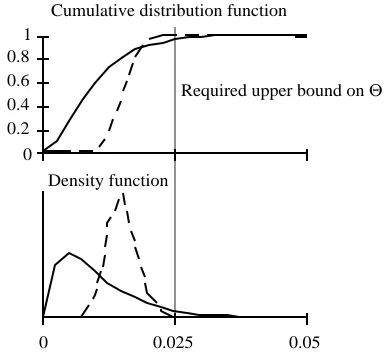
Method A (solid line): E(Θ)=0.01; P(Θ>0.025)=0.04 Method B (dashed line): E(Θ)=0.015; P(Θ>0.025)=0.00082
Density function
0 0.025 0.05
Cumulative distribution function
0 0.2 0.4 0.6 0.8 1
[image:3.595.72.264.180.358.2]Required upper bound on Θ
Fig. 1: Trade-off between average results and consistency of results in two hypothetical statistical distributions of t h e failure rates (Θ) obtained after testing.
Comparing expected values is potentially misleading. In reality, the history of testing in a specific project will differ from all others. The reliability achieved on average may well matter less than the predictability of the results. For instance, of the two hypothetical methods shown in Fig. 1, method A delivers better average reliability, but method B is more dependable, as it has a smaller "tail" of programs that are worse than a required bound.
There are actually two main sources of variation among the results obtained by applying a given method:
- first, in the application of a given method to a given
program, we can consider the factors that might differ
between two applications of the method, e.g.: different choices of tests by different testers, different random effects in the testing environment (e.g. load), and the fact that the tester[s] may react differently to observing a failure, in terms of how they will proceed to look for the fault and attempt to repair it. Most previous investigations have considered this scenario;
- another source of uncertainty, though, is that a testing method chooses test cases on the basis of some characteristics of a program, but cannot be specialized to the individual program actually being tested. For instance, if one tests for coverage of features in a specification document, the same choice of tests applies to all programs that nominally satisfy the same
specification; a debugger, having to choose a test within the constraints specified by a testing method, will choose a test for its presumed efficacy at detecting possible faults in that specific program, based on
general experience with similar programs. But
programs which share these general outwards characteristics will normally differ in the faults they contain, and the testing method will thus achieve different levels of reliability in different programs. We might thus have that testing method A tends to be much better than method B if the program happens to contain certain bugs, but worse than B if the program has bugs of a different kind. The program characteristics that drive the choice of test cases identify a whole
population of programs that might have been produced,
with individual differences including different faults. The program actually tested is one of these programs, but the testers do not know which one. Decisions about testing must make allowance for this uncertainty. Statistically, these differences among the testing histories that are possible with a given test method are described as a probability distribution for the reliability achieved at the end of testing. Many scenarios are possible, with bafflingly subtle variations. Just to give an example, we may consider that the reliability of programs before testing has a given statistical distribution. Suppose that the dominant categories of bugs in programs were correlated with the program's reliability. We might then find that a testing method is very good (statistically) at improving bad programs, but ineffective on programs that are already reasonably reliable; or that another testing method usually improves those programs that are already rather good, but rarely improves the worse programs. The latter method would deliver programs that after testing vary more widely in reliability than they did before testing; the former method would instead reduce this spread, thus making the software development process more predictable and controllable.
Our second source of variation was not usually modelled in previous studies of testing methods. Yet, it is important for at least two practical reasons:
- if we model the testing process to gain general insight, so that we may understand which factors determine which method is more successful, we will normally model the ability of a tester as a probability of finding faults in a program. But if we consider the variation among programs, we will recognize that a good tester is one who achieves a good average score over all programs that appear similar. The tester's ability cannot be calibrated on the faults of the specific program now under test, which are as yet unknown. The difference between effectiveness on the average program and on the individual programs will be demonstrated by an example in Section 5;
3
test process on a small sample of programs, we will be tempted to judge those test inputs that do not reveal defects as "wasting" tests and thus lowering the value of the testing method or of the tester. But our considerations have shown that this would be wrong. A test case which does not reveal any defect in a specific program A may well be a test case which would reveal a fault frequently present in other programs similar to A. Any inference obtained from a small sample of programs needs to allow for the natural variation among programs. The programs in the sample may be very different from the "typical" program in the population of similar programs. A "typical" program may well not exist at all.
This description of the variation in the testing process may give an impression of hopeless complexity, such that no general law and no directive for empirical investigation can be found. We describe here preliminary attempts at exploring the problem and deriving useful conjectures, via a few thought experiment. First, we propose models of how software faults are distributed in programs, and how tests find them, that account for specific, interesting aspects of reality. So, we can study the consequences of these aspects. For some models, we have been unable so far to produce analytical solutions, so we describe single examples, solved numerically. We can thus discuss general conjectures about the behavior of testing methods in practice. Of course, our models ignore many aspects of reality. It is important to decide whether our conclusions are indeed due to those model assumptions that are realistic, or are an artefact without a basis in reality. Even with these limitations, we think these models contribute to a better understanding of the phenomena to be studied. We hope that practitioners can use our conclusions in deciding how to proceed in their particular situations, and researchers to guide experimental efforts.
2. Terminology and assumptions
2.1. Testing, faults, failures
In the scenario we consider, a program is tested by giving it a stimulus, and checking whether its reaction is correct. We call the stimulus test input, test case or just
test and the response output. This intuitively describes a
state-less program which implements a function (in the mathematical sense of the word), but can also represent more complex situations. For instance, for a control system with a defined mission time, a whole mission can be one test case; for a transaction-processing system, the state of its data base must be considered as part of each input; etc. The set of all variables that affect one invocation of the program defines a multidimensional, discrete, Cartesian input space.
If the program reacts correctly to a test, we call this event a success; if not, we call it a failure. Failures are due to the presence of faults in the program. In discussions of testing, faults (or "defects", or "bugs") are usually thought of as those parts of the code that are wrong. This
definition does not allow a unique identification of the faults in a program (in general, there are many different code changes which would all correct the same set of incorrect behaviors), so we prefer to characterize a program's faults via its failure set, defined as follows. A
failure point is a point in the input space of the program,
such that the program behaves incorrectly on that input. A
failure region is any set of failure point that we think
convenient to consider together, e.g., all the failure points that would be eliminated by a given fix. The failure set of the program is the set of all its failure points, i.e., the union of all its failure regions.
We describe the [un]reliability of a program in terms of its failure rate (or failure probability), i.e., in this context, the probability that the program fails on an input if this is chosen at random from the input space, according to the probability distribution that would be observed in actual operation.
2.2. Simplified model of program development
We need to model the evolution of a program during its history of testing and repair. We start with describing how faults are inserted, and how failure behaviors vary over a population of similar programs.
We know from experience that a mistake by a developer will not usually affect a single input point, but a whole set. If the mistake is made, the whole set of points becomes a failure region; if not, the failure region will not be there. So, a simple model assumes a fixed (potentially huge) set of possible failure regions, corresponding to the mistakes that developers may make. The accidental errors in the design process select some of these failure regions, at random. We characterize each "potential failure region" by its probability (shorthand for the probability of that failure region actually being in the program), and its size or failure rate (shorthand for the decrease in the program's failure rate achieved by a fix that turns all and only the points in that failure regions into success points). So, for instance, we may talk about a "large, improbable" failure region to mean a failure region that is unlikely to be present, but if present causes frequent failures in operation. In our examples, we will make a series of assumptions to keep our models tractable, especially when numerical solutions are needed:
- there is a finite number N of classes of possible failure regions: class i has ni elements, each of size qi and with probability pi. This is not overly restrictive, but in practice we will use small values for N and each ni to keep our examples tractable. Such assumptions seem acceptable approximations for scenarios like those found in simple, safety critical software, with good development quality, in which one may expect most programs to have very few defects: although many other failure regions might be present in theory, only a few have a high enough probability to affect the statistics of the developed programs;
failure regions. This is not true in practice, but again, it should be a realistic approximation for cases in which few, small failure regions are usually present. We also assume that the presence of a failure region (or, equivalently, the mistake that causes it to be present) is statistically independent of the presence of any other. This is as though the design team tossed dice, for each failure region to decide whether to insert it or not.
2.3. Model of the testing and fixing process
During testing, any detected failure is followed by an attempt to identify its cause and remove it by fixing the software. We use the following simplifying assumptions, common to most existing models of testing:
- each successive test selection is independent of all the ones preceding it and chosen according to the same probability distribution;
- failures (resp. successes) are always recognized as failures (resp. successes). In the jargon of testing research this is called the perfect oracle assumption; - when a failure happens, the testers deterministically
change the code so as to remove that failure region, among the collection we specified before, to which the test input that caused the failure belongs. So, we ignore the fact that in reality different testers may apply different fixes, even when responding to identical test failures (perfect and identical fixes).
Our models are heavily stylized descriptions of reality (see e.g. [9, 8] for a discussion of why they may not be verified in practice). Yet, we are not using them for detailed predictions, but for pointing at the existence of phenomena that are usually ignored. So, they will suffice as long as the phenomena we demonstrate are not a consequence of those specific assumptions that are unrealistic.
di detection rate in debug testing for each failure
region of class i
d value of di when it is assumed to be the same for
all failure regions
E(X) expected value (mean) of a random variable X
ni number of possible failure regions in the i-th
class (i=1,...,N)
N number of classes of possible failure regions
pi probability that one failure region of class i is
actually present in a randomly chosen program
P(Α) probability of an event A
qi failure rate in actual operation for each failure
region of class i
t number of tests performed
Θ "Failure rate" of a program: probability of it
failing on an input chosen at random according to the probability with which it will occur in operation in the environment of interest
Θo(t) or
Θo, Θd(t) or Θd
'failure rate' of a program after t tests have been run and all defects found have been corrected, with operational and debug testing respectively
Abbreviations used in this article
3. Testing without subdomains
Here, we consider the case in which the debugger does not divide the input space into subdomains but uses some kind of heuristic to seek those input points that are more likely to be failure points. We focus on a case in which the debugger’s detection rate is the same for each of the program’s failure regions: di=d for every i. We do not believe this to be a "typical" situation: we think there is no empirical basis for believing that a "typical" situation exists, common to all practical industrial contexts. However, this scenario produces examples which are worth studying. In reality, we would expect di to be highly variable, and it might be either positively or negatively correlated with the failure rates of the failure regions, depending on the testers and the program types. Assuming it constant (as other authors have done before us) is the simplest case for a first mathematical analysis.
3.1. One class of failure regions
Let us assume that there is only one class of potential failure regions. All regions have the same probability of being actually present and the same failure rate in operation: N=1, q1=q, p1=p, n1=n, and Θ can thus only take values in the set: {0, q, 2 q,...nq}.
3 . 1 . 1 . D e r i v i n g t h e probability distribution of the failure rate Θ after testing
We briefly show how to obtain the distribution of the failure probability Θ after t tests. Since Θ equals the number r of failure regions left in the program times their individual failure rate, q, it is sufficient to compute the probability of each possible value of r. So, for debug testing, after t tests:
P(Θd=r q) = P(r failure regions in the program)=
k=r n
∑ P(r failure regions | k failure regions before testing) P(k failure regions before testing) The rightmost term represents a binomial distribution: P(k failure regions before testing)= n
k ⋅ k
p⋅
(
1−p)
n−k, and the other term in each product is:P(r failure regions | k failure regions before testing)=
∑
α=0 t
P(r failure regions | α test hits, k failure regions before testing) P(α test hits | k failure regions before testing)
(where a "test hit" is defined as a test hitting a point in one of the failure regions initially present). In their turn, the two terms in this sum can be written as:
P(α test hits | k failure regions before testing)= t
α
5
(another binomial distribution) and ([11], vol. 3, p. 60): P(r failure regions | α test hits, k failure regions before
testing)= k r
⋅ x (−1) ⋅ x=0 k−r
∑ kx−r ⋅ 1−r+x k
α
For operational testing, the only change is that the probability of finding a failure region is q instead of d:
P(Θo=r q)=
x (−1)⋅ x=0 k−r
∑ kx−r ⋅ 1−r+x k
α α=0 t ∑ k=r
n ∑ ⋅ t α
( )
k⋅qα⋅(
1−k⋅q)
t−α⋅ nk
⋅pk⋅
(
1−p)
n−kThe means of these two distributions are easily derived:
Θ is the sum of n random variables, each representing the contribution of one of the potential failure regions. With debug testing, after t tests the program contains on average
np(1-d)t failure regions, thus the expected failure rate is:
E(Θd)=q⋅n⋅p⋅(1−d)t
With operational testing, this becomes: E(Θo)=q⋅n⋅p⋅(1−q)t
With many classes of failure regions, the expressions of these probability distributions become more complex. In practice, we evaluated the probabilities of all possible sets of remaining failure regions incrementally through successive steps in testing, finding this more efficient than evaluating these analytical expressions.
3.1.2. Implications with one class of failure regions
With just one class of failure regions, all with the same
p, q, and d, we obtain the trivial result that debug testing
is better than operational testing iff d>q. By "better" we mean that for each θ, P(Θo≥θ)≥P(Θd≥θ), which, in this
case, is equivalent to saying that E(Θo)≥E(Θd). So, the
method with the better value of E(Θ) is also the "stochastically better" method. Notice that this superiority holds for each possible program in the population. Later, under different assumptions, we will see that E(Θo)≥E(Θd)
does not necessarily imply P(Θo≥θ)≥P(Θd≥θ) for every θ:
therefore we will not be able to assess a method as being better than the other on every program in the population. We will show examples in which E(Θo)>>E(Θd) but the
debugger performs particularly badly on a subset of programs, so that P(Θd≥θ)>>P(Θo≥θ) (where θ>>E(Θd) ).
3.2. Allowing for failure regions of different sizes
In general, potential failure regions may differ both in their "sizes" (failure rates in actual operation) and their "probabilities" (of being actually present in a randomly selected program).
Without loss of generality, we order the failure region classes by "size", so that q1>q2...>qN. Obviously the detection rates of a failure region of class i during testing are qi and d, respectively, for operational and debug testing.
If d>qi for all i, a debugging approach performs better than the operational approach on each failure region, therefore it delivers, stochastically, better reliability for any program from the population: for any given θ, P(Θo≥θ)>P(Θd≥θ).
The opposite holds if d<qi for all i. The non-trivial and interesting case is that in which there are both "large" failure regions for which operational testing is more suitable (qi>d), and "small" ones for which debug testing is more suitable (qi<d). Then, it is possible to have some programs in our population for which debug testing is more appropriate, and others for which operational testing is more appropriate. In what follows we consider this non-trivial case, in which q1>d>qN.
3.2.1. Comparing the expected values of the failure rate after testing
For a potential failure region to be present as an actual failure region after a program has been tested, it must have been present before testing, and no test must have hit its points. The joint probability of these two independent events is pi (1-d)
t
for debug testing and pi (1-qi) t
for
operational testing. On average, the debugged program contains ni pi (1-d)
t
and ni pi (1-qi)
t
failure regions of class
i respectively for debug testing and for operational testing.
Thus, the expected failure rates after t tests are: E(Θo)= ni⋅pi⋅qi⋅
t (1−q )i
∑
E(Θd)= ni⋅pi⋅qi⋅ t (1−d)
∑
Asymptotically, as t tends to infinity, both means approach 0, but debug testing guarantees a better expected failure rate after testing. That is, after t exceeds a certain threshold value, we have E(Θd)<E(Θo). In fact, as t
increases, E(Θo) decreases as C1⋅
t
(1−q ) and E(N Θd) decreases as C2⋅(1−d) with d>qt N (where C1=nN⋅pN⋅qN
and C2=∑ni⋅pi⋅qi, both constant values)1. Intuitively,
knowing that debug testing has the same detection efficacy for all failure regions, we expect E(Θd) to "regularly"
decrease towards zero as t increases. On the other hand, operational testing is likely to find first, and much sooner than debug testing, the large failure regions, so that E(Θo)
decreases faster than Ed(Θ) in the earlier stages of the
testing. The problem, for operational testing, is finding the small failure regions when the large ones are likely to have all been removed.
The effectiveness of a testing method at the beginning of testing can be measured by the expected reliability improvement achieved by the first test. This is d⋅∑ni⋅pi⋅qi for debug testing and ni⋅pi⋅ i
2 q
∑ for
operational testing. As a more intuitive measure of "relative effectiveness", we will use the ratio between this expected reliability improvements and the mean failure rate
1 This is obvious for E(Θ
d), and proven for E(Θo) by the fact that lim
t→∞ i
npiqi⋅(1−qi) t ∑
N
before testing: d⋅∑ni⋅pi⋅qi i n⋅pi⋅qi
∑ =d for debug testing and
i n⋅pi⋅ i
2 q
∑ i n⋅pi⋅qi
∑ for operational testing.
If d< ni⋅pi⋅ i
2 q
∑ i n⋅pi⋅qi
∑ there is a first stage of the testing in
which operational testing gives a better mean value for the achieved Θ, and a later phase in which E(Θd)<E(Θo);
otherwise E(Θd)<E(Θo) for every t.
Example 1: We choose N=2, n1=10, n2=20, p1=0.1, p2=0.9, q1=2 10
-3
, q2=2 10
-5
. The detection rate is
d=1.35 10-4. With this value for d, the two approaches produce the same mean for Θ after 16384 tests: E(Θo(t=16384))=E(Θd(t=16384)).
The probability of hitting a failure region at the first test is 0.00236 for operational testing, vs. 0.00256 for debug testing; but the expected relative decreases in failure rate from the first test are d=1.35⋅10−4, and
i n⋅pi⋅ i
2 q
∑ i n⋅pi⋅qi
∑ =1.7·10-3, respectively. This example illustrates
how the probability of finding at least one failure region, or similar measures proposed in the literature, are bad indices of how well a testing method improves reliability.
After about 1000-2000 tests, operational testing is likely to have found all the large failure regions of the "average" program. At this point, the average failure rate is about ten times better than in the non-tested programs or the debug-tested programs. Operational testing will find one of the remaining small regions with probability 2 10-5 per test, so the reliability improvement becomes much slower than for debug testing, for which this probability is about ten times higher.
t
0 5000 1 104 2 104
E(Θd)
E(Θo)
dashed line: operational testing solid line : debug testing
5 10 4 0.001 0.0015
0.002
0
Figure 2. Evolution of E(Θd) and E(Θo) .
3.2.2. The probability distribution of the failure rate after testing
The comparison between test methods becomes more complex if we consider the distributions of Θo and Θd, in
order to answer questions like "what is the probability
that, at the end of testing, a program has achieved or exceeded a reliability target, expressed as a target failure rate θt?", that is, "what are P(Θo≤θt) and P(Θd≤θt)?". We
again refer to Example 1, and show other properties of the distribution of Θ.
0 0.2 0.4 0.6 0.8 1
0 0.001 0.002 0.003 0.004 θ
t=0 t=4096 t=8192 t=16384
from left to right: t=4096, t=8192, t=16384
dashed line: operational testing solid line : debug testing
0 0.2 0.4 0.6 0.8 1
t=32768
0 0.001 0.002 0.003 0.004 θ
[image:7.595.312.540.125.581.2]dashed line: operational testing solid line : debug testing
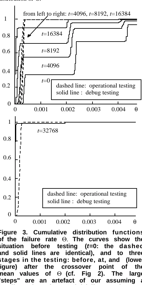
Figure 3. Cumulative distribution functions of the failure rate Θ. The curves show the situation before testing (t=0: the dashed and solid lines are identical), and to three stages in the testing: before, at, and (lower figure) after the crossover point of the mean values of Θ (cf. Fig 2). The large "steps" are an artefact of our assuming a small number of potential failure regions.
Figure 3 shows the cumulative probability distributions P(Θo≤θ) and P(Θd≤θ), for t=0 (before testing), t=8192
(when operational testing delivers a better expected failure rate), t=16384 (when the two approaches deliver the same expected failure rate) and t=32768 (when debug testing delivers a better expected failure rate).
As shown in Fig. 3, P(Θo≤4 10 -4
[image:7.595.57.280.481.620.2]7
number of
tests E(Θo) E(Θd) P(worse thanΘo|≥3 10-4):
E(Θd(t=16384) )
P(Θd ≥3 10-4): worse than E(Θd(t=16384) )
P(Θo≥2 10-3) (at least 1 large failure region in the program)
P(Θd ≥2 10-3) (at least 1 large failure region in the program)
t=0 2.36 10-3 2.36 10-3 0.985 0.985 0.651 0.651
t=8192 3.06 10-4 7.82 10-4 0.473 0.286 7.556 10-8 0.286
t=16384 2.59 10-4 2.59 10-4 0.116 0.105 <<10 -15 0.105
[image:8.595.65.524.82.207.2]t=32768 1.86 10-4 2.85 10-5 0.0025 0.012 ~0 0.012
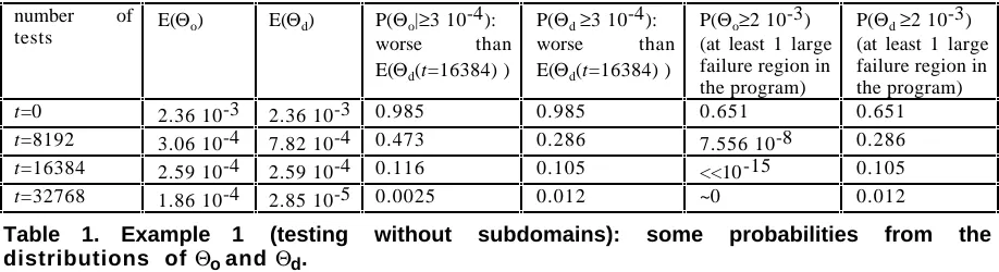
Table 1. Example 1 (testing without subdomains): some probabilities from the distributions of Θo and Θd.
failure rate possible if no large failure region is present, given by n2=20 "small" failure regions, each contributing a failure rate q2=2 10
-5
). On the other hand, "debug-tested" programs have a non-negligible probability of containing some "large" failure region, even after their average failure rate has dropped below that achieved by operational testing.
Some interesting facts are summarized in Table 1:
• "on average", operational testing is better than debug testing (E(Θo)<E(Θd)) for t<16384; for t>16384, debug
testing is better (E(Θo)>E(Θd));
• for t=16384, both methods deliver a mean failure rate which is about ten times better than the mean before testing. However, debug testing leaves a large amount of variation among programs in the population, while operational testing almost eliminates this variation. About 10% of the "debug-tested" programs still have one or more "large" failure regions (i.e., a failure rate comparable to the mean before testing) while this percentage is negligible for operational testing;
• for t=32768, E(Θd) is 84 times smaller than the mean
before testing and 7 times smaller than E(Θo). Still,
about 1.2% of "debug-tested" programs have a failure rate that is worse than the mean before testing; this percentage is negligible for operational testing.
We also observed that operational testing achieves a consistently narrower distribution of the failure rate than debug testing. For instance, the probability of a failure rate worse than twice the mean failure rate is always higher with debug testing than with operational testing.
4. Testing with subdomains
We now consider the case in which the debugger subdivides the input domain into sets (subdomains), according to some similarity criterion. With the ideal choice of subdomains, each subdomain is such that either the program fails on all its points or on none of them (homogeneous subdomains [2]). If the debugger has the ability to produce homogeneous subdomains, it is enough to test one representative input from each subdomain.
Here, we assume this "ideal" debugger, and show that, even under this assumption, there may be cases in which operational testing is preferable to debug testing.
The "ideal" debugger guesses exactly where all the potential failure regions are. He/she defines homogeneous
subdomains so that each coincides with a potential failure region, plus a subdomain for those input points, if any, that cannot belong to any failure region (due to our assumption of non-overlapping failure regions, these subdomains form a partition over the input space). He/she then chooses each successive test from a new (randomly and uniformly chosen) subdomain in this set of ni
i=1 N ∑
"interesting" subdomains.
This models a debugger with perfect information about where the failure regions may be, but no information about their sizes (qi) and about their probabilities (pi) of being actually present in a given program.
Obviously, if any program from our population is subjected to a number of tests t≥ ni
i=1 N
∑ , all its failure
regions will be removed. Besides, if 1 nj j=1
N
∑ >qi for all i,
debug testing has a higher probability than operational testing of finding any given failure region: it thus delivers stochastically better reliability, for every program from the population. We are more interested in the other cases, in which the number of potential failure regions, and thus the number of subdomains, is very high, so that:
a) it is not possible to test every subdomain (t< ni i=1
N ∑ ), b) there are some large failure regions for which, at least
at an early stage, operational testing is more appropriate than debug testing ( i.e. for some j, qj>
1 ni ∑ ).
Conditions a) and b) seem realistic in most practical situations.
4.1. Comparing the expected values of the failure rate after testing
The probability that a potential failure region of class i is actually present, and remains in a debug-tested program
after t tests, is the product, pi⋅ 1−
t ni ∑
. After t tests:
E(Θd)= 1−
t
i n
∑
∑ni⋅pi⋅qi, for debug testing, vs. :
E(Θo)= ni⋅pi⋅qi⋅ t (1−q )i
∑ for operational testing.
0 20 40
0 0.02 0.04 0.06 0.08 0.1
t
E(Θd) E(Θo)
dashed line: operational testing solid line : debug testing
Figure 4. Subdomain testing: evolution of E (Θo) and E(Θd) as t increases.
E(Θd) decreases linearly to zero as t increases to ∑ni;
instead, E(Θo)>0 for every t. Thus, debug testing
guarantees a better expected value, if enough tests are run. On the other hand, operational testing may give a better expected Θ in the early stages of testing, thanks to its ability to find the large failure regions first.
Example 2: We choose N=2, n1=10, n2=42, p1=0.1, p2=0.5, q1=8 10
-2
, q2=10
-3
. After 52 tests, the debugger has removed all the failure regions from any program from the population, thus it is interesting to compare the two methods for t<52. Debug testing and operational testing produce the same average failure rate for t=40.
The probability of hitting a failure region at the first test is 0.1 for operational testing vs. 0.423 for debug testing. However, operational testing is more than three times more effective (at the first test) than debug testing from the reliability point of view, i.e. 1
i n
∑ =1.9 10-2 and i
n⋅pi⋅ i 2 q
∑ i n⋅pi⋅qi
∑ =6.4 10-2. Figure 4 compares E(Θo) and E(Θd)
as functions of t. One can see that operational testing delivers a better expected failure rate for t<40.
4.2. The probability distribution of the failure rate after testing
We now study the distributions of Θo and Θd in this
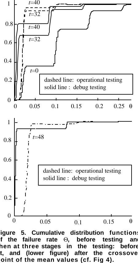
example. Figure 5 shows the cumulative probability distributions P(Θo≤θ) and P(Θd≤θ), as functions of θ, for
t=0 (before testing), t=32 (when operational testing
delivers a better expected failure rate), t=40 (when the two approaches deliver the same expected failure rate) and t=48 (when debug testing delivers a better expected failure rate). The interpretation of these graphs is exactly the same as for Figure 3. P(Θ≤8 10-2) represents the probability that a randomly selected program contains at most 1 large failure region, P(Θ≤1.6 10-1) is the probability that it contains at most two large failure regions, and so on. The considerations we can make about figure 5 are very similar to those made in Section 3 about operational testing vs. debug testing without subdomains.
0 0.2 0.4 0.6 0.8 1
0 0.05 0.1 0.15 0.2 0.25 θ
t=40
t=0 t=32
t=32 t=40
dashed line: operational testing solid line : debug testing
0 0.2 0.4 0.6 0.8 1
0 0.05 0.1 0.15 θ
t=48
[image:9.595.56.286.135.374.2]dashed line: operational testing solid line : debug testing
Figure 5. Cumulative distribution functions of the failure rate Θ, before testing and then at three stages in the testing: before, at, and (lower figure) after the crossover point of the mean values (cf. Fig 4).
Some interesting facts are summarized in Table 2:
• for t<40, E(Θo)<E(Θd); for t>40, E(Θo)>E(Θd).
[image:9.595.314.539.208.636.2]9
"large" failure region (so their failure rate is comparable to the mean before testing), and 2% at least two "large" failure regions, while these percentages are respectively 3.5% and 0.042% for operational testing.
• for t=48, the expected failure rate obtained with debug testing is much smaller than with operational testing. Nevertheless, about 6 % of the "debug-tested" programs contain at least one large failure region (vs. only 1.9% for operational testing).
As for Example 1, the probability of a failure rate worse than twice the mean failure rate is constantly higher with debug testing than with operational testing.
5. Considerations on the distribution
of the failure rate before testing
As we said in section 1, one source of variation among test results is the variation among programs before testing.
A testing method may be very good in improving the reliability of some programs and almost ineffective for others. In our examples, we assumed the presence of each failure region to be independent of the presence of any other failure region. The number of failure regions of any given class thus has a binomial distribution.
In this section we address two possible doubts:
1. do we need explicitly to model the variation among programs? For instance, could we simply assume that the program under test is the "average" program in the population of interest?
2. how would our observations change if the variation of failure rates before testing were greater (or smaller) than in our model? For instance, we could have positive correlation among the presence of certain failure regions
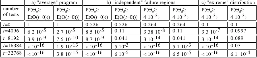
(i.e. a programmer who makes a certain mistake is also likely to make some other mistakes of the same type). We refer to Example 1 (Section 3), and consider three different scenarios, with identical expected failure rates after any number t of tests, but characterized by increasingly varied populations of programs:
a) all programs tested are identical to the "average" program from the distribution in Example 1, with exactly ni• pi failure regions from each class i: there is no variation (before testing) among programs in the population;
b) our assumptions in Section 3 are true: the number of failure regions in each class has binomial distribution; c) each program either contains 10 "large" failure regions
(with probability 0.1) or none (with probability 0.9); this is an extreme case in which there is the greatest variation possible over the population of programs. Table 3 shows some meaningful steps in the evolution of the reliability of randomly chosen programs under the three different assumptions. The testing regimes compared are operational testing and debug testing without subdomains (as modelled in Section 3). Clearly, the distribution of Θ before testing greatly affects the distribution after testing. The average results are the same for all distributions of programs; the interesting data in the table are the probabilities of a high failure rate after t tests. Two phenomena are of interest: how the chosen distributions of programs affects these probabilities, for a given testing method, and how it affects the relative advantage of one method over the other. For instance, we observe that operational testing achieves very similar results for the three distributions, and its advantage over debug testing increases from case a) to case c). For debug testing, the inadequacy in improving the worse programs in the population gets worse from case a) to case c).
number of
tests E(Θo) E(Θd) P(at least 1 largeΘo≥8 10-2):
failure region left
P(Θd≥8 10-2) : at least 1 large failure region left
P(Θo≥1.6 10-1): at least 2 large failure regions
P(Θd≥1.6 10-1): at least 2 large failure regions
t=0 0.1 0.1 0.65 0.65 0.26 0.26
t=32 2.6 10-2 3.9 10-2 6.8 10-2 3.3 10-1 1.62 10-3 5.3 10-2
t=40 2.3 10-2 2.3 10-2 3.5 10-2 2.1 10-1 4.2 10-4 2 10-2
t=48 2.1 10-2 7.8 10-3 1.9 10-2 6.1 10-2 1 10-4 2 10-3
Table 2. Example 2 (testing with "ideal" subdomains): some probabilities from the distributions of Θo and Θd.
a) "average" program b) "independent" failure regions c) "extreme" distribution
number
of tests P(Θo≥
E(Θ(t=0)))
P(Θd≥
Ε(Θ(t=0)))
P(Θo≥ E(Θ(t=0)))
P(Θd≥
Ε(Θ(t=0)))
P(Θo≥ 4 10-3)
P(Θd≥ 4 10-3)
P(Θo≥ 4 10-3)
P(Θd≥ 4 10-3)
t=0 1 1 0.526 0.526 0.264 0.264 0.1 0.1
t=4096 6.2 10-5 2.7 10-5 8.5 10-5 0.11 3.38 10-8 0.11 3.3 10-7 0.0997
t=8192 3.9 10-9 7.5 10-10 8.7 10-9 0.041 3 10-14 0.041 3 10-14 0.089
t=16384 < 10-16 1.9 10-13 < 10-16 5 10-3 < 10-16 5.1 10-3 < 10-16 0.03
[image:10.595.68.520.598.700.2]t=32768 < 10-16 3.8 10-15 < 10-16 6 10-5 < 10-16 6.5 10-5 < 10-16 6.1 10-4
6. Conclusions
We have studied, under various assumptions, the effectiveness of testing in improving program reliability. While previous studies assumed a known program with known faults, we studied the reliability that can be achieved given that the program under test is only known in a probabilistic sense, as being the product of a known process.
We only showed the behaviors of a few examples, so any generalisation from these examples must be taken as a simple conjecture. However, these conjectures seem correct on the basis of physical intuition, and thus deserve further investigation:
- the variation in the results of a production process implies variation in the results of testing as well, and project decisions must take this into account;
- operational testing may offer great advantages if the main concern is predictability of the quality of delivered programs, by being more efficient at pruning the "tail" of extremely unreliable programs;
- operational testing offers these advantages even in many situations in which other testing methods provide better reliability on average.
Which method is actually most effective in a given practical situation cannot be decided by mathematical analysis only: empirical measurements are needed to decide which model assumptions are verified in that situation, and to estimate the values of the parameters. However, for operational testing not to have the above advantages it seems necessary that the chosen "debug testing" method be consistently superior to operational testing for every possible failure region.
We have ignored the cost of tests and the cost of fixes: we only compared the reliability achieved by different methods after a given number of tests (and the fixes that these tests may have prompted). Considering such costs, in situations where budget is the main limiting factor, would improve the position of those methods that can be more completely automated, and those that require fixing fewer faults to achieve a given reliability. Both factors seem to further favor operational testing.
We have also shown that under this model, as under previous ones, the best choice of testing methods should be expected to vary not only between different projects, but also during the evolution of a single program.
A necessary next step is to transform our conjectures into theorems that are true under usefully wide classes of hypotheses, or to disprove them. An immediate use of our examples is in avoiding wrong "common sense" judgements by providing counterexamples. Practical applications of these more general theorems (which we hope to produce) to project management must depend on verifying which hypotheses (on the distributions of failure rates from individual failure regions, and on the strengths and weaknesses of human testers) apply in different industrial environments and project phases. Our models
point at the kind of data to be collected and hypotheses to be tested, and may support statistical inference to correctly estimate the model parameters from the data.
Acknowledgements
This research was funded in part by the European Commission via the "OLOS" research network and the ESPRIT Long Term Research Project 20072 "DeVa", and by the U.K. Engineering and Physical Sciences Research Council within project DISCS (grant GR/L07673). The authors are indebted to David Wright for his advice and comments.
References
[1] J. Duran and S. Ntafos, "An evaluation of random testing", IEEE TSE, 10, pp. 438-444, 1984.
[2] D. Hamlet and R. Taylor, "Partition testing does not inspire confidence", IEEE TSE, 16, pp. 1402-1411, 1990.
[3] B. Jeng and E. J. Weyuker, "Analyzing partition testing strategies", IEEE TSE, 17, pp. 703-711, 1991.
[4] T. Y. Chen and Y. T. Yu, "On the expected number of failures detected by subdomain testing and random testing", 22, pp. 109-119, 1996.
[5] W. E. Wong, J. R. Horgan, S. London and A. P. Mathur, "Effect of test set size and block coverage on the fault detection effectiveness", SERC Technical Report SERC-TR-153-P, 1994.
[6] P. G. Frankl and S. N. Weiss, "An experimental comparison of the effectiveness of branch testing and data flow testing", IEEE TSE, 19, pp. 774-787, 1993. [7] P. Frankl and E. J. Weyuker, "A formal analysis of the
fault-detecting ability of testing methods", IEEE TSE, 19, pp. 962-975, 1993.
[8] P. Frankl, D. Hamlet, B. Littlewood and L. Strigini, "Choosing a Testing Method to Deliver Reliability", in Proc. 19th International Conference on Software Engineering (ICSE'97), 1997, pp. 68-78.
[9] P. Frankl, D. Hamlet, B. Littlewood and L. Strigini, "Evaluating testing methods by delivered reliability", IEEE TSE, to appear, 1998.
[10] N. Li and Y. K. Malaiya, "On Input Profile Selection for Software Testing", in Proc. 5th Intl Symposium on Software Reliability Engineering, ISSRE'94, 1994, pp. 196-205.