City, University of London Institutional Repository
Citation:
Kaishev, V. K., Dimitrova, D. S., Haberman, S. and Verrall, R. J. (2006). Geometrically designed, variable knot regression splines: variation diminish optimality of knots (Statistical Research Paper No. 29). London, UK: Faculty of Actuarial Science & Insurance, City University London.This is the unspecified version of the paper.
This version of the publication may differ from the final published
version.
Permanent repository link:
http://openaccess.city.ac.uk/2373/Link to published version:
Statistical Research Paper No. 29Copyright and reuse: City Research Online aims to make research
outputs of City, University of London available to a wider audience.
Copyright and Moral Rights remain with the author(s) and/or copyright
holders. URLs from City Research Online may be freely distributed and
linked to.
Faculty of Actuarial
Science
and
Insurance
Geometrically Designed,
Variable Knot Regression
Splines: Variation Diminishing
Optimality of Knots.
Vladimir K. Kaishev, Dimitrina S. Dimitrova,
Steven Haberman and Richard Verrall.
Statistical
Research Paper No. 29
October 2006
ISBN 1-905752-03-2
Cass Business School
106 Bunhill Row
London EC1Y 8TZ
knot regression splines: Variation
diminishing optimality of knots
by
Vladimir K. Kaishev
*, Dimitrina S. Dimitrova, Steven Haberman
and Richard Verrall
Cass Business School, City University, London
Summary
A new method for Computer Aided Geometric Design of variable knot regression splines, named GeDS, has recently been introduced by Kaishev et al. (2006). The method utilizes the close geometric relationship between a spline regression function and its control polygon, with vertices whose y-coordinates are the regression coefficients and whose x-coordinates are certain averages of the knots, known as the Greville sites. The method involves two stages, A and B. In stage A, a linear LS spline fit to the data is constructed, and viewed as the initial position of the control polygon of a higher order (n>2 ) smooth spline curve. In stage B, the optimal set of knots of this higher order spline curve is found, so that its control polygon is as close to the initial polygon of stage A as possible, and finally the LS estimates of the regression coefficients of this curve are found. In Kaishev et al. (2006) the implementation of stage A has been thoroughly addressed and the pointwise asymptotic properties of the GeD spline estimator have been explored and used to construct asymptotic confidence intervals.
In this paper, the focus of the attention is at giving further insight into the optimality properties of the knots of the higher order spline curve, obtained in stage B so that it is nearly a variation diminishing (shape preserving) spline approximation to the linear fit of stage A. Error bounds for this approximation are derived. Extensive numerical examples are provided, illustrating the performance of GeDS and the quality of the resulting LS spline fits. The GeDS estimator is compared with other existing variable knot spline methods and smoothing techniques and is shown to perform very well, producing nearly optimal spline regression models. It is fast and numerically efficient, since no deterministic or stochastic knot insertion/deletion and relocation search strategies are involved.
Keywords: spline regression, B-splines, Greville abscissae, variable knot splines, control polygon, asymp-totic confidence interval
1. Introduction.
Consider the problem of nonparametric spline regression estimation in which, a response variable y is related to an independent variable xœ@a,bD, through the functional relation-ship
(1) y= fHxL+ e,
where e is a random error variable with zero mean and fHÿL is an unknown function, approximated with a n-th order (degree n-1) polynomial spline fHtk,n;xL. The latter is
defined on the set of knots
(2)
tk,n=8t1= ...=tn=a<tn+1<...<tn+k<tn+k+1=b= ...=t2n+k<
as
(3) fHtk,n;xL=q'NnHxL=⁄i=1
p q
iNi,nHxL,
where q=Hq1, ..., qpL' is the vector of regression coefficients and NnHxL=HN1,nHxL, ..., Np,nHxLL', p= n+k, are the B-splines of order n. B-splines are
defined on tk,n through the Mansfield-De Boor-Cox recurrence relation
Ni,1HtL=9 1 0
if
ti§t<ti+1 otherwise ,
(4) Ni,nHtL=ÅÅÅÅÅÅÅÅÅÅÅÅÅÅÅÅÅÅt t-ti
i+n-1-ti Ni,n-1HtL+ ti+n-t
ÅÅÅÅÅÅÅÅÅÅÅÅÅÅÅÅÅÅt
i+n-ti+1 Ni+1,n-1HtL.
from which it can be seen that Ni,nHtL=0 for t–@ti,ti+nD. In the sequel, where necessary,
we will emphasize the dependence of the spline regression fHtk,n; xL on q by using the
alternative notation fHtk,n,q;xL. The nonparametric spline regression problem is then to
estimate the degree of the spline, n, the number of the knots, k, their location and the regression coefficients q, based on a sample of observations 8yi<iN=1 at some design points 8xi<iN=1.
Several different nonparametric spline approximation methods can be outlined. Under the direct approach, n and k are considered fixed (but unknown), and the knots tk,n are
assumed to be unknown parameters which have to be estimated by solving a non-linear least squares optimization problem (see DeBoor and Rice (1968), Jupp (1978), Hu (1993) and Lindstrom (1999)), based on the sample 8yi,xi<iN=1. There are a number of difficulties related to this approach which have been pointed out by Jupp (1978) and Lindstrom (1999). All these difficulties have been shortly summarized by Carl DeBoor , who writes, "...it is essentially impossible to characterize a best approximation, that is to give a computationally useful criteria by which a best approximation can be recognized and distinguished from other approximations" (see DeBoor 2001, page 239).
Friedman and Silverman (1989), Friedman (1991), Stone et al. (1997) and more recently by Zhou and Shen (2001), where some drawbacks of this approach have been pointed out.
Another group of works applies reversible jump Markov chain Monte Carlo (RJMCMC) based methods to develop Bayesian adaptive splines, such as those of Smith and Kohn (1996), Denison et al. (1998) and Biller (2000), in the context of generalized linear models. These procedures simulate tens of thousands of spline models, which are then averaged point-wise, to produce a resulting estimate of f. These methods are thus associ-ated with a high computational cost and the inconvenience of having the resulting model in a non-explicit form. A stochastic optimization algorithm for free-knot splines, called adaptive genetic splines (AGS), was recently proposed by Pittman (2002) but the related computational cost is also a concern, as noted by the author.
Smoothing spline fitting methods, involving a smoothing penalty in the objective func-tion have also been proposed in the statistical literature. We will menfunc-tion here the hybrid adaptive splines (HAS) of Luo and Wahba (1997) and the penalized splines, considered by Eubank (1988), Wahba (1990), Marx and Eilers (1996), Rupert and Carroll (2000), Rupert (2002) and Wood (2003). Some asymptotic results, related to spline regression estimation are due to Agarwal and Studden (1980) and more recently to Huang (2003), where other references can be found.
Recently, a geometrically motivated method of variable knot spline regression estima-tion, which is new and very different from the existing methods, has been proposed by Kaishev et al. (2006). It is based on the so called Schoenberg's variation diminishing spline (VDS) approximation scheme, applied to the knot selection problem. The VDS approximation has some nice geometric properties such as shape preservation, which have made it fundamental in developing the Computer Aided Geometric Design (CAGD) methodology. These properties have been essential in developing the new variable-knot spline regression estimation method of Kaishev et al. (2006), called Geo-metrically Designed (GeD) spline estimation or simply GeDS. The latter produces a spline fit which is a least squares estimate with respect to its regression coefficients, but whose knots are placed in such a way that the fit has also the characteristics of a VDS approximation.
The purpose of this paper is to give some further insight into the optimality properties of the knot placement proposed by Kaishev et al. (2006), to explore further the pointwise asymptotic properties and related confidence intervals and the numerical performance of the proposed GeD spline estimator and compare it with other existing spline estimators.
the fact that a spline regression function has a control polygon, and by manipulating the position of its vertexes it is possible to estimate the location of the knots and the regres-sion coefficients. Section 3 gives a brief outline of the two stages A and B of the GeD spline regression estimation method and provides further comments on the solution of the constrained minimization problem of stage B. The optimality properties of the knots of the higher order spline regression model, obtained in stage B are discussed and explored in Section 4. These knots are such that their related higher order spline curve is nearly a variation diminishing approximation to the control polygon of stage A. Bounds for its deviation from the variation diminishing approximation are established by Theo-rem 1 and its Corollaries 1.1 and 1.2, in Section 4. In Section 4.1 the averaging knot location method, proposed in Kaishev et al. (2006), which gives good approximate values of the optimal knots of stage B, is revisited. It is shown that it leads to bounds, given by Theorem 2 and Corollaries 2.1 and 2.2, which are sharper than those estab-lished by Theorem 1 and its corollaries. Section 5 gives a summary of the pointwise asymptotic properties of GeDS, including the construction of asymptotic confidence intervals. In Section 6, six numerical examples are presented, on which the GeDS method is thoroughly tested and compared with other existing spline approximation methods. Proofs of the theorems and their corollaries are given in the Appendix.
2. Geometric interpretation of the spline regression estimation.
Since our main purpose in this paper is to explore the optimality properties of the knots, placed according to the GeD spline regression method of Kaishev et al. (2006), we will first review its basic characteristics and give a short description of it. The method is motivated by the observation that the spline regression fHtk,n,q;xL introduced in (3) as
a function of an independent variable xœ@a,bD can be viewed as a special case of a parametric spline curve. A parametric spline curve QHtL is given coordinate-wise as
QHtL=8xHtL, yHtL<=8⁄ip=1xiNi,nHtL,⁄i=1
p q
iNi,nHtL<,
where t is a parameter, and xHtL and yHtL are spline functions, defined on one and the same set of knots tk,n. In view of the identity
(5) xHtL=⁄ip=1xi*Ni,nHtL=t,
known as linear precision property, with xi* defined as the averages
(6)
xi*=Ht
i+1+...+ti+n-1L ê Hn-1L, i=1, ..., p.
of the n-1 consecutive knots ti+1, ..., ti+n-1, we can express a spline regression func-tion fHtk,n,q;tL, tœ @a,bD, as
(7)
Q*HtL=8t, fHtk,n,q;tL<=8⁄i=1
p x
i*Ni,nHtL,⁄i=1
p q
i.e., fHtk,n,q;xL, xœ @a,bD can be equivalently expressed in a parametric form as a
spline regression curve Q*HxL.
The values xi* given by (6) are known as the Greville abscissae. We will alternatively use the notation x*Htk,nL, to indicate the dependence of the set of Greville sites
x* =8x1*, ...,x
p
*<ªx*Ht
k,nL on the knots tk,n.
Based on this parametric interpretation, it has been noted by Kaishev et al. (2006) that
Q*HtL can be characterized by a polygon CQ*, which is closely related to it and is called
its control polygon. The vertices of the control polygon, called control points, are the points, ci, whose x- and y-coordinates are correspondingly the Greville sites xi* and the B-spline regression coefficients qi, i.e., ci=Hxi*,qiL, i=1, ..., p. This close relationship
between the spline regression curve and its control points is discussed and illustrated in Section 2.2. Due to the partition of unity property of B-splines,
⁄i=j-n+1
j
Ni,nHtL=1, for any tœ@tj,tj+1L, j=n, ... , n+k,
every point of the spline regression curve Q*HtL of order n is a convex combination of n control points ci, i.e., Q*HtL=⁄i=j
n+j-1
ciNi,nHtL for tœ@tn+j-1,tn+jD, j=1, ...,k+1. This
means that each polynomial segment of Q*HtL lies within the convex hull of the n control points, cj, ..., cj+n-1, j=1, ...,k+1, defining it (see Section 2.2). The convex hull of
cj, ..., cj+n-1 is the smallest convex polygon, enclosing these points.
In fact, the control polygon CQ* with vertices ci=Hxi*,qiL is itself a linear spline
func-tion, and hence can be expressed as
(8)
CQ*HtL=8⁄i=1
p x i
*N
i,2HtL,⁄i=1
p q
iNi,2HtL<=8t,⁄i=1
p q
iNi,2HtL<ª⁄i=1
p q
iNi,2HtL .
In (8), ⁄ip=1xi*Ni,2HtL=t since Ni,2HtL are defined over the knots tp-2,2, where t1ª x1*,
tp+2ª xp* and ti+1ª xi*, i=1, ..., p and the linear precision property (5) applies.
Since Q*HtL is a convex combination of its control points, its graph lies within the con-vex hull of its control polygon CQ*. Moreover, as has been pointed out by Kaishev et al.
(2006), the spline regression curve Q*HtL lies close to its control polygon CQ* also
because Q*HtL is the shape preserving, Schoenberg's VDS approximation of CQ*. Since
the concept of VDS approximation to a function g, defined on @a,bD is central in deriv-ing the optimality properties of the GeDS knots, we will recall its definition and basic properties.
2.1. Schoenberg's variation diminishing spline approximation.
Given a set of knots tk,n, a function g, defined on @a,bD, can be approximated by the
spline function
(9) V@gDHxL=⁄ip=1gHxi*LNi,nHxL,
The spline V@gD is known as the Schoenberg's variation diminishing spline approxima-tion of order n to g, on the set of knots tk,n. It is constructed by simply evaluating g at
the Greville sites (6) and taking the values gHxi*L as the B-spline coefficients. The varia-tion diminishing character of (9) is due to the fact that V@gD crosses any straight line at most as many times as does the function g itself. The latter suggests the following proper-ties, which justify the importance of the VDS approximation in CAGD applications.
Property 1 (Shape preservation). The VDS approximation is shape preserving since it preserves the shape of the function g it approximates. More precisely, if g is positive, then V@gD is also positive; if g is monotone, then V@gD is also monotone; and if g is convex, V@gD is also convex.
Property 2 (Reproduction of straight lines). The VDS approximation reproduces any straight line lHtL, tœ@a,bD. In particular, V@tD=t, which follows from the linear preci-sion property (5).
We will see in Section 3 that the way knots are found in stage B allows the GeD spline approximation to incorporate the features of a VDS approximation. Properties 1 and 2 are also used in the next section to show the closeness of a spline regression curve to its control polygon, a fact essentially used to motivate the GeDS estimation method. Fur-ther details on geometric modelling with splines and related results are to be found in Farin (2002).
2.2. The spline regression curve and its control points.
Since the graph of Q*HtL lies within the convex hull of its control polygon CQ* and since
Q*HtL is the shape preserving, Schoenberg's VDS approximation of CQ*, (as follows
from Property 1, Section 2.1, taking gªCQ*), the spline regression curve Q*HtL closely
follows the shape of CQ*. We illustrate the shape preserving and convex hull properties
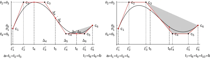
in Fig. 1 where functional spline regression curves, Q*HtL, of order n=3 and n=4 and their control polygons, CQ*, are plotted. The grey areas in Fig. 1 are the two convex
hulls, formed by c4,c5,c6 for the quadratic curve (left panel) and c3,c4,c5,c6 for the cubic curve (right panel) within which the corresponding segment of Q*HtL for tœ@t6,t7D lie.
Note that a linear spline curve QHtL (order n=2) coincides with its control polygon CQ.
In the quadratic case Hn=3L, the spline curve QHtL, evaluated at the knots t3,t4, ..., tk+4, interpolates CQ and is tangential to each of its segments, ci,ci+1, dividing it in a propor-tion Hti+2-ti+1L:Hti+3-ti+2L, i=1, ..., k+2. This is illustrated in the left panel of Fig. 1, for the case of k=3, where Dj=tj+1-tj, j=3, ...k+3. In the cubic case Hn=4L,
the spline curve evaluated at a knot, QHti+3L is somewhere within the triangle of points
but it still remains within the convex hull of CQ. This suggests that a quadratic B-spline
curve is very well suited as a compromise between smoothness and shape preservation.
x1*
a=t1=t2=t3 x2 * x 3 * x 4 * x 5 *
t4 t5 t6 x6*
t7=t8=t9=b q1
q2=q3
q4=q5 q6
D4 D5 D6
c1
c2 c3
c4 c5
c6
D
4
:D
5
D5:D6
x1*
a=t1=t2=t3=t4 x2 * x 3 * x 4 * x 5 *
t5 t6 x6*
t7=t8=t9=t10=b q1
q2=q3
q4=q5 q6
c1
c2 c3
[image:10.595.78.505.127.248.2]c4 c5 c6
Fig. 1. Quadratic (left panel) and cubic (right panel) functional spline curves Q*HtL and their control
polygons CQ*.
The close geometric relationship between the spline regression curve
Q*HxL=8x, fHtk,n,q;xL<, xœ@a,bD, and its control polygon CfHtk,n,q;xL, is the foundation
of the GeDS method, proposed in Kaishev et al. (2006). Here, we briefly summarize the logic behind this new geometrically motivated estimation approach. Since the x -coordi-nates of the vertices ci=Hxi*,qiL, i=1, ...p, of CfHtk,n,q;xL are the Greville sites, xi
*,
obtained from tk,n, and the y-coordinates are the regression coefficients qi, estimation of tk,n and q, based on 8yi, xi<iN=1, affects the geometric position of the control polygon
CfHtk,n,q;xL. On the other hand, due to the shape preserving and convex hull properties, CfHtk,n,q;xL defines the location and the shape of the spline curve fHtk,n,q;xL. So,
manipu-lating the vertices ci of CfHtk,n,q;xL, affects the knots tk,n, through (6), and the regression
coefficients q, which affects the position of the regression curve fHtk,n,q;xL itself. The
latter conclusion has motivated the construction, in stage A of GeDS, of a control poly-gon as a linear least squares spline fit to the data, whose knots determine the knots tk,n,
and whose B-spline coefficients, are viewed as initial estimate of q, which is improved further in stage B (see Section 3). This is the basis of the approach which has been used by Kaishev et al. (2006) in constructing GeD variable knot spline approximation to the unknown function f in (1). The GeDS method is briefly described in the next Section 3.
3. The GeD spline regression estimation method.
a smooth, higher order LS spline fit, obtained in stage B. In stage B a smooth LS spline fit to the data which closely follows the shape of the piece-wise linear fit from stage A is constructed. To achieve this, the knots of the latter linear fit are used to locate the knots of a functional spline curve, which is not an LS fit to the data, but which does follow the shape of the linear fit from stage A in the sense that it is nearly a VDS approximation to it. Then, its B-spline coefficients are adjusted in order to ensure that it is an LS fit. In Kaishev et al. (2006) stages A and B have been given the following more formal defini-tion as certain optimizadefini-tion problems.
Stage A. Fix the order n=2. Starting from a straight line fit and adding one knot at a time, find the least squares linear spline fit f`Hdl,2,a`;xL=⁄i=1
p a`
iNi,2HxL with a number of internal knots l, number of B-splines p=l+2 and with a set of knots
dl,2=8d1= d2< d3<...< dl+2< dl+3= dl+4<, such that the ratio of the residual sums of squares
RSSHl+qL êRSSHlL=‚
j=1
N
Hyj- f
`
Hdl+q,2;xjLL
2
í ‚Nj=1 Hyj- f
`
Hdl,2;xjLL
2¥ a exit
where aexit is a certain threshold level. This means that f
`
Hdl,2,a`;xL could not be signifi-cantly improved if q more knots are added, q¥1, and therefore f`Hdl,2,a`;xL adequately reproduces the "shape" of the unknown underlying function f. The resulting linear LS spline fit f`Hdl,2,a`;xL is viewed as a control polygon with vertices Hxi,a`iL, i=1, ..., p,
where xiª di+1, i=1, ..., p. The fit f
`
Hdl,2,a`;xL is constructed following an algorithm described in Kaishev et al. (2006).
Stage B. For each of the values of n=3, ..., nmax, find the optimal position of the knots
t
é
l-Hn-2L,n, as a solution of the constrained minimization problem
(10) min
tl-Hn-2L,n,
xi+1<ti+n<xi+n-1,
i=1,...,k
±f`Hdl,2,a`;xL-CfHtl-Hn-2L,n,a`;xLµ,
where ∞g¥:=maxa§x§b »gHxL » is the uniform (L¶) norm of a function gHxL, and xi,
i=1, ..., p are the x-coordinates of the vertices of the control polygon f`Hdl,2,a`;xL obtained in stage A. In fact, minimization in (10) is over all polygons CfHtl-Hn-2L,n,a`;xL
which have verticesHxi*,a`iL, with x-coordinates which are the Greville sites x*Htl-Hn-2L,nL,
and y-coordinates, coincident with the y-coordinates a`i of the vertices of the polygon
f`Hdl,2,a`;xL.
Our purpose here will be to comment on the possibility of solving problem (10) and to give some further insight into the optimality of the knots tél-Hn-2L,n obtained as its
solu-tion. In order to do so, we first note that the two polygons f`Hdl,2,a`;xL and CfHtl-Hn-2L,n,a`;xL
have the same number of vertices p=l+2, since the number of internal knots in
tl-Hn-2L,n is l-Hn-2L. Ideally, it will be desirable to find an optimal set of knots t
é
l-Hn-2L,n
for which the minimum in (10) is zero, i.e., CfHté
l-Hn-2L,n,a`;xL ª f
`
one would require that tél-Hn-2L,n be such that fHt
é
l-Hn-2L,n,a`;xL becomes the VDS
approxi-mation to f`Hdl,2,a`;xL, or equivalently f`Hdl,2,a`;xL becomes the control polygon of the spline function fHtél-Hn-2L,n,a`;xL. In this way the knots t
é
l-Hn-2L,n match best the
geometri-cal form of f`Hdl,2,a`;xL and as a consequence, the geometrical form of the data.
Since the two polygons in (10), CfHtl-Hn-2L,n,a`;xL and f`Hdl,2,a`; xL, have the same y -coordi-nates a`, they will coincide if their x-coordinates coincide, i.e., if xi*ª xi, i=1, ..., p.
The latter would be fulfilled if, for given Greville sites xi*= xi, it would be possible to
solve the system (6) with respect to tl-Hn-2L,n.
However, to find tél-Hn-2L,n, so that equations (6) are fulfilled with respect to xi,
i=1, ..., p is, in general, impossible. This is easily seen from the fact that (6) represents an over-determined system of equations, with constraints on the knots, given by the definition (2) of tl-Hn-2L,n. Since x1=a and xp=b, the system (6) contains l equations
and l-Hn-2L ordered, unknown knots, Hn>2L. Thus, it is in general impossible to place the knots tél-Hn-2L,n in such a way that CfHétl-Hn-2L,n,a`;xLª f
`
Hdl,2,a`;xL, i.e., xi* ª xi, for
any fixed set 8xi<, i=1, ..., p. Instead, what is achieved by solving (10) is that CfHté
l-Hn-2L,n,a`;xL gets as close to f
`
Hdl,2,a`;xL as possible, simultaneously with x* getting as close to x as possible. Note that since we view the x-coordinates of the vertices of f`Hdl,2,a`;xL, xi, as Greville sites of a higher order spline curve fHtl-Hn-2L,n, a`;xL, the
constraints xi+1< ti+n< xi+n-1, i=1, ..., k in (10), follow from (6).
Since the resulting curve fHtél-Hn-2L,n,a`;xL is the variation diminishing (i.e. shape
preserv-ing) spline approximation of its control polygon CfHté
l-Hn-2L,n,a`;xL (see Section 2), and since
the latter is the best uniform (L¶) approximation of f`Hdl,2,a`;xL in (10),
fHétl-Hn-2L,n,a`;xL will closely follow the shape of f
`
Hdl,2,a`;xL. The fact that
fHétl-Hn-2L,n,a`;xL is nearly a VDS approximation to f
`
Hdl,2,a`;xL is proved in Section 4. However, as has been noted in Kaishev et al. (2006), fHtél-Hn-2L,n,a`;xL is not a least
squares approximation to the data set. In order to preserve the shape of fHtél-Hn-2L,n,a`;xL
and at the same time to make it an LS fit to the data, its optimal knots tél-Hn-2L,n are
pre-served, whereas its B-spline coefficients a`i are released, i.e., they are assumed to be
unknown parameters, q, which are estimated in the least squares sense, based on
8yi,xi<Ni=1. Thus, for a fixed n=3, ..., nmax, the least squares fit f
`
Itél-Hn-2L,n,q
`
;xM which solves
min
q A‚j=1
N
Hyj- fHt
é
l-Hn-2L,n,q;xjLL
2
E
is found. Finally, the order nè whose fit f`Iétl-Hnè-2L,nè,q
`
;xM has the minimum residual sum of squares is chosen.
proposed in Kaishev et al. (2006). It comprises a very important part of GeDS and its properties are explored here in Section 4.1.
4. The optimal choice of the knots, t
é
l-Hn-2L,n, in stage B of GeDS.
The optimal choice of the knots, tél-Hn-2L,n, in (10) can be given the following
interpreta-tion. Consider the n-th order parametric spline approximation Va@f`D to the polygon f`Hdl,2,a`;xL=⁄i=1
p a`
iNi,2HtL of stage A, given as
Va@f`DHtL=8Vxa@f`DHtL,Vya@f`DHtL<=8⁄ip=1xiNi,nHtL,⁄i=1
p
f`Hdl,2,a`;xiLNi,nHtL<
(11)
=8⁄ip=1x
iNi,nHtL,⁄i=1
p a`
iNi,nHtL< ,
where the B-splines, Ni,nHtL, are defined on t
é
l-Hn-2L,n. The approximation Va@f
`
D is con-structed coordinate-wise by defining the B-splines Ni,nHtL on the set of knots t
é
l-Hn-2L,n
and taking the x- and y-coordinates, Hxi,a`iL, of the vertices of f
`
Hdl,2,a`; xL as the B-spline coefficients of the splines Vxa@f`DHtL and Vya@f`DHtL. Hence, the control polygon,
C
Va@f`D, of the parametric spline approximation V
a@
f`DHtL, coincides with the control polygon, f`Hdl,2,a`;xL, from stage A, i.e., following (8) we have
C
Va@f`D =8⁄i=1
p x
iNi,2HtL,⁄i=1
p a`
iNi,2HtL<=8t,⁄i=1
p a`
iNi,2HtL<ª f
`
Hdl,2,a`;xL,
where ⁄ip=1xiNi,2HtL=t, since the B-splines Ni,2HtL are defined on dl,2, where d1ª x1,
dp+2ª xp and di+1ª xi, i=1, ..., p and the linear precision property (5) applies. Note
that Vya@f`DHtL=⁄ip=1a`iNi,nHtLª fHt
é
l-Hn-2L,n,a`;tL is the spline curve, whose control
poly-gon CfHté
l-Hn-2L,n,a`;xL is the best uniform approximation to f
`
Hdl,2,a`;xL (see stage B, Section 3).
Following (9) and (7), the VDS approximation of f`Hdl,2,a`;xL on t
é
l-Hn-2L,n may be
expressed in a parametric form as
V@f`DHtL=8Vx@f
`
DHtL,Vy@f
`
DHtL<=8t,⁄ip=1 f`Hdl,2,a`;xi*LNi,nHtL<
(12)
=8⁄ip=1x
i*Ni,nHtL,⁄i=1
p
f`Hdl,2,a`;xi*LNi,nHtL< .
As noted in stage B, Section 3, since the knots tél-Hn-2L,n are the solution of the
minimiza-tion problem (10), x*Hétl-Hn-2L,nL are as close as possible to the x-coordinates, x, of the
vertices of f`Hdl,2,a`;xL. Hence, Vxa@f
`
DHtL=⁄ip=1xiNi,nHtL in (11), is as close to the
straight line Vx@f
`
DHtL=t=⁄ip=1xi*Ni,nHtL in (12), as possible. In other words,
Vxa@f`DHtLºt and one can conclude that Va@f`DHtL is nearly a functional spline approxima-tion to f`Hdl,2,a`;xL, i.e., Vya@f
`
DHtL= fHtél-Hn-2L,n,a`;tL, is nearly a variation diminishing
(shape preserving) spline approximation to f`Hdl,2,a`;xL. This statement is made more precise by Corollary 1.1 of Theorem 1, which gives a bound for the error
∞Vx@f
`
DHtL-Vxa@f
`
DHtL¥=∞t-⁄i=1
p x
and by Corollary 1.2, which applied to f`Hdl,2,a`;xL gives a bound for the error
∞Vy@f
`
DHtL-Vya@f`DHtL¥=∞⁄ip=1 f`Hdl,2,a`;xi*LNi,nHtL-⁄i=1
p
f`Hdl,2,a`;xiLNi,nHtL¥ .
Theorem 1 establishes a bound for ∞V @gD-Va@gD¥ in the general case when g is any continuous function gœC@a,bD, where V@gD is the VDS approximation of g, defined in (9) and Va@gD is a non parametric (functional) version of (11), defined in (14).
Theorem 1. Let 8xi<i=1
p
be an ordered set, a= x1< x2<...< xp=b, and let tk,n,
(p¥n¥2, k = p-n), be a set of knots, defined as in (2), with ti+n= xi+1, i=1, ...,k, if n=2
(13)
xi+1< ti+n< xi+n-1, i=1, ..., k, if n>2 .
Then, for the n-th order spline approximation Va@gD, defined on tk,n, of a continuous
function gœC@a,bD, given by
(14) Va@gDHxL=⁄ip=1gHxiLNi,nHxL ,
we have
(15)
∞V@gD-Va@gD¥§Hn-2LwHg; maxjœ81,...,p-1<Hxj+1- xjLL ,
where V@gD is the Schoenberg's VDS approximation, defined on tk,n following (9) and
wHg; hL:=max8 »gHxL-gHyL » : »x-y» §h, x, yœ@a,bD< is the modulus of continuity of the function g at h.
Corollary 1.1. Under the assumptions of Theorem 1 and if g is the straight line t, i.e., gªt, we have
(16)
∞V@tD-Va@tD¥=∞t-⁄ i=1
p x
iNi,nHtL¥§Hn-2Lmaxjœ81,...,p-1<Hxj+1- xjL.
Corollary 1.2. Under the assumptions of Theorem 1 and assuming that g is a linear spline function gHdp-2,2,a;tL=⁄i=1
p a
iNi,2HtL with vertices Hxi,aiL, where aiœ and
dp-2,2 is such that d1ª x1, dp+2ª xp, di+1ª xi, i=1, ..., p, we have ∞V@gD-Va@gD¥=∞⁄ip=1 gHdp-2,2,a;xi*LNi,nHxL-⁄i=1
p
gHdp-2,2,a;xiLNi,nHxL¥
(17)
§maxjœ81,...,p-Hn-2L<Hmaxqœ8j,...,j+Hn-2L< 8aq<-minqœ8j,...,j+Hn-2L< 8aq<L .
Remark 1. Note that in the case when Va@gD is a quadratic spline approximation to
gHdp-2,2,a;tL, i.e., when n=3, the bound (17) simplifies to
(18)
∞V@gD-Va@gD¥§maxjœ81,...,p-1< »aj+1- aj» .
4.1. The averaging knot location method.
The minimization problem (10), in stage B, is a constrained non-linear optimization problem with respect to the knots and although it is related to linear splines, it is still computationally involved. In addition, as with any other non-linear optimization prob-lem, finding the globally optimal solution is not guaranteed. The knots étl-Hn-2L,n, which
are the optimal solution, may also be (almost) coalescent and this may cause edges and corners in the final LS fit in stage B. In order to avoid these undesirable features, but to preserve the optimality properties of the knots, as described in stage B and Section 4, we propose to place the knots in stage B of GeDS according to (19), which we call the averaging knot location method.
Thus, the following method, giving an easy to evaluate, approximate solution to the minimization problem (10), is implemented in stage B, so that the final GeD spline fit is
f`Itèl-Hn-2L,n,q
`
;xM, where ètl-Hn-2L,n is given by (19).
The averaging knot location method: Given the control polygon f`Hdl,2,a`;xL of stage A, for each of the values of n=3, ...,nmax, calculate the knot placement t
è
l-Hn-2L,n with
internal knots, defined as the averages of the x-coordinates of the vertices of f`Hdl,2,a`;xL, i.e.,
(19) t
ê
i+n=Hxi+1+...+ xi+n-1Lê Hn-1L, i=1, ... ,k. Note that xi= di+1, i=1, ...,k+2. The choice of the knots t
è
l-Hn-2L,n according to (19)
makes it possible to significantly improve the bounds, which hold for tél-Hn-2L,n and are
given by Corollaries 1.1 and 1.2. The improved bounds for the set of knots tèl-Hn-2L,n are
established by Corollaries 2.1 and 2.2 of Theorem 2 given next.
Theorem 2. Let 8xi<i=1
p
be an ordered set, a= x1< x2<...< xp=b, and let tk,n,
(p¥n¥2, k = p-n), be a set of knots, defined as in (2), with ti+n=Hxi+1+...+ xi+n-1L ê Hn-1L, i=1, ... ,k
Then, for the n-th order spline approximation Va@gD, defined on tk,n, of a continuous
function gœC@a,bD, given by
(20) Va@gDHxL=⁄ip=1gHxiLNi,nHxL ,
we have
(21)
∞V@gD-Va@gD¥§ aÅÅÅÅÅÅÅÅÅÅÅÅÅÅÅÅÅ2HnHn--2L12LqwHg; maxjœ81,...,p-1<Hxj+1- xjLL ,
where `np:=min8zœ:n §z<, V@gD is the Schoenberg's VDS approximation, defined on tk,n and wHg; hL is the modulus of continuity of the function g at h.
(22)
∞V@tD-Va@tD¥=∞t-⁄ i=1
p x
iNi,nHtL¥§ Hn-2L
2
ÅÅÅÅÅÅÅÅÅÅÅÅÅÅÅÅÅ2Hn-1L maxjœ81,...,p-1<Hxj+1- xjL.
Corollary 2.2. Under the assumptions of Theorem 2, with n=3, and assuming that g is a linear spline function gHdp-2,2,a;tL=⁄i=1
p a
iNi,2HtL with vertices Hxi,aiL, where
aiœ and dp-2,2 is such that d1ª x1, dp+2ª xp, di+1ª xi, i=1, ..., p, we have ∞V@gD-Va@gD¥=∞⁄
i=1
p
gHdp-2,2,a;xi*LNi,3HxL-⁄i=1
p
gHdp-2,2,a;xiLNi,3HxL¥
(23)
§ ÅÅÅÅ1
4 maxjœ81,...,p-1< »aj+1- aj» .
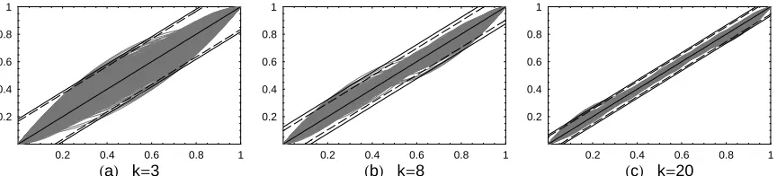
In order to illustrate the bound (22) and how accurately the averaging knot location method (19) solves system (6) with respect to the knots for given Greville sites, we have randomly generated abscissa values xj, j=1, ..., p for three fixed numbers of vertices
p, equal respectively to 6 Hk=3L, 11 Hk =8L and 23 Hk =20L. The number of simula-tions for each value of p is 1000. The corresponding thousand graphs of ⁄ip=1xiNi,nHtL,
tœ @0, 1D, in the quadratic case Hn=3L, with knots defined by (19), are plotted in Fig. 2 (a), (b) and (c).
0.2 0.4 0.6 0.8 1
HaL k=3
0.2 0.4 0.6 0.8 1
0.2 0.4 0.6 0.8 1
HbL k=8
0.2 0.4 0.6 0.8 1
0.2 0.4 0.6 0.8 1
HcL k=20
0.2 0.4 0.6 0.8 1
Fig. 2. Graphs of 1000 simulations of ⁄ip=1xiNi,3HtL, with tk,3 according to (25) and estimates of
e`0.95 and ¶`0.95 for: (a) p=6 Hk=3L, e`0.95=0.17, ¶`0.95 =0.18; (b) p=11 Hk=8L, e`0.95=0.10,
¶`0.95 =0.12; (c) p=23 Hk=20L, e`0.95=0.05, ¶`0.95 =0.07.
In Fig. 2, two corridors are also shown. The first, defined by the dashed lines, is based on the 95 sample percentile of e=∞t-⁄ip=1xiNi,3HtL¥, denoted by e`0.95. The second corridor (the solid lines) is based on the 95 sample percentile ¶`0.95 of the bound in (22), denoted by ¶. As can be seen from Fig. 2, the maximum deviation of ⁄ip=1xiNi,3HtL from the straight line t is reasonable, and rapidly decreases as the number of knots increases. Thus, the higher the number of knots, the more accurately the averaging knot location method (19) solves system (6). Similar conclusions are found to hold for the cubic case (n=4), applying both e`0.95 and ¶`0.95. As seen from Fig. 2, the solid line deviates insig-nificantly from the dashed line, so that the bound in (22) is nearly sharp for n=3.
Remark 3. Note that, as seen from the bounds (16) and (22), the quality of the reconstruc-tion of f`Hdl,2,a`;xL, in stage B, using either CfHtél-Hn-2L,n,a`;xL or CfHtèl-Hn-2L,n,a`;xL, depends on
[image:16.595.82.514.350.448.2]formula (see e.g., Farin 2002) and add a knot at the middle of the interval, where maxjœ81,...,p-1<Hxj+1- xjL is attained. It is worth pointing out that, based on our
experi-ence with GeDS, the reconstruction in stage B is quite satisfactory and such knot inser-tion has not been implemented.
Remark 4. The choice of the knots tèl-Hn-2L,n in (19) can also be given an interpretation,
related to the problem of optimal recovery of a function g, by interpolating it at some fixed points, with an n-th order spline on a set of knots tk,n. The problem is to find the
optimal set of knots, tkopt,n for which the bound on the interpolation error is minimized over all possible choices of tk,n. Such optimal interpolation has been considered by
Michelli, Rivlin and Winograd (1976). An approximate solution to this optimal recovery problem has been proposed by De Boor (2001). In our case, if we apply this scheme to the polygon f`Hdl,2,a`;xL and view its vertices Hxi,a`iL as given data points, then the
approximate solution of this optimal interpolation problem, as proposed by De Boor (2001), is the set of knots tèl-Hn-2L,n in (19).
5. Asymptotic properties of GeDS and related inference.
Pointwise asymptotic properties of the proposed GeD spline estimation method have been explored in Kaishev et al. (2006) where related large sample statistical inference has also been provided. To investigate the pointwise asymptotic behaviour of the GeDS estimation error f`Itèl-Hn-2L,n,q
`
;xM- fHxL its decomposition f`Itèl-Hn-2L,n, q
`
;xM- f HxL
=Af`Itèl-Hn-2L,n,q
`
;xM-E f`Itèl-Hn-2L,n,q
`
;xME+AE f`Iètl-Hn-2L,n,q
`
;xM- fHxLE
has been considered, where the first and the second terms on the right-hand side are correspondingly referred to as the variance and the bias terms. In the asymptotic analy-sis, carried out in Kaishev et al. (2006), as the sample size, Ni, grows to infinity with
i=1, 2, ..., under some mild assumptions with respect to the sequences of design points
8xj<Nj=i1, it has been shown that the knots t
è
li-Hn-2L,n, n¥2, obtained by the GeDS
estima-tion method, have global mesh ratios
Mtè
i
HrL= maxn§j§li+1+n-rHt
ê
i,j+r-têi,jL
ÅÅÅÅÅÅÅÅÅÅÅÅÅÅÅÅÅÅÅÅÅÅÅÅÅÅÅÅÅÅÅÅmin ÅÅÅÅÅÅÅÅÅÅÅÅÅÅÅÅÅÅÅÅÅ
n§j§li+1+n-rHt
ê
i,j+r-têi,jL , r¥n
which form a sequence, bounded in probability by a constant g >0, i.e., Mtè
i
HrL § g,
except on an event whose probability tends to zero as NiØ ¶ (see Lemmas 2 and 3 of
Kaishev et al. 2006).
Based on these results, and on a theorem from approximation theory establishing the stability of the L¶ norm of the L2 projections onto the linear space of splines Stk,n, two
condi-tion for it to be of negligible magnitude compared to the variance term. After its appropri-ate standardization, f`Iètl-Hn-2L,n,q
`
; xM has been shown (see Theorem 3 of Kaishev et al. 2006) to converge to a standard normal distribution, given that a suitable value of aexit in the stopping rule of Stage A has been chosen. This characteristic of GeDS allows for the construction of 100H1- aL% asymptotic confidence intervals
(24) f`Iètl-Hn-2L,n,q
`
;xM≤z1-aê2 "#################################################VarIf
`
Itèl-Hn-2L,n,q
`
;xM … x”÷M, where z1-aê2= F-1H1- aê2L, n¥2 , x”÷=Hx1, ..., xNL,
VarIf`Itèl-Hn-2L,n,q
`
;xM … x”÷M= s2N
n'HxL8XF'Hx”÷L,FHx”÷L\<
-1
NnHxLH1+oPH1LL,
and the matrix FHx”÷L=HNnHx1L, ..., NnHxNLL. In the next section, numerical tests of the
proposed GeD spline estimator are performed and confidence intervals around the final fits are constructed, using the above results.
6. GeDS in action.
The proposed GeDS method has been implemented using Mathematica 5.0 and a stan-dard PC (Pentium IV, 1.4 Ghz, 512 RAM) has been used for all test examples.
In order to obtain a GeDS estimate, most often it is necessary to input only the set of data 8xi, yi<iN=1. The two parameters, aexitœH0, 1L and b œ@0, 1D, defined in steps 10 and 5 of stage A of GeDS (see Appendix A of Kaishev et al. 2006), by means of which the exit from GeDS can be controlled, have default preassigned values, which in general need not be re-set. The parameter aexit is related to the stopping rule, which determines when to exit from stage A, i.e., it determines the number and location of the knots, dl,2, of f`Hdl,2,a`;xL and hence the number and location of the knots of the final higher order LS spline fit f`Itèl-Hn-2L,n,q
`
;xM. The parameter b is related to the cluster weights of the clusters of residuals of same signs, as defined in step 5 of stage A of GeDS (see Appen-dix A of Kaishev et al. 2006). Its choice depends on the wiggliness of the recovered function f and the level of the noise e. In the Normal case, e ~5H0,se2L, the noise level is defined by the variance se2. As will be illustrated, for most of the examples GeDS
gives very good results with the default values aexit=0.9, b =0.5. Our experience shows that choices of aexitœH0, 0.7L may cause exit after the first few steps which, for most functions, does not lead to an adequate resulting fit.
The choice of b depends on the level of the signal-to-noise ratio (SNR), SNR=HvarHfLL0.5êse and on the degree of smoothness of f. As will be seen, in most of
the numerical examples, the appropriate value of b was 0.5, which means that the with-in-cluster mean residual value and the cluster range can be considered equally important components of the weights wj, j=1, ..., l, (see Appendix A of Kaishev et al. 2006).
function then the recommended choice is b œ@0.5, 0.6D, aexitœ@0.99, 0.999D, since otherwise underfitting may result. In the case when SNR is low and f is smooth, one may use b œ@0.4, 0.5D, aexitœ@0.9, 0.99D. It is known that, when the SNR is low and the underlying function is very unsmooth, recovering f is very difficult and different choices of b and aexit may need to be attempted.
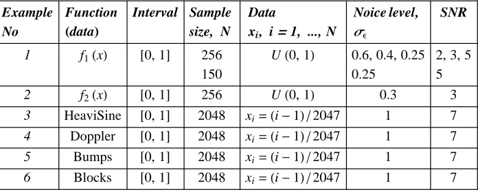
[image:19.595.73.470.248.431.2]In order to facilitate comparison of GeDS with existing smoothing methods, we have simulated data using the functions given in Table 1, which have been widely used in testing other existing smoothing procedures.
Table 1. Summary of test functions.
Function Specification
1 f1HxL=H4x-2L+2‰-16H4x-2L 2
2 f2HxL=sinH8x-4L+2‰-16H4x-2L 2
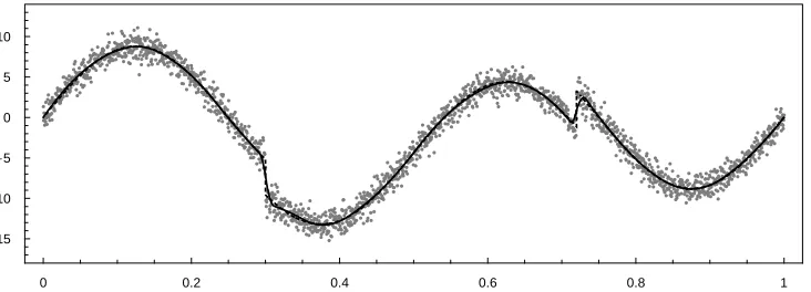
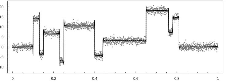
HeaviSine f3HxL=4 sinH4pxL-sgnHx-0.3L-sgnH0.72-xL
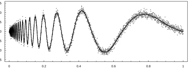
Doppler f4HxL=è!!!!!!!!!!!!!!!!!xH1-xLsinIÅÅÅÅÅÅÅÅÅÅÅÅÅÅÅÅÅÅÅÅ2HpxH+e1+eLLM, e =0.05
Bumps f5HxL=‚
jhjI1+° x-sj
ÅÅÅÅÅÅÅÅÅÅÅÅw
j •M -4
, 8hj<=84, 5, 3, 4, 5, 4.2, 2.1, 4.3, 3.1, 5.1, 4.2< 8sj<=80.1, 0.13, 0.15, 0.23, 0.25, 0.40, 0.44, 0.65, 0.76, 0.78, 0.81<
8wj<=80.005, 0.005, 0.006, 0.01, 0.01, 0.03, 0.01, 0.01, 0.005, 0.008, 0.005< Blocks f6HxL=‚
jhj
1+sgnHx-sjL
ÅÅÅÅÅÅÅÅÅÅÅÅÅÅÅÅÅÅÅÅÅÅÅÅÅÅÅÅÅ2 , 8hj<=84,-5, 3,-4, 5,-4.2, 2.1, 4.3,-3.1, 2.1,-4.2< 8sj<=80.1, 0.13, 0.15, 0.23, 0.25, 0.40, 0.44, 0.65, 0.76, 0.78, 0.81<
The data sets, used to test GeDS were simulated by adding noise, e ~5H0,se2L, to each of the six functions, as given in Table 2.
Table 2. Summary of examples used to test GeDS.
Example No
Function
HdataL
Interval Sample size, N
Data
xi, i=1, ..., N
Noice level,
se
SNR
1 f1HxL @0, 1D 256
150
UH0, 1L 0.6, 0.4, 0.25 0.25
2, 3, 5 5 2 f2HxL @0, 1D 256 UH0, 1L 0.3 3
3 HeaviSine @0, 1D 2048 xi=Hi-1L ê2047 1 7 4 Doppler @0, 1D 2048 xi=Hi-1L ê2047 1 7 5 Bumps @0, 1D 2048 xi=Hi-1L ê2047 1 7 6 Blocks @0, 1D 2048 xi=Hi-1L ê2047 1 7
[image:19.595.77.425.508.648.2]In order to compare the quality of the fits produced by GeDS to those given by other authors, we use the mean square error (MSE), defined with respect to the true function
f, rather than to the data, i.e., MSE=9‚
i=1
N
IfHxiL- f
`
Itèl-Hn-2L,n, q
`
;xiMM
2
= íN.
Note that, in practice, the underlying function is unknown and a set of observations is fitted. For this reason, we give also the L2-error of approximation, defined as è!!!!!!!!!RSS . However, for a fair comparison between the smoothing methods, one would need all model parameter values, such as, the number of knots (regression functions) and degree of the spline fits etc., which often are not reported in full. In order to compare the speed of computation on equal grounds, one would need to implement all of the available methods using the same hardware and software, and test them on entirely identical simulated data sets. Such a comparison is outside the scope of this paper.
Stage A of the GeD spline estimator has been thoroughly illustrated in Kaishev et al. (2006). Here we concentrate on the final GeD spline fit resulting from stage B.
We have run GeDS with 400 simulated data sets for Examples 1 and 2, and 31 data sets for Examples 3-6 as has been done by other authors in testing their methods (see, for example, Luo and Wahba, 1997). This allows us to compute the median of the MSE, obtained using GeDS, and compare it with the MSE medians given by other authors. However, in order to illustrate how GeDS performs, in each example we have used a single data set randomly chosen among the simulated data sets.
We compare most of our results with those of Luo and Wahba (1997) since, along with the median MSE values for their fits, they give also the order and the number of the basis functions. The Bumps and Blocks have been excluded from the comparison, since Luo and Wahba (1997) use versions of these functions which differ from ours, i.e., from those proposed by Donoho and Johnstone (1994). The GeD fits in Examples 1 and 2 are compared with the optimal spline fits, produced following the standard LS non-linear optimization approach and its penalized version, developed by Lindstrom (1999). The latter has been implemented, using the transformation of the knots, proposed by Jupp (1974) and the Mathematica function NMinimize, which attempts to find the global minimum. Due to the drawbacks of the non-linear optimization approach, it has not been feasible to produce optimal spline fits for the spatially inhomogeneous functions, recov-ered in Examples 3-6 from large data sets, using Mathematica, and a standard PC.
Table 3. (Example 1) Summary of fits produced by GeDS.
Fit No
Graph N se n k Internal knots aexit,b L2-error, MSE
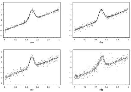
1 Fig. 3,HaL 150 0.25 3 4 80.37, 0.46, 0.54, 0.62< 0.9, 0.5 2.87, 0.001282 2 Fig. 3,HbL 256 0.25 3 4 80.38, 0.46, 0.54, 0.63< 0.9, 0.5 4.01, 0.001359 3 Fig. 3,HcL 256 0.4 3 4 80.38, 0.46, 0.54, 0.60< 0.95, 0.5 6.17, 0.006573 4 Fig. 3,HdL 256 0.6 3 5 80.26, 0.39, 0.51, 0.55, 0.62< 0.95, 0.5 9.03, 0.021918
The L2-errors of all the fits are within the noise level and their visual quality is very good, as can be seen from Fig. 3. The 95% confidence intervals given in Fig. 3 have been calculated using (24) with the corresponding known ('oracle') se.
0 0.2 0.4 0.6 0.8 1
HcL
-3
-2
-1 0 1 2 3
0 0.2 0.4 0.6 0.8 1
HdL
-3
-2
-1 0 1 2 3 0 0.2 0.4 0.6 0.8 1
HaL
-3
-2
-1 0 1 2 3
0 0.2 0.4 0.6 0.8 1
HbL
-3
-2
-1 0 1 2 3
Fig. 3. (Example 1) Graphs of the final quadratic B-spline fits and confidence intervals, produced
by GeDS: (a) N=150, s =0.25; (b) N=256, s =0.25; (c) N=256 , s =0.4 ; (d) N=256, s =0.6; The dotted function is the true function.
Note that the first two fits in Table 3 are obtained with aexit=0.9 and b =0.5. Since the noise levels for fits No 3 and 4 are higher than for fits No 1 and 2, aexit has been increased to 0.95, because, in the case of a smooth function and a high noise level, the relative improvements in RSS from one step to another would be smaller and more steps would be needed to recover the function.
In the case se=0.4, we have compared the quadratic GeD spline fit (No 3, Table 3)
[image:21.595.87.512.284.582.2]method (NOM) and its penalized version (PNOM), due to Lindstrom (1999). The results are summarized in Table 4. As can be seen, the three fits are very close, comparing the L2-errors and the location of the knots. However, the GeD fit recovers the original function significantly better than the fits NOM and PNOM, as indicated by the corre-sponding MSE values. The NOM optimal fit produces an edge at 0.425 and visually deviates stronger from the shape of the underlying function, which is one of the draw-backs noted by Lindstrom (1999). The computation time needed for GeDS is less then a second, and for PNOM and NOM it is respectively 11 and 20 minutes, using the Mathe-matica function NMinimize.
Table 4. (Example 1) The fits produced by GeDS, PNOM and NOM.
Fit No
Method n k Internal knots L2-error, MSE
1 GeDS 3 4 80.38, 0.46, 0.53, 0.60< 6.17, 0.006573 2 PNOM 3 4 80.40, 0.44, 0.52, 0.62< 6.16, 0.007364 3 NOM 3 4 80.42, 0.43, 0.53, 0.60< 6.14, 0.010285
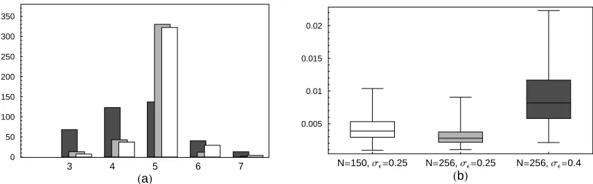
A frequency plot of the number of internal knots and box plots for the three linear GeD spline fits for data sets with N =150, se =0.25, N =256, se =0.25 and
N =256,se=0.4, over the 400 GeDS runs are presented in Fig. 4 (a) and (b).
3 4 5 6 7
HaL
0 50 100 150 200 250 300 350
N=150,se=0.25 N=256,se=0.25 N=256,se=0.4
HbL
0.005 0.01 0.015 0.02
Fig. 4. (a): A frequency plot of the number of knots of the 400 linear GeD spline fits; (b): Box plots
of the MSE values of the 400 linear GeD spline fits;
As can be seen from Fig. 4 (a), the number of knots of the GeD fits for higher noise level (se =0.4) is more dispersed over the range of values 3 to 7, than for the case of
lower noise level Hse=0.25L as is natural to expect. On the other hand, as can be seen
from the box plots in Fig 4 (b), GeDS performs best in the case of larger sample size and lower noise level (N =256,se=0.25 ). The median MSE value of the 400 linear
fits, for se =0.4, with median number of internal knots k=5, is 0.009. This is lower
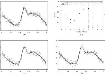
Example 2. The function f2 (see Table 1) appears as a test example in Fan and Gijbels (1995), Luo and Wahba (1997), Denison et al. (1998) and Zhou and Shen (2001). Using the GeDS algorithm we have produced linear, quadratic and cubic fits which are illus-trated in Fig. 5 and whose details are given in Table 5.
0 0.2 0.4 0.6 0.8 1
HcL
-1 0 1 2 3
0 0.2 0.4 0.6 0.8 1
HdL
-1 0 1 2 3 0 0.2 0.4 0.6 0.8 1
HaL
-1 0 1 2 3
0 1 2 3 4 5 6 7 8 9 Number of knots
HbL
0.2 0.4 0.6 0.8 1
RSS
/N a
aexit=0.9
aexit=0.95
Fig. 5. (Example 2) Graphs of the final spline fits and confidence intervals, produced by GeDS: (a)
[image:23.595.96.508.173.464.2]linear; (c) quadratic; (d) cubic; (b) the values of the aratio black dots and the values of RSS/N -grey dots, at each iteration in stage A; The dotted function in (a), (c), (d) is the true function.
Table 5. (Example 2) Summary of fits produced by GeDS.
Fit No
Graph n k Internal knots aexit,b L2-error, MSE
1 Fig. 5,HaL 2 6 80.30, 0.40, 0.50, 0.60, 0.63, 0.83< 0.9, 0.5 4.60, 0.009931 2 Fig. 5,HcL 3 5 80.35, 0.45, 0.55, 0.61, 0.73< 0.9, 0.5 4.63, 0.005961 3 - 4 4 80.40, 0.50, 0.57, 0.69< 0.9, 0.5 4.99, 0.019523 4 - 3 6 80.33, 0.37, 0.45, 0.55, 0.61, 0.73< 0.95, 0.5 4.53, 0.006153 5 Fig. 5,HdL 4 5 80.35, 0.42, 0.50, 0.57, 0.69< 0.95, 0.5 4.51, 0.004258