MORPHOLOGICAL GRANULOMETRY FOR CLASSIFICATION OF EVOLVING
AND ORDERED TEXTURE IMAGES
Mahmuda Khatun
(1), Alison Gray
(1), and Stephen Marshall
(2)(1)Department of Mathematics and Statistics,
University of Strathclyde, Glasgow G1 1XH, UK phone: +44 (0)141 548 4335, fax: +44(0)141 548 3345, email: m.khatun, [email protected]
(2)Department of Electronic and Electrical Engineering,
University of Strathclyde, Glasgow, G1 1XW, UK phone: +44 (0)141 548 2199, fax: +44(0) 141 552 2487, email: [email protected]
ABSTRACT
In this work we investigate the use of morphological gran-ulometric moments as texture descriptors to predict time or class of texture images which evolve over time or follow an intrinsic ordering of textures. A cubic polynomial regression was used to model each of several granulometric moments as a function of time or class. These models are then com-bined and used to predict time or class. The methodology was developed on synthetic images of evolving textures and then successfully applied to classify a sequence of corrosion images to a point on an evolution time scale. Classification performance of the new regression approach is compared to that of linear discriminant analysis, neural networks and sup-port vector machines. We also apply our method to images of black tea leaves, which are ordered according to granule size, and very high classification accuracy was attained compared to existing published results for these images. It was also found that granulometric moments provide much improved classification compared to grey level co-occurrence features for shape-based texture images.
1. INTRODUCTION
Texture classification is a long-standing problem in image processing. It involves a feature extraction step, in which a set of texture features is extracted from the image under study, and a classification step, in which a texture class mem-bership is assigned to it based on the information provided by the extracted texture features through appropriate machine learning algorithms [12]. Here we use morphological granu-lometry and co-occurrence matrix approaches to extract tex-ture featex-tures, and employ a regression-based textex-ture classifi-cation approach to compare the relative usefulness of the two different sets of features for classifying sequences of texture images which either evolve over time or follow an intrinsic ordering. For example, size of texture primitives may in-crease over time or with class label, as in spots of corrosion building up on sheet metal.
Morphological granulometry [13] is extensively used to extract textural information from images. It was first intro-duced to characterise size and shape information for a binary image, considered to be a collection of grains. The concept of granulometry is to sieve the grains through filters of in-creasing size, so that grains with size smaller than the holes will drop out and only grains of larger size will remain. The shape of the holes is determined by the shape of the struc-turing element(SE), which is a geometrical pattern used to extract textural information from a given digital image [6]. In the sieving, the remaining image area successively decreases
and eventually drops to zero. The rate of decrease represents the cumulative proportion of image area dropped, known as thesize distribution[1]. A probability distribution function (pdf) can be derived from this size distribution, since it is a cumulative distribution function (cdf). Its statistical mo-ments, known asgranulometric moments, contain useful tex-tural information to characterise the pdf and the image.
Texture features derived from the grey level co-occurrence matrix (GLCM) [9] are the most widely used texture features for classification. The GLCM represents the probability distribution of occurrence of a pixel pair, at a given separation and at a given orientation, with given grey levels. Various texture features can be derived from the GLCM. GLCM features were successfully used by Chanda and Majumder [3] to segment images of chromosomes. Soh and Tsatsoulis [16] obtained 94.17% classification accuracy for SAR sea ice images using GLCM features in Bayesian classifiers. Clausi [4] computed 8 different GLCM features using different quantisations of SAR sea ice images, and used the features jointly and separately to classify the images.
In this work a regression-based classifier is developed by modelling granulometric moments or GLCM features as a function of texture evolution time or class label. A cubic polynomial regression is fitted for each chosen feature sep-arately, and then a combined cubic polynomial regression is obtained. The combined model is used for back-prediction of evolution time or class label of a new image using its ob-served texture features. Linear discriminant analysis (LDA), neural networks and support vector machines (SVMs) are used with the same sets of features (either granulometric mo-ments or GLCM features) to compare their classification ac-curacy with that of the new regression approach.
We are interested to compare the usefulness of granulo-metric moments and GLCM features in discriminating tex-ture images where textex-tures represent some sort of damage or decay which progresses over time. Knowing the state of damage is vital in many cases, for example, regular mon-itoring of degree of damage of machine parts is of crucial importance in industrial inspection. Classification of images of corroding metal according to their degree of corrosion was studied in [14, 15, 7], and the same set of corrosion images are used here as an example of textures that evolve over time. Another application is the sorting of tea into different grades according to granule size. This is very important task in the tea processing industry, which has traditionally been carried out by sieving with a series of sieves of differ-ently sized mesh. More recdiffer-ently, computer vision and pattern recognition have been investigated for a more automated
proach [2]. We have also applied our methodology to a se-quence of black tea images representing different grades of tea of different granule sizes [2]. This is an example of tex-tures ordered by class.
2. METHODOLOGY
Here we briefly describe the feature extraction methods and different classifiers used.
2.1 Morphological granulometry
Morphological techniques are widely used in digital image processing. The foundation of morphological processing is in set theory. One of the fundamental techniques, i.e. open-ing, provides very useful information about shape and size of image objects or texture primitives. Opening of an image
f by a SE g, denoted by f◦g, is the union of all transla-tions ofgthat are a subset of f. The effect of opening can be explained as sliding SEgbeneath the input image f, elimi-nating any details smaller thangand reducing the height or grey level of larger objects.
Granulometry consists of successive openings of an im-age by a sequence of SEs of increasing size. An im-age f is opened sequentially by a series of scaled SEs {g1,g2, . . . ,gN}, e.g. successively larger disks. At each
stage of opening, the finer details are successively elimi-nated, and the volume of the input image is reduced. Suc-cessive openings create a decreasing sequence of images, i.e.
f◦g1⊃ f◦g2. . .⊃ f◦gN. The image volume remaining
after each opening constitutes a decreasing sequence which eventually reaches zero, i.e. Ω(1)≥Ω(2)≥. . .≥Ω(N), whereΩ(j)is the image volume left after the jth opening. This sequence is called the size distribution [5].
The normalised size distribution represents the cumu-lative proportion of the image volume removed after each opening. It is found by dividing the removed area by the original image volume Ω(0), i.e. Φ(n) =1−Ω(n)/Ω(0). This rises monotonically from 0 to 1 as the size of the SE increases, giving a cumulative distribution function (cdf). Its derivative Φ′(n) =dΦ(n)/dnis a probability density func-tion (pdf). This pdf is referred to as thepattern spectrumin [11]. Since this is a pdf, it possesses statistical moments. These moments can be used for texture classification and analysis. Granulometric moments from the pattern spectrum of the image foreground provide information on object shape, while those from the pattern spectrum of the image back-ground provide information about spatial distribution of the objects. Here we use these moments to predict the time state or class of an image from a sequence of evolving or ordered texture images.
2.2 Grey level co-occurrence matrix (GLCM)
EntryC(i,j)of a GLCM is defined by first specifying a dis-placement d and angleϕ, and counting all pairs of pixels separated by distanced and lying on a line at angleϕ to the reference direction of the image, which have grey levelsiand
jrespectively. The image is often quantised, e.g. to level 8 or 64, before computing the GLCM, to avoid sparsity of the GLCM. The normalised GLCM p(i,j)can be obtained by dividingC(i,j)by the sum of its entries, as
p(i,j) =C(i,j)/
P
∑
k=1
P
∑
l=1
C(k,l),
wherePis the number of grey levels. GCLMs capture prop-erties of a texture but are not directly useful for further analy-sis, such as comparison of two textures. Various texture fea-tures may be computed from the GLCM for more compact texture representation [9, 16, 4], including:
1. Maximum probability : max(i,j)p(i,j)
2. Energy :∑Pi=1∑Pj=1p(i,j)2
3. Entropy :−∑Pi=1∑Pj=1p(i,j)logp(i,j)
4. Contrast: 1
(P−1)2∑Pi=1∑Pj=1(i−j)2p(i,j) 5. Homogeneity:∑Pi=1∑Pj=11p+(|ii,−j)j| 6. Correlation : σ1
iσj∑
P
i=1∑Pj=1(i−µi)(j−µj)p(i,j), where
µi = ∑Pi=1i∑Pj=1p(i,j), µj = ∑Pi=1j∑Pj=1p(i,j), σi = ∑Pi=1(i−µi)2∑Pj=1p(i,j), and σj = ∑Pj=1(j− µj)2∑Pi=1p(i,j).
2.3 Classification methods
Either granulometric moments or GLCM features are mod-elled as a function of time using a cubic polynomial regres-sion approach. LetYi(t),i=1,2, . . . ,p, andt=1,2, . . . ,T
be the average of theith feature for thetthtime or class (av-eraged over the training feature set). The cubic polynomial regression can be written as:
Yi(t) =β
(i)
0 +β
(i)
1 ∗t+β
(i)
2 ∗t 2+β(i)
3 ∗t 3+ξ
i, (1)
where theβ terms are estimated using least squares and the ξiare error terms. We have built one such model for each
fea-ture used and combined them together. For a single feafea-turei
the model will be of the form:
Yi(1)
Yi(2)
.. .
Yi(T)
=
β(i)
0 +β
(i)
1 t1+β
(i)
2 t12+β
(i)
3 t13 β(i)
0 +β
(i)
1 t2+β
(i)
2 t22+β
(i)
3 t23 ..
. β(i)
0 +β
(i)
1 tT+β2(i)tT2+β
(i)
3 tT3
+ ε1 ε2 .. . εT .
Forp such features, the combined fitted model relating each feature to time or class is:
ˆ
Y1(t) ˆ
Y2(t) .. . ˆ
Yp(t)
= ˆ β(1)
0 +βˆ
(1)
1 t+βˆ
(1)
2 t2+βˆ
(1)
3 t3 ˆ
β(2)
0 +βˆ
(2)
1 t+βˆ
(2)
2 t2+βˆ
(2)
3 t3 ..
. ˆ
β(p)
0 +βˆ
(p)
1 t+βˆ
(p)
2 t 2+βˆ(p)
3 t 3 , (2)
or equally ˆ
Y1(t) ˆ
Y2(t) .. . ˆ
Yp(t)
= ˆ β(1)
0 ˆ β(2)
0 .. . ˆ β(p)
0 + ˆ β(1)
1 βˆ
(1)
2 βˆ
(1)
3 ˆ
β(2)
1 βˆ
(2)
2 βˆ
(2)
3 ..
. ˆ β(p)
1 βˆ
(p)
2 βˆ
(p)
3 tt2
Using matrix-vector notation this can be written as:
[
ˆ
Y−β0ˆ ]=[ β1ˆ β2ˆ β3ˆ ]
tt2
t3
(3)
or [ Yˆ −β0ˆ ]=BTˆ .
Pre-multiplying by(Yˆ −β0ˆ )T, we get
(Yˆ−β0ˆ )T(1×p)(Yˆ−β0ˆ )(p×1)= (Yˆ−β0ˆ )T(1×p)Bˆ(p×3)T(3×1).
(4)
Equation (4) can be written asat3+bt2+ct+d=0. A positive real root of this equation is used as the predicted time or class. Where there is more than one positive real root we choose the smallest one (as was appropriate in all our training examples). If none of the roots are positive and real the method fails to predict time, and we choose the first time point or class as the prediction.
We compare performance of this regression approach with three other classifiers used to classify objects into mutu-ally exclusive and exhaustive classes based on a set of mea-surable object features. Linear discriminant analysis (LDA) [8] is a statistical technique which assigns a new feature vec-tor x to the class which has highest posterior probability, assuming the class conditional distributions are multivariate normal with common covariance matrix. The proportions of the data in each time or class are used as prior probabili-ties. A feed-forward single hidden layer neural network [10] is also used, with 5 units in the hidden layer chosen for opti-mal performance (in training we tried between 2 and 7 units). Since the performance of SVMs is greatly affected by the choice of kernel function and its associated parameter val-ues, different kernels with different combinations of parame-ter values and the cost constraint were experimented with to tune the SVM for better performance. One-to-one classifica-tion is used here as a means of multi-class classificaclassifica-tion. A detailed account of SVMs can be found in [10].
The prediction abilities of the classifiers are assessed us-ing proportion of misclassifications and mean absolute error (MAE), defined as:
MAE =1
n
n
∑
i=1
|tipred−tacti |, (5)
wherenis the number of images for which time or class is to be predicted, andtipredandtacti are respectively the (rounded) predicted and actual state of time or class of imagei.
3. APPLICATION TO REAL IMAGES
3.1 Corrosion images
We applied our methodology to a set of real corrosion images generated in [15]. These are images of a steel plate corroded over a period of 10 consecutive days and photographed daily. The original colour images are of size 14002and were con-verted to grey scale. To obtain training and test sets, 10 non-overlapping images of size 2562were extracted from each of the grey scale images at timest=1, . . . ,10. So there are a total of 100 sample images, 10 for each time point.
As the images were converted from colour images show-ing substantial intensity variations, image pre-processshow-ing
was needed. Spots within the images are darker than the background, so the bottom-hat transform is appropriate for pre-processing. Subtracting the original image from the opened image produces the bottom-hat transform
f•ˆg= (f•g)−f.
We use a disk SE of increasing size asg, since the corrosion spots increase in size over time. A wide range of radius val-ues were tested and the most appropriate ones (6, 7, 8,. . ., 15) were chosen for times 1 through 10 to preserve best the sizes and shapes of the textures. Figure 1 shows some of the extracted grey scale corrosion images and their bottom-hat transformed images.
(a)t=1 (b) Bottom-hat image of (a)
(c)t=5
(d) Bottom-hat image of (c)
[image:3.595.315.536.230.412.2](e)t=10 (f) Bottom-hat image of (e)
Figure 1: Grey scale corrosion sub-images of size 2562and their bottom-hat transformed images at timest=1,t=5 and
t=10.
The first four granulometric moments computed from the bottom-hat transformed images using square and disk SEs are shown in Table 1. Average granulometric mean and stan-dard deviation (sd) using both SEs clearly increase over time, while skewness decreases. Kurtosis does not vary much over time, however in the results below we use all 4 moments from both SEs.
Since there are 10 sub-images at each time point t =
1,2, . . .10, the moments data form a 100×8 matrix. A ran-domly selected sub-set of 70% of the moments are used to fit the cubic polynomial regression in Equations 1–3 and the rest are used to predict as in Equation 4. The procedure was repeated 10 times and average results were obtained. The same approach was used for LDA, the neural network and the SVM as well.
3.2 Tea images
Table 1: First four granulometric moments for the bottom-hat transformed corrosion images using square and disk SEs.
Time Moments using square SE
mean sd skewness kurtosis
1 6.6565 4.5828 0.0032 -2.9977
2 7.5256 5.4877 0.0022 -2.9989
3 8.8921 6.2471 0.0014 -2.9993
4 10.1779 7.2285 0.0009 -2.9996
5 11.2492 7.9117 0.0007 -2.9997
6 12.4619 8.9238 0.0005 -2.9998
7 13.7676 10.1043 0.0004 -2.9999
8 14.8493 11.2805 0.0003 -2.9999
9 17.6761 12.6737 0.0002 -3.0000
10 17.8071 13.8678 0.0002 -3.0000
Moments using disk SE
mean sd skewness kurtosis
1 3.2607 2.6405 0.0227 -2.9817
2 3.7773 3.1449 0.0141 -2.9908
3 4.5955 3.5949 0.0085 -2.9945
4 5.3489 4.1534 0.0054 -2.9969
5 5.9891 4.5508 0.0041 -2.9978
6 6.6898 5.0891 0.0029 -2.9986
7 7.4305 5.6975 0.0020 -2.9991
8 7.9708 6.1374 0.0016 -2.9993
9 9.5363 6.7399 0.0010 -2.9995
10 9.5141 7.4247 0.0008 -2.9997
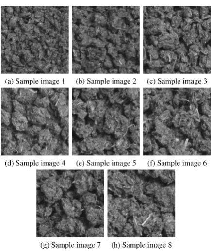
[image:4.595.59.277.462.721.2]2562size images from each of the original images and con-verted them to grey scale. Fifty non-overlapping sub-images were extracted from one image from each class, giving 400 sample images. One sub-image from each class is shown in Figure 2, to show the increasing size of the tea granules over classes.
(a) Sample image 1 (b) Sample image 2 (c) Sample image 3
(d) Sample image 4 (e) Sample image 5 (f) Sample image 6
(g) Sample image 7 (h) Sample image 8
Figure 2: Sample grey scale tea images of size 2562, one from each of the eight classes.
There is substantial variation of intensity within the im-ages. To improve this, a top-hat transformation was applied as pre-processing. Since granule size increases over classes, a disk SE of increasing size is used in the top-hat transform (with radii 13, 15, 17,. . ., 27). We applied granulometry on the transformed images using square and disk SEs separately and computed the first four PS moments from the pattern spectrum from each SE. Average PS moments are calculated using all sub-images from each class to give an 8×8 data ma-trix. Again we implemented the regression approach, LDA, neural network and SVM classifiers and compared their per-formance.
4. ANALYSIS AND FINDINGS
For all classifiers 70% of the moments data, randomly se-lected, was used for training and the rest for testing. This was repeated 10 times and results were averaged.
[image:4.595.325.528.463.596.2]For the corrosion images, Table 2 shows the performance of all classifiers using the granulometric moments. No im-age was misclassified by more than one time point, so the MAE and misclassification rate are equal. For the regres-sion approach, 29 images are misclassified out of 300, giv-ing 90.27% correct classification. The SVM usgiv-ing the radial basis kernel is the best, with an average correct classifica-tion rate of 99.33% (using cost=100 and kernel parameter γ=0.9). Similar results can be obtained for many parame-ter settings. LDA is the second best classifier with 93.67% correct classification. The neural network with optimum pa-rameter setting produces a higher misclassification rate. The regression approach is better than the neural network.
Table 2: Time-wise MAE or misclassification rate using all classifiers with 8 granulometric moments, for the corrosion images.
Time Error rate
Regression SVM LDA NNET
1 0.0000 0.0000 0.0000 0.0000
2 0.0000 0.0000 0.1333 0.0333
3 0.0000 0.0000 0.0000 0.0000
4 0.0333 0.0000 0.0000 0.1333
5 0.1000 0.0000 0.1333 0.2000
6 0.0000 0.0000 0.1000 0.3333
7 0.0067 0.0000 0.0667 0.2667
8 0.0333 0.0000 0.1000 0.2667
9 0.4667 0.0000 0.0667 0.3333
10 0.3333 0.0667 0.0333 0.1000
Overall 0.0973 0.0067 0.0633 0.1667
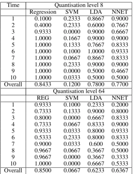
Table 3: Error rates for all classifiers using 6 GLCM features at quantisation levels 8 and 64, for the corrosion images.
Time Quantisation level 8
Regression SVM LDA NNET 1 0.1000 0.2333 0.8667 0.9000 2 0.4000 0.2333 0.6000 0.7667 3 0.9333 0.0000 0.9000 0.6667 4 1.0000 0.1667 0.9000 0.9000 5 1.0000 0.1333 0.7667 0.8333 6 1.0000 0.1000 1.0000 0.9333 7 1.0000 0.0667 0.8667 0.8333 8 1.0000 0.2333 0.9000 0.9000 9 1.0000 0.0000 0.5000 0.4667 10 1.0000 0.0333 0.5000 0.5000 Overall 0.8433 0.1200 0.7800 0.7700
Quantisation level 64
REG SVM LDA NNET
1 0.9333 0.1000 0.2333 0.2000 2 0.7333 0.1333 0.9000 0.8000 3 0.8000 0.0000 0.6667 0.8333 4 0.7333 0.0667 0.8333 0.9000 5 0.9333 0.0333 0.8000 0.9333 6 0.5333 0.2333 0.8000 0.8333 7 0.9000 0.0333 0.600 0.5000 8 0.9667 0.0667 0.3667 0.5000 9 0.9667 0.0000 0.3667 0.3333 10 1.0000 0.0000 0.6667 0.5333 Overall 0.8500 0.0667 0.6233 0.6367
The new regression-based method for classifying images of corrosion to a point in time substantially improves on the results from the approach in [14, 15, 7], where the lowest misclassification rate for the corrosion images was as high as 48%.
For the tea images, the regression classifier produced 89.50% correct classification using granulometric moments, however 100% correct classification can be obtained using all other classifiers if appropriate parameter values are cho-sen. All the classifiers outperform previous results for these images as reported in [2]. Our highest misclassification rate of 10.50% is for the regression approach, using top-hat trans-formed images, whereas the lowest misclassification rate in [2] was 20%.
5. SUMMARY AND CONCLUSIONS
In this paper, a regression-based classification approach was applied to two sets of real images and improved results are obtained compared to the existing published work on these images. Increasing the radius of the disk SE in the bottom-or top-hat transfbottom-orm of the images is of crucial impbottom-ortance, as granulometric features computed from the hat transformed images obtained using the same size disk SE over all time points or classes produced very high classification error for all classifiers. Our results are not exactly comparable to [14] and [2], as we have extracted our own sub-images for al-gorithm development and testing. Nonetheless we conclude that extracting shape-based information from the images di-rectly by use of morphological techniques provides very use-ful features compared to GLCM features for texture
classifi-cation in any of a range of classifiers.
REFERENCES
[1] Batman, S. and Dougherty, E.R. (1997). Size distri-butions for multivariate morphological granulometries: texture classification and statistical properties. Optical Engineering, 36(5), 1518-1529.
[2] Borah, S., Hines, E.L. and Bhuyan, M. (2007). Wavelet transform based image texture analysis for size estima-tion applied to the sorting of tea granules. Journal of Food Engineering, 79, 629-639.
[3] Chanda, B. and Majumder, D. (1988). A note on the use of the gray level co-occurrence matrix in threshold selec-tion. Journal of Signal Processing, 15(2), 149-167. [4] Clausi, D.A. (2002). An analysis of co-occurrence
tex-ture statistics as a function of grey level quantization. Canadian Journal of Remote Sensing, 28(1), 45-62. [5] Dougherty, E.R. and Lotufo, R.A. (2003). Hands-on
Morphological Image Processing. SPIE Press, Washing-ton, USA.
[6] Gonzalez, R.C. and Woods, R.E. (2008). Digital Image Processing, Third Edition. Prentice Hall, New Jersey. [7] Gray, A.J., Marshall, S. and McKenzie, J. (2006).
Mod-eling of evolving textures using granulometries. In Mar-shall, S. and Sicuranza, G.L. (eds.), Advances in Non-linear Signal and Image Processing, EURASIP Series on Signal Processing and Communications, Hindawi Pub-lishing Corporation, New York.
[8] Hand, D.J. (1981). Discrimination and Classification. John Wiley and Sons Ltd, Chichester, UK.
[9] Haralick, R.M., Shanmugan, K. and Dinstein, I. (1973). Textural features for image classification. IEEE Transac-tions on Systems, Man and Cybernetics, 3(6), 610-621. [10] Izenman, A.J. (2008). Modern Multivariate Statistical
Techniques: Regression, Classification, and Manifold Learning. Springer, USA.
[11] Maragos, P. (1989). Pattern spectrum and multiscale shape representation. IEEE Transactions on Pattern Analysis and Machine Intelligence, 11(7), 701-716. [12] Masotti, M. and Campanini, P. (2008). Texture
classifi-cation using invariant ranklet features. Pattern Recogni-tion Letters, 29(14), 1980-1986.
[13] Matheron, G. (1975). Random Sets and Integral Geom-etry. John Wiley and Sons Ltd, New York.
[14] McKenzie, J., Marshall, S., Gray, A.J. and Dougherty, E.R. (2003). Morphological texture analysis using the texture evolution function. International Journal of Pat-tern Recognition and Artificial Intelligence, special issue on Quantitative Image Morphology, 17(2), 167-185. [15] McKenzie, J. (2004). Classification of dynamically
evolving textures using evolution functions. Ph.D. The-sis, Department of Electronic and Electrical Engineer-ing, University of Strathclyde, Glasgow.