Published online in Wiley Online Library (wileyonlinelibrary.com) DOI: 10.1002/qre.1212
Application of Six Sigma Methodology
to Reduce Defects of a Grinding Process
E. V. Gijo
a
, Johny Scaria
b
and Jiju Antony
c
∗
†
Six Sigma is a data-driven leadership approach using specific tools and methodologies that lead to fact-based decision making. This paper deals with the application of the Six Sigma methodology in reducing defects in a fine grinding process of an automotive company in India. The DMAIC (Define–Measure–Analyse–Improve–Control) approach has been followed here to solve the underlying problem of reducing process variation and improving the process yield. This paper explores how a manufacturing process can use a systematic methodology to move towards world-class quality level. The application of the Six Sigma methodology resulted in reduction of defects in the fine grinding process from 16.6 to 1.19%. The DMAIC methodology has had a significant financial impact on the profitability of the company in terms of reduction in scrap cost, man-hour saving on rework and increased output. A saving of approximately US$2.4 million per annum was reported from this project. Copyright©2011 John Wiley & Sons, Ltd.
Keywords: Six Sigma; Kappa statistic; process capability evaluation; chi-square test; ANOVA; Taguchi methods
1.
Introduction
S
ix Sigma is a well-structured methodology that focuses on reducing variation, measuring defects and improving the quality of products, processes and services. Six Sigma methodology was originally developed by Motorola in 1980s and it targeted a difficult goal of 3.4 parts per million defects1. Six Sigma has been on an incredible run over 25 years, producing significant savings to the bottom line of many large and small organizations2. Leading organizations with a track record in quality have adopted Six Sigma and claimed that it has transformed their organization3. Six Sigma was initially introduced in manufacturing processes; today, however, marketing, purchasing, billing, invoicing, insurance, human resource and customer call answering functions are also implementing the Six Sigma methodology with the aim of continuously reducing defects throughout the organization’s processes4.According to Harry and Schroeder5, Six Sigma is a powerful breakthrough business improvement strategy that enables companies to use simple and powerful statistical methods for achieving and sustaining operational excellence. It is a business strategy that allows companies to drastically improve their performance by designing and monitoring everyday business activities in ways that minimize waste and resources while increasing customer satisfaction6. The Six Sigma approach starts with a business strategy and ends with top-down implementation, having a significant impact on profit, if successfully deployed3. Numerous books and articles provide the basic concepts and benefits of the Six Sigma methodology. These publications cover topics, such as What is Six Sigma3? Why do we need Six Sigma7? Six Sigma deployment8; critical success factors of the Six Sigma implementation4; Hurdles in the Six Sigma implementation9; the Six Sigma project selection10 and organizational infrastructure required for implementing Six Sigma11. Numerous articles are available in different aspects of Six Sigma over the past 10 years12--17. The Six Sigma approach has been widely used to improve performances and reduce costs for several industrial fields18--22.
This paper presents the step-by-step application of the Six Sigma DMAIC (Define–Measure–Analyse–Improve–control) approach to eliminate the defects in a fine grinding process of an automotive company. This has helped to reduce defects in the process and thereby improve productivity and on time delivery to customer. During the measure and analyse phases of the project, data were collected from the processes to understand the baseline performance and for validation of causes. These data were studied through various graphical and statistical analyses. Chi-square test, ANOVA23, Design of Experiments (DOE)24, Control Charts25, Taguchi methods26, etc. were used to make meaningful and scientifically proven conclusions about the process and the related causes.
aSQC & OR Unit, Indian Statistical Institute, 8th Mile, Mysore Road, Bangalore 560 059, India bDepartment of Statistics, Nirmala College, Muvattupuzha 686 661, India
cDepartment of DMEM, University of Strathclyde, Glasgow, Scotland G1 1XJ, U.K.
The structure of this article is as follows. The research methodology adopted for this study is explained in Section 2. Section 3 explains an introduction to the case study, Section 3.1 indicates the define phase, Section 3.2 details the measure phase with baseline performance. The Analyse phase is explained in Section 3.3 with details of potential causes and its validation followed by the Improvement phase in Section 3.4 with details of solutions implemented. Section 3.5 explains the controls introduced to ensure sustainability of the results. Section 4 provides information about the lessons learned followed by Section 5, the managerial implications of the initiative. Section 6 presents the concluding remarks and discusses the benefits and limitations of the study.
2.
Research methodology
This section explains the methodology adopted for this case study. Scientific investigation on innovating a system or improvement to the existing one needs to begin with some structure and plan. This structure and plan of investigation were conceived so as to obtain answers to research questions in the research design27. The researcher worked with the company to provide support for the project in the Six Sigma techniques, whilst recording data about the exercise from which to develop a case study. A literature review was undertaken with an objective of identifying the past history of various improvement initiatives carried out to address process-related problems.
The methodology is divided into four major sections namely problem definition, literature survey, case study design and data analysis. Based on the available data on the process, the team studied the baseline status of the process and drafted a project charter, which explains the details of the problem. A detailed literature review was undertaken in Six Sigma with an objective of identifying the type of improvements carried out by different people in various organizations to address process-related problems.
A case study entails the detailed and intensive analysis of a single case—a single organization, a single location or a single event28. Yin29 describes a case study as an empirical inquiry that investigates a contemporary phenomenon within its real-life context. According to Lee30, the unit of analysis in a case study is the phenomenon under study and deciding this unit appropriately is central to a research study. In this paper, a case study is designed to study the underlying process problem so that solutions can be implemented for process improvement. The collected data were analysed using descriptive and inferential statistics. Measurement system analysis, chi-square test, ANOVA, DOE with Taguchi methods, etc. were used for analysing the data and inferences were made. Graphical analyses, such as histogram and control chart, were also utilized for summarizing the data and making meaningful conclusions. Minitab statistical software was used to analyse the data collected at different stages in the case study.
3.
Case study
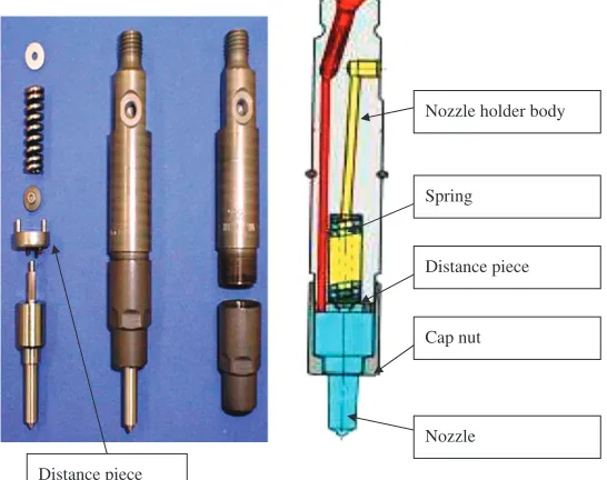
This case study deals with the reduction of defects in the fine grinding process in an automobile part manufacturing company in India. The company with manpower of approximately 2550 people is manufacturing common rail direct injection (CRDI) system pumps for vehicles. These pumps were used in cars, trucks and buses throughout the world. An injector primarily consists of nozzle and nozzle holder body. A schematic view of fuel injector is given in Figure 1. The components used in fuel injector and
Nozzle holder body
Spring
Distance piece
Nozzle Cap nut
[image:2.594.161.434.498.714.2]Distance piece
their functions are as follows. Distance piece aligns the high-pressure fuel lines of nozzle holder body and nozzle. Its both sides are fine ground precisely to ensure sealing of the high-pressure fuel coming from holder body to nozzle. Cap nut retains the nozzle and distance piece with the holder body with sufficient torque to ensure sealing. Spring and pressure bolt ensures the functioning of injector with set opening pressure and timely delivery of fuel.
The current project was undertaken in the distance piece fine grinding process, which is done by fine grinding machine. Different types of distance pieces were fine ground in this machine. This is a sophisticated and very expensive CNC fine grinding machine. It finishes both faces of distance pieces in batches precisely with sub-micron flatness values.
After fine grinding, distance pieces were inspected visually to find various defects. Since the production of distance pieces were in thousands per shift, it was not practically possible to do 100% inspection of these components by objective methods. Hence visual inspection was carried out for all the components with reference to master pieces and visual limit samples. Since the rejection level of distance pieces after fine grinding process was very high and the function of the component in the product was highly critical, it was essential to do 100% inspection. Under these circumstances, the project was of highest priority to the management as it was clear that an effective solution to this problem would have a significant impact in reducing rework/ rejection and improving productivity. Also, it was clear to the team members and champion of the project that the elimination of this problem will help the organization to cater to the increasing demand of market. In the past, many attempts were made to solve this problem by using different methodologies, which were unsuccessful. The Six Sigma problem solving methodology (DMAIC) was recommended when the cause of the problem is unclear3. Hence, it was decided to address this problem through the Six Sigma DMAIC methodology.
3.1. Define phase
This phase of the DMAIC methodology aims to define the scope and goals of the improvement project in terms of customer requirements and to develop a process that delivers these requirements. The first step towards solving any problem in the Six Sigma methodology is by formulating a team of people associated with the process. The team selected for this project includes the Senior Manager—Manufacturing as the Black Belt (BB). The other members of the team were Planning Manager, Maintenance Manager, Quality Control Senior Engineer and one Machine Operator. BB acts as the team leader, and was responsible for the overall success of the project. In this particular project, BB himself was the process owner. The primary responsibility of team members was to support BB in executing the project-related actions. The Head of manufacturing department was identified as the Champion and the Head of Business Excellence department as master black belt (MBB) for this project. The team along with the Champion and MBB developed a project charter (Appendix 1) with all necessary details of the project. This has helped the team members to clearly understand the project objective, project duration, resources available, roles and responsibilities of team members, project scope and boundaries, expected results from the project, etc. This creates a common vision and sense of ownership for the project, so that the entire team is focused on the objectives of the project.
The team had several meetings with the Champion and MBB to discuss various aspects of the problem, including the internal and customer-related issues arising because of this problem. The team decided to consider the rejection percentage of distance pieces after fine grinding process as the Critical to Quality (CTQ) characteristic for this project. The goal statement was defined as the reduction in rejection of distance pieces by 50% from the existing level, which should result in large cost saving for the company in terms of reduction in rework and scrap cost.
Since there was a cross-functional team for executing this project, the team felt that it was necessary to perform a SIPOC (Supplier–Input–Process–Output–Customer) analysis to have a better understanding of the process. This is a method similar to process mapping for defining and understanding process steps, process inputs and process outputs3. The team with the involvement of people working with the process prepared a SIPOC mapping along with a basic flowchart of the process. This SIPOC has given a clear understanding of the process steps needed to create the output of the process. Through this exercise, the team got the clarity of the project in terms of the scope of the project, inputs, outputs, suppliers and customers of the process. The team focused on the fine grinding process for improvement that is defined as the scope of the project. The process mapping along with SIPOC is presented in Appendix 2.
3.2. Measure phase
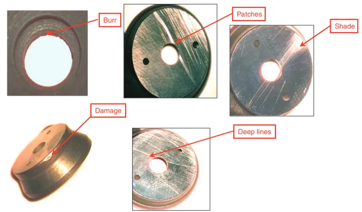
The objective of the measure phase is to understand and establish the baseline performance of the process in terms of process capability or sigma rating. The CTQ considered in this case was the rejection percentage of distance pieces after the fine grinding process. These rejections were mainly due to the occurrence of different types of defects, such as burr, shades, deep lines, patches and damage, on the component after machining. The schematic representation of these defects is presented in Figure 2. These defects create an uneven surface in the component that could lead to fuel leakages in pumps. After machining, the components were visually inspected for these defects. Master samples were provided for identifying each of these defects and inspectors did the inspection. Since there was no instrument involved in the inspection process and only visual inspection was performed, before going ahead with further data collection, the team decided to carry out Attribute Gage Repeatability and Reproducibility (Gage R & R) study to validate the measurement system. In such studies, intra-inspector agreement measures repeatability (within inspector), inter inspector agreement measures the combination of repeatability and reproducibility (between inspectors)31. The non-chance agreement between the two inspectors, denoted byKappa, defines as
Deep lines Patches Burr
Damage
Shade
[image:4.594.109.479.64.281.2]Figure 2. Schematic representation of defects
Table I. Data collection plan
Characteristic Data type How measured Sampling notes Related conditions
Rejection percentage of distance pieces after the fine grinding process
Attribute Visual checking by comparing with visual limit samples
100% of units in all the three shifts for two months
Shift wise and defect type wise
For conducting the study, 100 components were selected and they were classified as good or bad independently by two inspectors. From the resulting data, the Kappavalue was calculated and was found to be 0.814 with a standard error of 0.0839. Since theKappavalue was more than 0.6, the measurement system was acceptable31.
After the measurement system study, a data collection plan was prepared with details of types of data, stratification factors, sampling frequency, method of measurement, etc. for the data to be collected during the measure phase of this study. The data collection plan thus prepared is presented in Table I. The data were collected as per the plan to understand the baseline status of the process. During the defined period of data collection, 368 219 components were inspected and 61 198 components were rejected due to various defects. Each one of the rejected components was having one or more defects. The detailed data on the type of defects were collected and the same was graphically presented as a pareto diagram (Figure 3). The collected data shows that the rejection in the process was 166 200 PPM. The correspondingsigma ratingof the process can be approximated to 2.47.
For any improvement initiative in this organization, the general goal set by the management was to reduce the rejection by 50% from the existing level. Based on this policy, the target set for the study was to reduce the rejections at the fine grinding process to 83 100 PPM from the existing level of 166 200 PPM.
3.3. Analyse phase
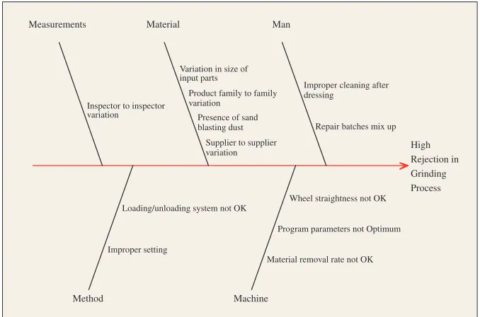
After mapping the process, the team proceeded to analyse the potential causes of defects. A cause and effect diagram was prepared after conducting a brain storming session with all the concerned people from the process along with the project team, Champion and MBB. The output of the cause and effect diagram depends on a large extent on the quality and creativity of the brain storming session32. Figure 4 illustrates the cause and effect analysis prepared during the brain storming session.
Count Perc
e
n
t
Defect Count
0.2
Cum % 42.3 75.5 99.8 100.0
76539 60267 43995 318
Percent 42.3 33.3 24.3
Others Patches
Deep lines Shades
200000
150000
100000
50000
0
100
80
60
40
20
[image:5.594.128.466.67.291.2]0
Figure 3. Pareto diagram for visual defects
High Rejection in Grinding Process Measurements
Method
Material
Machine Man
Repair batches mix up Improper cleaning after dressing
Wheel straightness not OK
Program parameters not Optimum
Material removal rate not OK Supplier to supplier
variation Presence of sand blasting dust Product family to family variation
Variation in size of input parts
Loading/unloading system not OK
Improper setting Inspector to inspector variation
Figure 4. Cause and effect diagram for rejection in grinding process
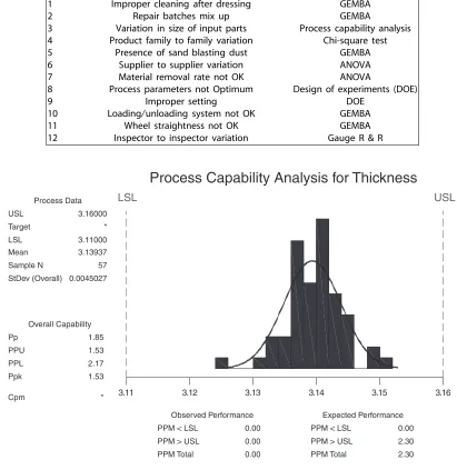
[image:5.594.127.466.339.563.2]Table II. Cause validation plan
Sl. no Cause Plan for validation
1 Improper cleaning after dressing GEMBA
2 Repair batches mix up GEMBA
3 Variation in size of input parts Process capability analysis
4 Product family to family variation Chi-square test
5 Presence of sand blasting dust GEMBA
6 Supplier to supplier variation ANOVA
7 Material removal rate not OK ANOVA
8 Process parameters not Optimum Design of experiments (DOE)
9 Improper setting DOE
10 Loading/unloading system not OK GEMBA
11 Wheel straightness not OK GEMBA
12 Inspector to inspector variation Gauge R & R
3.11 3.12 3.13 3.14 3.15 3.16
LSL USL
Process Capability Analysis for Thickness
USL Target LSL Mean Sample N StDev (Overall)
Pp PPU PPL Ppk
Cpm
PPM < LSL PPM > USL PPM Total
PPM < LSL PPM > USL PPM Total 3.16000
* 3.11000 3.13937 57 0.0045027
1.85 1.53 2.17 1.53
*
0.00 0.00 0.00
0.00 2.30 2.30 Process Data
Overall Capability
Expected Performance Observed Performance
Figure 5. Process capability analysis
Since different families of products were produced, data were collected for material removal rate (MRR) as well as defects with respect to various families of components to test their significance. Data on MRR were collected on three types of components to study the effect of type of component on MRR. Based on the quantity of material removed from the component during machining, the MRR value was calculated by an inbuilt software program in the machine. These MRR data were recorded in millimeter/minute. ANOVA was performed on this data andp-valuewas found to be 0.085, not showing significance at 5% level23. To test whether product family-to-family variation affects the defects, a chi-square test was carried out between defect type and family of components23. For each of the defect types, viz., patches, shades and deep lines, separate chi-square test was done with three different families of components. The details of chi-square test are given in Table III. From Table III, it was clear that except for shades, family-to-family variation does not affect visual defects. The machining program and machine parameters for each family and type were different. The team thought, it was better to have a uniform machining program and parameters for all the family components so that the process can be better managed. Hence for validating the process parameters and identifying the optimum operating conditions, the team decided to conduct a DOE during the improve phase. DOE is a technique for understanding variability, in which factors are systematically and simultaneously manipulated while the variability in outputs (responses) is studied to determine which factors have the biggest impact24.
[image:6.594.88.499.106.529.2]Table III. Test statistic values for Chi-square test
Defect type Chi-square statistic Degrees of freedom p-value
Patches 2.509 2 0.285
Deep lines 2.398 2 0.301
Shades 452.256 2 0.000
Table IV. Gemba observations
Sl. no. Cause Observation/conclusion
1 Improper cleaning after dressing It was observed that cleaning done after dressing. Not a root cause.
2 Repair batches mix up Repair batches were found mixed with other batches during the random visit to the process. Root cause.
3 Presence of sand blasting dust Traces of shot blasting dust found in the input batch during inspection. Root cause.
4 Loading/unloading system not OK Loading table wear out observed at the edges. Root cause.
[image:7.594.93.500.308.474.2]5 Wheel straightness not OK Wheel straightness found OK. Checking frequency followed as per procedure. Not a root cause.
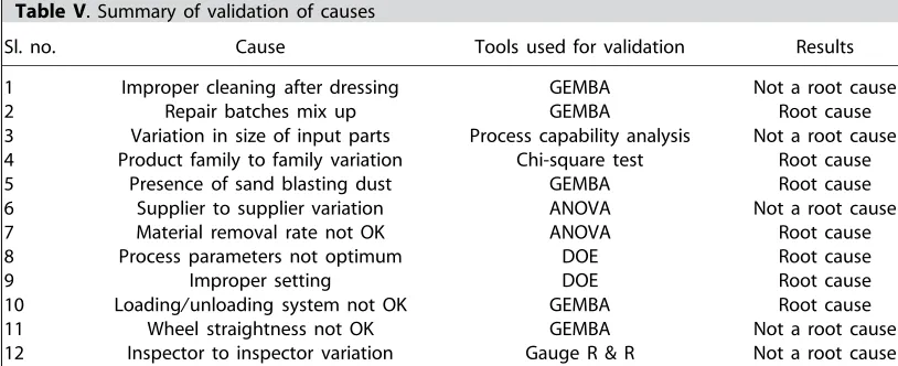
Table V. Summary of validation of causes
Sl. no. Cause Tools used for validation Results
1 Improper cleaning after dressing GEMBA Not a root cause
2 Repair batches mix up GEMBA Root cause
3 Variation in size of input parts Process capability analysis Not a root cause
4 Product family to family variation Chi-square test Root cause
5 Presence of sand blasting dust GEMBA Root cause
6 Supplier to supplier variation ANOVA Not a root cause
7 Material removal rate not OK ANOVA Root cause
8 Process parameters not optimum DOE Root cause
9 Improper setting DOE Root cause
10 Loading/unloading system not OK GEMBA Root cause
11 Wheel straightness not OK GEMBA Not a root cause
12 Inspector to inspector variation Gauge R & R Not a root cause
3.4. Improve phase
This phase of the Six Sigma project is aimed at identifying solutions for all the root causes identified during the Analyse phase, implementing them after studying the risk involved in implementation and observing the results.
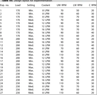
At this stage, as decided earlier, a DOE was planned for optimizing the process/machine parameters. The team along with champion, MBB, the production supervisor and operators of the process conducted a series of brain storming sessions to identify the important parameters for experimentation. The parameters selected through these discussions wereload applied,initial load setting,coolant flow rate,upper wheel rpm,lower wheel rpmand cage rpm. Since the relationship between these parameters and MRR was not known, it was decided to experiment all these parameters at three levels26. The existing operating level was selected as one level for experimentation. The team based on various operational feasibilities selected the other two levels. The parameters and levels selected for experimentation are presented in Table VI. Also, the team felt there is a possibility of interaction between load appliedwithupper wheel rpm,load appliedwithlower wheel rpmandload appliedwithcage rpm. Hence it was decided to estimate the effect of these three interactions also. Six parameters at three levels and three interactions with replications require a huge number of components for conducting a full factorial experiment, which would be a costly and time-consuming exercise24. It was possible to estimate the effect of these selected parameters and interactions using the 27 experiments with the help of Orthogonal Array (OA). Hence for conducting an experiment with six parameters and three interactions,L27(313) orthogonal array was selected34. As the name suggests, the columns of this array are mutually orthogonal. Also, experiments using orthogonal arrays play a crucial role in achieving additivity of the model effects34. The design layout prepared as perL27(313) orthogonal array is given in Table VII. The response of the experiment was decided as material removal rate (MRR).
Table VI. Process parameters and their levels
Sl. no. Factor Levels
1 Load applied 170 200∗ 230
2 Initial load setting Minimum Medium Maximum∗
3 Coolant flow rate 8 LPM 12 LPM 16 LPM∗
4 Upper wheel RPM 70∗ 90 110
5 Lower wheel RPM 50∗ 60 70
6 Cage RPM 20∗ 30 40
∗Existing levels.
Table VII. Design layout for experimentation
Exp. no. Load Setting Coolant UW RPM LW RPM C RPM
1 170 Min. 8 LPM 70 50 20
2 170 Min. 8 LPM 90 60 30
3 170 Min. 8 LPM 110 70 40
4 170 Med. 12 LPM 70 60 40
5 170 Med. 12 LPM 90 70 20
6 170 Med. 12 LPM 110 50 30
7 170 Max. 16 LPM 70 70 30
8 170 Max. 16 LPM 90 50 40
9 170 Max. 16 LPM 110 60 20
10 200 Med. 16 LPM 70 50 20
11 200 Med. 16 LPM 90 60 30
12 200 Med. 16 LPM 110 70 40
13 200 Max. 8 LPM 70 60 40
14 200 Max. 8 LPM 90 70 20
15 200 Max. 8 LPM 110 50 30
16 200 Min. 12 LPM 70 70 30
17 200 Min. 12 LPM 90 50 40
18 200 Min. 12 LPM 110 60 20
19 230 Max. 12 LPM 70 50 20
20 230 Max. 12 LPM 90 60 30
21 230 Max. 12 LPM 110 70 40
22 230 Min. 16 LPM 70 60 40
23 230 Min. 16 LPM 90 70 20
24 230 Min. 16 LPM 110 50 30
25 230 Med. 8 LPM 70 70 30
26 230 Med. 8 LPM 90 50 40
27 230 Med. 8 LPM 110 60 20
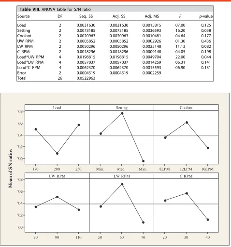
Table VIII. ANOVA table for S/N ratio
Source DF Seq. SS Adj. SS Adj. MS F p-value
Load 2 0.0031630 0.0031630 0.0015815 07.00 0.125
Setting 2 0.0073185 0.0073185 0.0036593 16.20 0.058
Coolant 2 0.0020963 0.0020963 0.0010481 04.64 0.177
UW RPM 2 0.0005852 0.0005852 0.0002926 01.30 0.436
LW RPM 2 0.0050296 0.0050296 0.0025148 11.13 0.082
C RPM 2 0.0018296 0.0018296 0.0009148 04.05 0.198
Load*UW RPM 4 0.0198815 0.0198815 0.0049704 22.00 0.044
Load*LW RPM 4 0.0057037 0.0057037 0.0014259 06.31 0.141
Load*C RPM 4 0.0062370 0.0062370 0.0015593 06.90 0.131
Error 2 0.0004519 0.0004519 0.0002259
Total 26 0.0522963
M
e
an
of
S
N
r
a
ti
os
230 200
170
7.8
7.6
7.4
7.2
7.0
Max. Med.
Min. 8LPM 12LPM 16LPM
110 90
70
7.8
7.6
7.4
7.2
7.0
70 60
50 20 30 40
Load Setting Coolant
UW RPM LW RPM C RPM
Figure 6. Main effects plot (data means) for S/N ratios
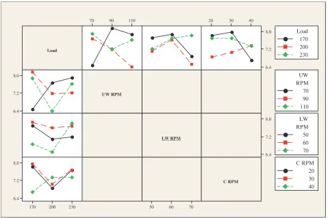
These optimum levels in Table IX were taken as solutions for the causes related to process parameters. Finally, the list of selected solutions is presented in Table X. A risk analysis was carried out to identify any possible negative side effects of the solutions during implementation. The team concluded from the risk analysis that there were no significant negative impacts associated with any of the selected solutions. Hence, an implementation plan was prepared for the above solutions with responsibility and target date for completion for each solution. A time frame of two weeks was provided for implementing these solutions. All the solutions were implemented as per the plan and the results were observed. A graphical presentation of the comparison of results before and after the project is provided in Figure 8.
3.5. Control phase
Load
LW RPM
8.0
7.2
6.4
70 60 50
C RPM UW RPM
110 90
70 20 30 40
8.0
7.2
6.4
8.0
7.2
6.4
230 200 170 8.0
7.2
6.4
Load
230 170 200
UW
110 RPM 70 90
LW
70 RPM 50 60
C RPM
[image:10.594.58.537.66.385.2]40 20 30
[image:10.594.66.532.410.666.2]Figure 7. Interaction plot (data means) for S/N ratios
Table IX. Optimum combination for process parameters
Sl. no. Factor Optimum level
1 Load applied 170
2 Initial load setting Medium
3 Coolant flow rate 12
4 Upper wheel RPM 90
5 Lower wheel RPM 60
6 Cage RPM 30
Table X. Cause–Solution matrix
Sl. no. Cause Solution
1 Repair batches mix up New storage system for repair parts introduced in the process
2 Product family to family variation Process parameters were optimized as per result of DOE 3 Presence of sand blasting dust Cleaning method after sand blasting introduced 4 Material removal rate not OK Reference table prepared for adjusting load
5 Process parameters not OK Optimum factor level combination from DOE
6 Improper setting Optimum factor level combination from DOE
7 Loading/unloading system not OK Conditioning of grinding wheel-loading table is done.
the results are extremely difficult9. Sustainability of the results requires standardization of the improved methods and introduction of monitoring mechanisms for the key results achieved. It also requires bringing awareness among the personnel performing the activities.
Days
P
er
centage
34 31 28 25 22 19 16 13 10 7 4 1 20
15
10
5
0
[image:11.594.139.454.67.294.2]After Before
Figure 8. Rejection percentages—before and after the project
implemented and issued to the corresponding users. As a part of ISO 9001 implementation, once in three months internal audits were carried out in the process. The CTQs of the projects were added to the internal audit checklist so that verifications can be performed during the audits. Control chart is a statistical tool used to monitor a process over time to determine whether special causes of variation occur in the process37. Implementing appropriate control chart can do future monitoring of the process for assignable causes. Since there was a possibility that different types of defects, such as shades, deep line and patches, can appear after grinding, a control chart needs to be introduced for monitoring the process. Since the defect-related data were collected from the process, the most appropriate control chart for this situation was the u chart37. Hence, the u chart was introduced for monitoring the process along with a reaction plan. For every shift, data on number of defects observed during 100% visual inspection were collected and these values were plotted on theuchart by the quality control inspector attached with this process. When any signal for assignable cause appears in the control chart, the quality control inspector discusses this issue with the operator and immediate action was initiated on the process. The reaction plan displayed near to the machine gives direction for identifying the action required for addressing the assignable cause. Also, training was provided for the people associated with the process about the improved operational methods so that they are able to manage the process effectively.
After implementation, the data were compiled from the fine grinding process with respect to the defects for one month and the rejection percentage was found to be 1.19. Hence, as a result of this project, the rejection percentage of the distance pieces at the fine grinding process reduced from 16.6 to 1.19%. The corresponding approximate sigma level was estimated as 3.76. Thus, the sigma level of the process has improved from 2.47 to 3.76. This shows significant improvement in terms of sigma rating as well as defect percentage.
4.
Lessons learned
5.
Managerial implications
There were isolated efforts in the organization in the past to implement initiatives, such as statistical process control, quality circles, continuous improvement programs, Kaizen, 5S and Autonomous maintenance. During the implementation of these initiatives, no systematic effort was made to identify the improvement opportunities in line with business priorities or customer requirements. As a result, the impact of these initiatives was not very visible in the organization whereas in Six Sigma, projects were identified with respect to the voice of the business/customer, and the problems addressed were of highest priority to the organization. Due to success in this project, the management decided to use the Six Sigma methodology for all future improvement initiatives. For monitoring of the Six Sigma initiatives, a core group was formed with all functional heads of the organization. The responsibility of this team was selection of projects and monitoring the execution of projects. All issues related to implementation were also reported to this team for further action. Thus, Six Sigma was introduced as a system in the organization to address any type of problems in the processes. The ultimate objective of the management was to bring a cultural change in the organization by involving everyone in the organization in this movement towards excellence.
6.
Concluding remarks
The Six Sigma method is a project-driven management approach based on the theories and procedures to reduce the defects for a specified process. This paper presents the step-by-step application of the Six Sigma methodology for reducing the rejection level of the fine grinding process. Several statistical tools and techniques were effectively utilized to make inferences during the project.
As a result of the project, the rejection level of distance pieces after the fine grinding process has been reduced to 1.19% from 16.6%. Once the results were observed, with the help of the finance department, the team carried out a cost–benefit analysis for the project. Due to improvement in the process, cost associated with rejection, repair, scrap, re-inspection and tool came down drastically. The annualized savings resulted from this project were estimated and found to be about US$2.4 million. This has given an encouragement for the management to implement the Six Sigma methodology for all improvement initiatives in the organization. Also to encourage the people for participating in the Six Sigma projects, the management declared incentive schemes for the successful teams. In addition to this, during the annual appraisal due weighting was given for individuals who actively participated in the Six Sigma implementation.
Like any other initiative, in Six Sigma also there were inherent difficulties in executing this project. Availability of people for attending training during their busy schedule of day-to-day work was very difficult. Getting support of the people at the lower levels in the organization for participating in the implementation of the solutions was not easy. Since the organization did not have any software for capturing data automatically, collection of data from the process during different phases of the Six Sigma project implementation was also very difficult. The team, by involving people at all levels in the organization, achieved the expected results. Finally, the significant achievement of this project has created many followers for Six Sigma in the organization.
References
1. Snee RD, Hoerl RW.Leading Six Sigma:A Step by Step Guide Based on Experience at GE and Other Six Sigma Companies. Prentice-Hall: New Jersey, 2003.
2. Kumar M, Antony J, Antony FJ, Madu CN. Winning customer loyalty in an automotive company through Six Sigma: A case study.Quality and Reliability Engineering International2007;23(7):849--866.
3. Breyfogle FW.Implementing Six Sigma: Smarter Solutions Using Statistical Methods. Wiley: New York, 1999. 4. Treichler DH. The Six Sigma Path to Leadership. Pearson Education: New Delhi, 2005.
5. Harry M, Schroeder R.Six Sigma:The Breakthrough Management Strategy Revolutionizing the World’s Top Corporations. Doubleday: New York, 1999.
6. Park SH. Six Sigma for productivity improvement: Korean business corporations.Productivity Journal 2002;43:173--183.
7. Pande P, Neuman R, Cavanagh R.The Six Sigma Way:How GE, Motorola and Other Top Companies are Honing their Performance. McGraw-Hill: New York, 2000.
8. Keller PA.Six Sigma Deployment. Quality Publishing House: Arizona, 2001.
9. Gijo EV, Rao TS. Six Sigma implementation—Hurdles and more hurdles.Total Quality Management & Business Excellence2005;16(6):721--725. 10. Pande P, Neuman R, Cavanagh R. The Six Sigma Way Team Field Book: An Implementation Guide for Process Improvement Teams. Tata
McGraw-Hill: New Delhi, 2003.
11. Taghizadegan S.Essentials of Lean Six Sigma. Elsevier: New Delhi, 2006.
12. Goh TN. A strategic assessment of Six Sigma.Quality and Reliability Engineering International 2002;18(5):403--410.
13. Snee RD. Leading business improvement: A new role for statisticians and quality professionals.Quality and Reliability Engineering International 2005;21(3):235--242.
14. Walters L. Six Sigma: Is it really different?.Quality and Reliability Engineering International 2005;21(3):221--224. 15. Montgomery DC. Generation III Six Sigma.Quality and Reliability Engineering International 2005;21(6):iii--iv.
16. Brady M, Allen TT. Six Sigma literature: A review and agenda for future research. Quality and Reliability Engineering International 2006; 22(3):335--367.
17. Hahn GJ. Six Sigma: 20 key lessons learned.Quality and Reliability Engineering International2005;21(3):225--233.
18. Banuelas R, Antony J, Brace M. An application of Six Sigma to reduce waste.Quality and Reliability Engineering International2005;21(6):553--570. 19. Ung ST, Bonsall S, Williams V, Wall A, Wang J. The application of the Six Sigma concept to port security process quality control.Quality and
Reliability Engineering International2007;23(5):631--639.
21. Gijo EV, Scaria J. Reducing rejection and rework by application of Six Sigma methodology in manufacturing process. International Journal of Six Sigma and Competitive Advantage2010;6(1/2):77--90.
22. Lee KL, Wei CC. Reducing mold changing time by implementing Lean Six Sigma. Quality and Reliability Engineering International 2010; 26(4):387--395.
23. Montgomery DC, Runger GC.Applied Statistics and Probability for Engineers (4th edn). Wiley: U.K., 2007. 24. Montgomery DC.Design and Analysis of Experiments(6th edn). Wiley: New York, 2005.
25. Montgomery DC.Introduction to Statistical Quality Control(4th edn). Wiley: New York, 2002.
26. Taguchi G.Systems of Experimental Design, vols 1 and 2. UNIPUB and American Supplier Institute: New York, 1988. 27. Cooper DR, Schindler PS.Business Research Methods. Tata-McGraw Hill: New Delhi, 2006.
28. Bryman A, Bell E.Business Research Methods. Oxford University Press: New Delhi, 2006. 29. Yin RK.Case Study Research: Design and Methods(3rd edn). Sage: California, 2003. 30. Lee TW.Using Qualitative Methods in Organizational Research. Sage: California, 1999.
31. Landis JR, Koch GG. The measurement of observer agreement for categorical data.Biometrics1977;33:159--174.
32. Gijo EV. Improving process capability of manufacturing process by application of statistical techniques.Quality Engineering2005;17(2):309--315. 33. Gijo EV, Perumallu PK. Quality improvement by reducing variation: A case study. Total Quality Management & Business Excellence 2003;
14(9):1023--1031.
34. Phadke MS.Quality Engineering using Robust Design. Prentice Hall: Englewood Cliffs, NJ, 1989. 35. Ross PJ.Taguchi Techniques for Quality Engineering. McGraw-Hill: New York, 1996.
36. Wu CFJ, Hamada M.Experiments—Planning, Analysis, and Parameter Design Optimization. Wiley: New York, 2000. 37. Grant EL, Leavenworth RS.Statistical Quality Control(7th edn). Tata McGraw-Hill: New Delhi, 2000.
38. Juran JM, Godfrey AB.Juran’s Quality Handbook(5th edn). McGraw-Hill International: New York, 2000. 39. Juran JM, Gryna FM.Quality Planning and Analysis(3rd edn). Tata McGraw-Hill: New Delhi, 1995.
Appendix A: Project Charter
Project Title: Reducing rejection in distance pieces after fine grinding process
Background and reasons for selecting the project:
The rejection of distance pieces in the fine grinding process was as high as 16.2%.
Approximately 4200 components are machined during every shift. The cost of
components rejected due to defects was approximately $US1.6 million per annum. In
addition to this, there was loss associated with tool, machine and man-hour related to
rejection of components.
Aim of the project:
To reduce the rejection of distance pieces by 50% after the fine grinding process.
Critical to Quality characteristic:
Rejection percentage of distance pieces after fine grinding process.
Project Scope Fine grinding process
Project Champion: Head - Manufacturing
Project Leader: Senior Manager - Manufacturing
Team Members: Planning Manager, Maintenance Manager,
Quality Control Senior Engineer,
Machine Operator.
Expected Financial Benefits: A saving of approximately $US one million in terms of
reduction in rejection and tool cost.
Expected Intangible Benefits: Reduction in rejection will lead to increased output to
meet the market demand and thereby increase in turnover and reduction in operational expenses.
Expected customer benefits: Improving on time delivery.
Schedule: Define: 2 Weeks, Measure: 2 weeks
Analyze: 3 weeks, Improve: 4 weeks
Appendix B: SIPOC
Supplier Input Process Output Customer
Supplier Pre finished parts
Fine Grinding
Process
Finished parts Assembly Shop
Sand Blasting
Process
Shot blasted parts
Planning
Department
Setting
Parameters
Production
Reports
Manufacturing
Department
Planning
Department
Dressing Method
Planning
Department
CNC Program Quality Reports Quality
Department
Planning
Department
Visual Limit
Sample
Planning
Department
Tooling
Process Steps
Pre-Grinding
Sand Blasting
Fine Grinding
Cleaning & Arranging
Visual Inspection
Authors’ biographies
E. V. Gijo is a Faculty at the Statistical Quality Control and Operations Research Unit of Indian Statistical Institute, Bangalore, India. He holds a Master’s degree in Statistics from M. G. University, Kottayam, Kerala, and a Master’s degree in Quality, Reliability and Operations Research from Indian Statistical Institute, Kolkata. He is an active consultant in the field of Six Sigma, Quality Management, Reliability, Taguchi Methods and allied topics in a variety of industries. He is a certified Master Black Belt and Trainer in Six Sigma and qualified assessor for ISO-9001, ISO-14001 systems. He has published many papers in reputed international journals. He also teaches in the academic programs of the Institute.
Johny Scaria is an Associate Professor in Statistics at Nirmala College, Muvattupuzha, Kerala, India. He holds a Master’s Degree and MPhil in Statistics from Kerala University, and PhD in Statistics from Cochin University of Science and Technology. He has published many papers in reputed international journals. He teaches in the academic programmes of the University. His area of interest includes distribution theory, order statistics and statistical quality control. He is an associate editor of the Journal of the Kerala Statistical Association.