Variable Annuities: Risk Identification and Risk Assessment

City, University of London Institutional Repository

Citation

: Bacinello, A.R., Olivieri, A., Millossovich, P. and Pitacco, E. (2010). Variable

This is the published version of the paper.

This version of the publication may differ from the final published

version.

Permanent repository link:

Link to published version

: CAREFIN Research Paper No. 14/2010

Copyright and reuse:

City Research Online aims to make research

outputs of City, University of London available to a wider audience.

Copyright and Moral Rights remain with the author(s) and/or copyright

holders. URLs from City Research Online may be freely distributed and

linked to.

CAREFIN

Centre for Applied Research in Finance

Working Paper

Universi

tà Co

m

m

erciale

Luigi Bocc

oni

14/2010

Anna Rita Bacinello

Pietro Millossovich

Annamaria Olivieri

Ermanno Pitacco

Variable Annuities: Risk

Identification and Risk

Assessment

by Anna Rita Bacinello Pietro Millossovich

Annamaria Olivieri

Ermanno Pitacco

n. 14/10

Milan, July 2010

Copyright

Carefin, Università Bocconi

INDEX

Abstract II

1. INTRODUCTION 2

2. FROM FIXED BENEFITS TO PACKAGES OF OPTIONS 4

2.1 The traditional deferred life annuity 4

2.2 Adding flexibility 6

2.3 The accumulation period 7

2.4 The decumulation period 9

2.5 Guarantees and options 13

3. THE RISK MANAGEMENT PERSPECTIVE 14

3.1 Why a new approach to actuarial problems 14

3.2 The Risk Management process 15

4. THE STRUCTURE OF VARIABLE ANNUITIES 18

4.1 Benefits, assets, premiums, expenses 18

4.2 Benefits in variable annuities: the contents of GMxB 19

5. VALUATION FRAMEWORK 21

5.1 Benefits in variable annuities: notation and assumptions 21

5.1.1 Guaranteed Minimum Death Benefit 22

5.1.2 Guaranteed Minimum Accumulation Benefit 22

5.1.3 Guaranteed Minimum Income Benefit 23

5.1.4 Guaranteed Minimum Withdrawal Benefit 23

5.2 Valuation 24

5.3 The static approach 24

5.3.1 Cumulated surviving benefits 25

5.3.2 Death benefit 26

5.3.3 Valuation 26

5.4 The dynamic approach 27

5.5 The mixed approach 28

5.6 Comparison 29

6. NUMERICAL INVESTIGATIONS 30

A. THE MONTE CARLO ALGORITHM 33

Abstract*†

Life annuities and pension products usually involve a number of ‘guarantees’, such as, e.g., minimum accumulation rates, minimum annual payments and minimum total payout. Packaging different types of guarantees is the feature of the so-called Variable Annuities. Basically, these products are unit-linked investment policies providing deferred annuity benefits. The guarantees, commonly referred to as GMxBs (namely, Guaranteed Minimum Benefits of type ‘x’), include minimum benefits both in case of death and survival. Following a Risk Management-oriented approach, this paper first aims at singling out all sources of risk affecting Variable Annuities (‘risk identification phase’). Critical aspects arise from the interaction between financial and demographic issues. In particular, the longevity risk may have a dramatic impact on the technical equilibrium of a portfolio. Then, we deal with risk quantification (‘risk assessment phase’), mostly via stochastic simulation of financial and demographic scenarios. Our main contribution is to present an integrated approach to risks in Variable Annuity products, so providing a unifying and innovative point of view.

*We acknowledge financial support from PRIN 2008 research project ‘Retirement saving and private pension benefits: individual choices, risks borne by the providers’.

Anna Rita Bacinello, Pietro Millossovich, Ermanno Pitacco, Department of Business, Economics, Mathematics and Statistics ‘B. de Finetti’ – University of Trieste, Piazzale Europa 1, 34127 Trieste, Italy. Annamaria Olivieri, Department of Economics – University of Parma, Via J.F. Kennedy 6, 43125 Parma, Italy.

1

Introduction

The term variable annuity is used to refer to a wide range of life insurance products, whose benefits can be protected against investment and mortality risks by selecting one or more guarantees out of a broad set of possible arrangements. Originally developed for providing a post-retirement income with some degree of flexibility, nowadays accumula-tion and death benefits constitute important components of the product design. Indeed, the variable annuity can be shaped so as to offer dynamic investment opportunities with some guarantees, protection in case of early death and/or a post-retirement income.

In respect of traditional life insurance products, the main feature of variable annuities is represented by the large variety of possible guarantees, which can be underwritten either for the accumulation, the annuity or the death benefit. The guarantees are briefly referred to as GMxB, Guaranteed Minimum Benefit of type ‘x’, where ‘x’ stands for accumulation (A), death (D), income (I) or withdrawal (W). All GMxB’s provide a protection of the policyholder’s savings account: the GMAB during the accumulation period; the GMDB in case of early death, during the accumulation period and possibly for some years after retirement; the GMIB and the GMWB after retirement, in particular in face of high longevity. Basically, the variable annuity is a fund-linked insurance contract, including a package of financial options on the policy account value (see Smith (1982) and Walden (1985)). Guarantees are then also looked at as riders to the basic benefit given by the account value. A description of the main characteristics of variable annuity products, and the development of the market as well, is provided by Ledlieet al.

(2008).

It is apparent that the design of variable annuities matches features of unit-linked life insurance contracts (namely, the linking mechanism) to those of participating contracts (the guarantees). While the uncertainty in financial markets still makes participating contracts appealing to customers, the increased cost of guarantees has reduced the will-ingness of insurers to deal with such a business; indeed, since guarantees in participating contracts are embedded, and not explicitly selected by the policyholder, traditionally their cost is not charged to the policyholder (when participating contracts were first issued in the Eighties, the embedded guarantees, being deeply out-of-the-money, were meant as a commercial solution). On the other hand, significant advances in hedging techniques enable insurers to offer more sophisticated guarantees, provided that a fee is paid by the policyholder to meet the relevant cost. This is the case for guarantees in variable annuities.

an appropriate approach to the risk management of insurer’s liabilities is required. Some preliminary investigation has been described in this respect. Sun (2006) examines the risks associated with various combinations of guaranteed benefits; Gilbert et al. (2007) describe the findings of a survey on the risk management of guarantees within variable annuity products in the US. More work is required in this perspective, in particular within an Enterprise Risk Management perspective.

Among the several phases of the risk management process, the pricing and hedg-ing of guarantees, i.e. of the relevant financial options, should be a major concern for the insurer when designing the contract. It is worthwhile to point out that, simi-larly to participating or unit-linked contracts, financial options in variable annuities are non-standard, as their exercise depends not just on economic factors, but also on the survival or death of the insured (when the guarantees relate to accumulation, death or withdrawal benefits), or on preferences in regard of the trade-off between annuitisation and bequest (when the guarantee concerns the choice of the post-retirement income). Thus, appropriate evaluation techniques need to be developed, which allow one to ac-count on one hand for the interaction between financial and mortality issues, on the other for policyholder behaviour.

Possible approaches to the pricing and hedging of the most common guarantees in variable annuity arrangements have already been discussed in the literature. Recently, special attention has been addressed to withdrawal benefits, thanks to the fact that, when appropriately managed, they can provide a flexible pension payment. With regard to the pricing of this class of benefits, Milevsky and Salisbury (2006) assess their cost

and compare their findings with prices quoted in the market; Dai et al. (2008) develop

a singular stochastic control model, and investigate the optimal withdrawal strategy for a rational policyholder; Chen and Forsyth (2008) describe an impulse stochastic control formulation, while Chen et al. (2008) explore the effect of alternative policyholder be-haviours. In all such contributions, most of the attention is devoted to financial risks. Mortality is addressed, e.g., by Milevsky and Posner (2001), dealing with the pricing of guaranteed minimum death benefits; as they look for closed formulae, a simplified as-sumption is adopted for the force of mortality, resulting in some drastic approximations. The valuation of a variable annuity providing a guaranteed minimum death benefit and a guaranteed minimum withdrawal is the target of Bélangeret al.(2009), while a general framework for the pricing of guarantees under the assumption of optimal policyholder

behaviour is suggested by Bauer et al. (2008).

terminology is rather fanciful and sometimes ambiguous. So, in Section 4 we provide a detailed description of the most common guarantees. We refer to contributions avail-able in the literature (in particular, to Ledlieet al.(2008)), and to insurers’ informative material. Then, we investigate pricing and hedging issues of some guarantees, mod-elling jointly several risk sources. We adopt a valuation model developed by Bacinello

et al. (2010), which allows for a comprehensive representation of financial and mortality risks. The model is described in Section 5; in Section 6 we discuss its implementation. We focus in particular on the withdrawal benefit since it can provide a flexible pension payment (when appropriately managed), and because it is currently available only in variable annuities (conversely, death, accumulation and income benefits, in some forms, are provided also by traditional products).

2

From fixed benefits to packages of options

In the Nineteenth century a large variety of policies, to some extent tailored on the personal insured’s needs, was customary in several European insurance markets. Later, a ‘standardization’ process started, with a progressive shift to a very small set of standard products, mainly consisting of the classical endowment insurance, the term insurance, the immediate life annuity, and the deferred life annuity.

It is worth noting that, to some extent, an inverse process is currently developing. Indeed, many modern insurance policies are designed as ‘packages’, whose items may be either included or not in the product actually purchased by the client.

Interesting examples are provided by insurance policies which eventually aim at constructing a post-retirement income. These products witness the shift from traditional deferred life annuities to more complex packages consisting of (see Figure 1):

– one or more insurance (or financial) products for the ‘accumulation’ phase, namely

the working period of the policyholder;

– an insurance (or financial) product for the ‘decumulation’ phase, namely the

post-retirement period.

Variable annuities can be placed in this framework. While a detailed description of these products is provided in Section 4.2, we now introduce the actuarial aspects of insurance contracts aiming to provide benefits extending over a long spell of the individual lifetime. We recall that premium calculation is traditionally based on the equivalence principle. Thus, the single premium of an insurance policy, according to a traditional approach, is simply given by the expected present value of the benefits. For further details, the reader can refer to Pitacco et al. (2009).

2.1

The traditional deferred life annuity

Vt

time

fu

n

d

/

re

se

rve

T-1 T A

T+1

1 0 2

age

x+T x

DECUMULATION ACCUMULATION

annuity benefits / withdrawals premiums /

savings

Figure 1: Accumulation and decumulation phase

Consider a deferred life annuity of one monetary unit per annum, with a deferred

period of T years, which coincides with the accumulation period. Let x denote the age

at the beginning of the accumulation process, i.e. at time 0. Assume that each annual

payment is due at the beginning of the year (that is, in advance). The actuarial value at time0, T|ax¨ (according to the common actuarial notation), is given by

T|¨ax = ∞

X

h=T

(1 +i)−h_{hpx, (2.1)}

where i denotes the technical interest rate and hpx is the probability of an individual

age x being alive at age x+h.

The deferred annuity can be financed, in particular, via a sequence ofT annual level premiums, paid at times0,1, . . . , T ₋1. The annual level premiumP for a deferred life

annuity ofI monetary units per annum, according to the equivalence principle, is given

by

P =I T|ax¨ ¨ ax:T⌉

,

where

¨ ax:T⌉=

T−1

X

h=0

(1 +i)−h_{hpx. (2.2)}

Two important aspects of the actuarial structure of deferred life annuities financed by annual premiums should be stressed.

or even more. Further, the life table underlying the probabilities hpx should keep its validity throughout the same period. Although these probabilities are drawn from a projected life table, the future trend of mortality is unknown, so that the longevity risk arises.

b. If the policyholder dies before time T, no benefit is due. This is, of course, a

straight consequence of the policy structure, according to which the only benefit is the deferred life annuity.

Feature (b) is likely to have a negative impact on the appeal of the annuity product. However, the problem can be easily removed by adding to the policy a rider benefit such as the return of premiums in case of death during the deferred period, or including some

death benefit with term T (see Sections 2.2 and 2.4).

The problems pointed out in (a) are much more complex, and require a rethinking of the whole structure and design of the life annuity product. A first step toward structures more flexible than the traditional deferred life annuity financed by annual level premiums is described below.

The severity of the longevity risk borne by the life annuity provider can be weakened if the annuity purchase is arranged according to a single-recurrent premium scheme. In this case, with the premium Ph paid at time h (h = 0,1, . . . , T ₋1) a deferred life

annuity of annual amount Ih, with deferred period T ₋h, is purchased. In actuarial

terms:

Ph =Ih T−h|¨a[

h]

x+h. (2.3)

Note that the actuarial value T−h|¨a[

h]

x+h is calculated according to the technical basis adopted at time h. Hence, the total annuity benefit I, given by

I = T−1

X

h=0

Ih,

is ultimately determined and guaranteed at timeT ₋1only. According to this

step-by-step procedure, the technical basis, used in (2.3) to determine the amountIh purchased

with the related premiumPh, can change every year, thus reflecting possible adjustments in mortality forecasts.

2.2

Adding flexibility

To build-up a more general framework, we now address separately the accumulation phase and the decumulation phase, and focus on insurance and financial products which can constitute the building blocks of more general policies covering the two phases.

Flexibility in insurance products can be achieved following various ways. In partic-ular:

– instead of fixed benefits, the insurance policy can provide benefits linked to

– various policyholder’s options can be included in the policy conditions;

– several types of benefits (that is, benefits in case of death and survival) can be

packaged in the same insurance contract.

Of course, these approaches to flexibility can be implemented in both the accumulation and the decumulation phase. A first look at flexibility mechanisms is provided by Figures 2 and 3, whereas a more detailed discussion follows in Sections 2.3 and 2.4.

FLEXIBILITY in the ACCUMULATION PHASE

Unit-linked

Variable Life

Universal Life

Insured's options

Linking Benefit Packaging

Participating

Figure 2: Products embedding flexible features: the accumulation phase

2.3

The accumulation period

The deferred life annuity, as described in Section 2.1, can be seen as a pure endowment taken out at agexwith maturity at agex+T, followed (in case of survival at maturity) by an immediate life annuity with benefits due at the beginning of each year. In formal terms, from (2.1) we obtain

T|ax¨ = (1 +i)−TTpx

∞

X

h=0

(1 +i)−h_hpx

+T =TEx¨ax+T, (2.4)

where TEx = (1 +i)−TTpx denotes the actuarial value of a pure endowment with a

unitary insured amount.

FLEXIBILITY in the DECUMULATION PHASE

Linking Insured's options

Immediate life annuity

Income drawdown

Staggered annuitization

Capital Protection

Enhanced Pension (LTC)

Benefit Packaging

Unit-linked

Participating Last survivor _annuity

Figure 3: Products embedding flexible features: the decumulation phase

Conversely, a pure endowment can be used to pursue the accumulation target, then converting the maturity benefit into an immediate life annuity. The pure endowment can be replaced by a purely financial accumulation, via appropriate saving instruments. The loss in terms of the mutuality effect is very limited as just the working period (or part of it) is concerned. Hence, a very modest extra-yield (compared to the interest rate in the pure endowment) can replace the so-called mortality drag. See Pitaccoet al.

(2009), also for numerical examples.

Of course, alternative insurance products including a benefit in case of life at time

T can replace the pure endowment throughout the accumulation period. Examples are

given by the traditional endowment insurance policy, by various types of unit-linked endowments, and so on. In many cases, some minimum guarantee is provided: for example, the technical rate of interest in traditional products like pure endowments and endowment insurances, a minimum death benefit and/or a minimum maturity benefit in unit-linked contracts.

More complex products can be built-up including options and packaging benefits. For example, the so-called ‘Variable Life’ insurance allows the policyholder to vary the amount of periodic premiums, whereas the ‘Universal Life’ policies can also include payments other than the death benefit, like sickness payments, lump sum in the case of permanent disability, and so on.

Whatever the insurance product may be, the benefit at maturity can be used to purchase an immediate life annuity. However, the ‘quality’ of the accumulation product can be improved, from the perspective of the policyholder, including in the product itself an ‘option to annuitise’. This option allows the policyholder to convert the lump sum at maturity into an immediate life annuity, without the need to cash in the sum and pay the expense charges related to the underwriting of the life annuity.

the adverse selection risk, as the policyholders who choose the conversion into a life annuity will presumably be in good health, with a life expectancy higher than average. However a further risk arises, due to the uncertainty in future mortality trends, i.e. the longevity risk (as already noted in Section 2.1).

If the annuitisation rate, that is the quantity _¨ax1

+T which is applied to convert the

maturity benefit into an immediate life annuity, is stated (and hence guaranteed) only at maturity, the time interval throughout which the insurer bears the longevity risk clearly coincides with the time interval during which the life annuity is paid.

However, more ‘value’ can be added to the product if the annuitisation rate is guaran-teed during the accumulation period, the limiting case being represented by the annuiti-sation rate guaranteed at time 0, i.e. at policy issue. This case is known as Guaranteed Annuity Option (GAO). Then, the GAO provides the policyholder with the right to receive at retirement either a lump sum (the maturity benefit) or a life annuity whose annual amount is calculated at a guaranteed rate. The GAO will likely be exercised

by the policyholder if the annuity rate applied by the insurer at time T for pricing

immediate life annuities will be lower than the guaranteed one.

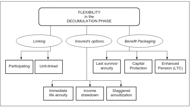
2.4

The decumulation period

Also in the decumulation phase flexibility can be achieved both by allowing the poli-cyholder to exercise various options and by linking the annuity benefits to investment performance. Further, various features can be packaged into the life annuity product. Figure 3 illustrates possible flexibility in the decumulation phase.

First, at the end of the accumulation period, a range of alternatives can be proposed to the retiree. The following ones are of practical interest:

i. an immediate life annuity, typically provided by an insurer;

ii. a drawdown process, namely a sequence of withdrawals from a fund managed by a financial intermediary (an insurer, in particular);

iii. a ‘staggered annuitisation’, that is

– a temporary drawdown process (say, for 5 years);

– then, one or more partial annuitisations of the residual fund, so that the

post-retirement income is partly provided by the non-annuitised fund, and partly by the purchased life annuities;

clearly, the staggered annuitisation is a mixture of alternatives (i) and (ii).

These alternatives can be compared in terms of risks borne, on the one hand, by the financial intermediary (the insurer, in particular) and, on the other, by the retiree.

paid throughout the whole lifetime. As regards the life annuity provider, we note that, if the actual lifetimes of the annuitants lead to numbers of survivors greater than the estimated ones, then the mutuality mechanism can finance only part of the payments to annuitants still alive, whereas the uncovered part constitutes a loss for the annu-ity provider. Conversely, numbers of survivors less than the estimated ones lead to a provider’s profit. Thus, the annuity provider takes risks related to the longevity of the annuitants.

If the post-retirement income is obtained by withdrawals from the fund, in principle no risk related to the lifetime is borne by the financial intermediary. Conversely, the retiree takes the risk of outliving the available resources, as the drawdown process can exhaust sooner or later the fund (provided that the annual withdrawal is greater than the annual interest). On the contrary, in the case of early death of the retiree, the residual amount will be available as a bequest. However, as we will see in Section 4.2, specific policy conditions can provide guarantees in respect of the duration of the drawdown process.

We now describe some basic models of immediate annuity (focussing on annuities in arrears only), among which we find:

– the straight life annuity;

– life annuities which combine two or more benefits, and thus can be considered as

(traditional) packages of benefits.

Let us denote with T the starting point of the decumulation period, and withx+T

the annuitant’s age. Let A denote the amount, available at time T, to finance the life

annuity (we note that, in the case of the deferred life annuity described in Section 2.1,

A is given by the mathematical reserve at time T of the annuity itself). The relation

between A and the annual payment I depends on the policy conditions which define

the (random) number of payments, and hence the duration of the decumulation period. The following cases are of practical interest.

1. If the number of annual payments, saym, is stated in advance, we have an annuity-certain, i.e. a simple withdrawal process. Then, the annual benefit I[1] _{is defined}

by the following relation:

A =I[1]am⌉.

2. In the case of a whole life annuity, the annual payments stop upon the annuitant’s death. We have:

A=I[2]ax+T.

3. The m₋year temporary life annuity pays the annual benefit while the annuitant

survives during the first m years. Then

A=I[3]ax+T:m⌉=I[3]

m X

h=1

(1 +i)−h_hpx

Of course,I[3] > I[2].

4. If the annuitant dies soon after time T, neither the annuitant nor the annuitant’s estate receive much benefit from the purchase of the life annuity. In order to mitigate this risk, it is possible to buy alife annuity with a guarantee period (5 or 10 years, say), in which case the benefit is paid for the guarantee period regardless of whether the annuitant is alive or not. Hence, for a guarantee period ofm years we have

A=I[4]am⌉+I[4]m|ax+T. Clearly, we find I[4] < I[2].

We have so far assumed that the annuity payment depends on the lifetime of one individual only, namely the annuitant. However, it is possible to define annuity models involving two (or more) lives. Some examples (referring to two lives) follow.

5. Consider an annuity payable as long as at least one of two individuals (the

an-nuitants) survives, namely a last-survivor annuity. Let now denote by y and z

respectively the ages of the two lives at the annuity commencement. The actuar-ial value of this annuity is usually denoted by ay,z, and can be expressed as

ay,z =a(1)y +a(2)z −ay,z,

where the suffices(1),(2)denote the life tables (for example, referring to males and females respectively) used for the two lives, whereasay,z denotes the actuarial value of an annuity of 1 per annum, payable while both individuals are alive (namely a

joint-life annuity). Hence,

A=I[5]ay,z =I[5](a(1)_y +a(2)_{z −}ay,z). (2.5)

Of course, I[5] < I[2]. Note that, if we accept the hypothesis of independence between the two random lifetimes, we have

ay,z =

∞

X

h=1

(1 +i)−h_hp(1)

y hp(2)z .

In (2.5) it has been assumed that the annuity continues with the same annual amount until the death of the last survivor. A modified form provides that the amount, initially set to I[5]_{, will be reduced following the first death: toI}[5]′ _{if the}

individual (2) dies first, and toI[5]′′ if the individual (1) dies first. Thus

A=I[5]′a(1)_y +I[5]′′a_z(2)+ (I[5] ₋I[5]′₋I[5]′′)ay,z, (2.6)

6. A reversionary annuity (on two individuals) is payable while a given individual, say individual (2), is alive, but only after the death of the other individual. Such an annuity can be used, for example, as a death benefit to be paid to a surviving spouse or dependant (and thus constitutes a ‘settlement’ option).

We note that some policy conditions provide a ‘final’ payment, namely some benefits after the death of the annuitant. In particular, thecomplete life annuity (or apportion-able annuity) is a life annuity payable in arrears which provides a pro-rata adjustment on the death of the annuitant, consisting in a final payment proportional to the time elapsed since the last payment date. Clearly, this feature is more important if the annuity is paid annually, and less important in the case of, say, monthly payments.

Capital protection represents an interesting feature of some annuity policies, usually called value-protected annuities, and actually represents a traditional packaging of ben-efits. Consider, for example, a single-premium life annuity. In case of early death of the annuitant, a value-protected annuity will pay to the annuitant’s estate the difference (if positive) between the single premium and the cumulated benefits paid to the annuitant. Usually, capital protection expires at some given age (75, say), after which nothing is paid even though the difference above mentioned is positive. The capital protection benefit can be provided in two ways:

– in a cash-refund annuity the balance is paid as a lump sum;

– in an instalment-refund annuity the balance is paid in a sequence of instalments.

Adding capital protection clearly reduces the annuity benefit (for a given single pre-mium).

As regards the time profile of the annuity benefit, the following classification reflects the life annuity types offered in various insurance markets.

Level annuities (sometimes called standard annuities) provide an income which is constant in nominal terms. Thus, the payment profile is flat.

A number of models of ‘varying’ annuities have been derived, mainly with the purpose of protecting the annuitant against the loss of purchasing power because of inflation. Many models can be interpreted as tools to add flexibility to the life annuity product (see models (b) to (f) below). First, we focus onescalating annuities.

(a) In thefixed-rate escalating annuity (orconstant-growth annuity) the annual benefit increases at a fixed annual rate, say c, so that the sequence of payments is

I1, I2 =I1(1 +c), I3 =I1(1 +c)2, . . . .

The premium is calculated accounting for the annual increase in the benefit. Thus, for a given single premium of the immediate life annuity, the starting benefit I1 is

lower than the benefit the annuitant would get from a level annuity.

Various types of index-linked escalating annuities are sold in annuity and pension

(b) Inflation-linked annuities provide annual benefits varying in line with some index, for example a retail-price index (like the RPI in the UK), usually with a stated upper limit. An annuity provider should invest the premiums in inflation-linked assets so that these back the annuities with payments linked to a price index.

(c) Equity-indexed annuities earn annual interest that is linked to a stock or other equity index (for example, the Standard & Poor’s 500). Usually, these annuities promise a minimum interest rate.

Moving to investment-linked annuities, we focus on the following models.

(d) In a with-profit annuity the single premium is invested in an insurer’s with-profit

fund. Annual benefits depend on anassumed annual bonus rate (e.g. 5%), and on

the sequence of actual declared bonus rates, which in turn depend on the

perfor-mance of the fund. In each year, the annual rate of increase in the annuity depends on the spread between the actual declared bonus and the assumed bonus. Clearly, the higher is the assumed bonus rate, the lower is the rate of increase in the an-nuity. The benefit decreases when the actual declared bonus rate is lower than the assumed bonus rate. Although the annual benefit can fluctuate, with-profit annuities usually provide a guaranteed minimum benefit. This kind of policies is very common in the UK market.

(e) Various profit participation mechanisms (other than the bonus mechanism

de-scribed above in respect of with-profit annuities) are adopted in many European continental countries. A share (e.g. 80%) of the difference between the yield from the investments backing the mathematical reserves and the technical interest rate (i.e., the minimum guaranteed interest, say 2% or 3%) is credited to the reserves. This leads to increasing benefits, thanks to the extra-yield.

(f) The single premium of aunit-linked life annuity is invested into unit-linked funds. Generally, the annuitant can choose the type of fund, for example medium risk managed funds, or conversely higher risk funds. Each year, a fixed number of units are sold to provide the benefit payment. Hence, the benefit is linked directly to the value of the underlying fund, and then it fluctuates in line with unit prices. Some unit-linked annuities, however, work in a way similar to with-profit annuities. An annual growth rate (e.g. 6%) is assumed. If the fund value grows at the assumed rate, the benefit stays the same. If the fund value growth is higher than assumed, the benefit increases, whilst if lower the benefit falls. Some unit-linked funds guarantee a minimum performance in line with a given index.

2.5

Guarantees and options

features is beyond the scope of this paper. An exhaustive description of guarantees and options in variable annuity products will be provided in Section 4. Here we just address some issues.

– The guarantee of fixed life and death benefits means that, whatever the numbers

of people dying and surviving in the portfolio, the insurer takes the risk of paying the amounts stated in the policy conditions.

– The expression minimum benefit guarantees denotes a wide range of guarantees

which applies to unit-linked benefits.

– Surrender and alterations constitute policyholder’s options which imply a change in future benefit cash flows with respect to flows initially stated in the policy.

– The option to annuitise has been already discussed in the previous sections (in particular, see Section 2.3); notwithstanding, it is worth stressing that this option constitutes a critical feature in insurance products which aim at providing post-retirement income, in particular as regards the longevity risk.

All the options and guarantees embedded in an insurance product should be carefully accounted for in both the pricing and the reserving steps, with an appropriate assessment of the risks involved. It follows that the traditional equivalence principle, yet widely adopted in life insurance calculations, reveals several weak points when options and guarantees have to be assessed. A risk-management approach should then be adopted, in order to properly deal with the risks borne by the insurer (and by the annuity provider in particular) as a consequence of the guarantees and options included in the insurance package.

3

The Risk Management perspective

3.1

Why a new approach to actuarial problems

Advantages provided by ‘large’ portfolio sizes in respect of the risk originated by mortal-ity random fluctuations, namely the ‘volatilmortal-ity’ or process risk, justify, to some extent, the traditional approach adopted in life insurance actuarial calculations, mainly based on the equivalence principle. However, it is worth noting the following aspects.

– Other sources of risk also affect the results of a life insurance portfolio such as market (or investment) risk, expense risk, credit risk, lapse risk, etc..

– The presence of other mortality risk components should be recognized. In

LIFE

INSURANCE

POLICY

GUARANTEES _{(& GUARANTEES)} OPTIONS

Fixed rider benefits (accident, sickness, etc)

Cliquet structure in participation mechanisms Fixed life and death benefits

"Minimum" benefit

guarantees _Switching options Change in premium level Option to annuitise Insurability guarantee

Surrender

Alterations

Settlement options

Figure 4: The life insurance policy as a package of guarantees and options

– The process component of mortality risk should be anyway accounted for, in

par-ticular when small insurance portfolios (or pension plans) are addressed.

– The impact of both mortality and investment risks can be rather high in the

presence of some guarantees and options. This happens, in particular, in variable annuity products, as we will see in Section 4.

Each source of risk (mortality, yield from investment, and so on) should be investigated by singling out its components and other relevant factors (for example the portfolio size, the prevailing type of products, and so on). With these arguments in mind, we move towards a risk-management oriented approach to life insurance technical problems. Actually, the ‘identification’ of risks constitutes the first step of the Risk Management (RM) process.

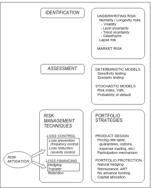
3.2

The Risk Management process

IDENTIFICATION

ASSESSMENT

UNDERWRITING RISK Mortality / Longevity risks - Volatility

- Level uncertainty - Trend uncertainty - Catastrophe Lapse risk . . . MARKET RISK . . . DETERMINISTIC MODELS Sensitivity testing Scenario testing STOCHASTIC MODELS Risk index, VaR, Probability of default . . . RISK MANAGEMENT TECHNIQUES LOSS CONTROL Loss prevention (frequency control) Loss reduction (severity control) LOSS FINANCING Hedging Transfer Retention PORTFOLIO STRATEGIES PRODUCT DESIGN Pricing (life table, guarantees, options, expense loading, etc) Participation mechanism

PORTFOLIO PROTECTION Natural hedging

Reinsurance, ART No advance funding Capital allocation

RISK MITIGATION

Figure 5: The risk management process

RM process applied to life insurance. For further detail, the reader can refer to Pitacco

et al. (2009).

Theidentification of risks affecting an insurer can follow, for example, the guidelines provided by IAA (2004) or those provided within the Solvency 2 project (see CEIOPS (2007), CEIOPS (2008)). For life insurance products, mortality/longevity risk (and the related components) and market risk can have dramatic impact on portfolio results.

The risk assessment step can be performed, at least in principle, by using both de-terministic and stochastic models. Dede-terministic models allow us to calculate the range of values that some output variables (for example: cash flows, profits, mathematical reserves) may assume in respect of the values attributed to some input variables, but do not yield any probabilistic evaluation related to output variables (for example: the probability distribution, variance, Value at Risk, default probability, and so on).

frame-work, a rigorous assessment of a number of risks (mortality/longevity and market risks in particular) requires the use of stochastic models. Usually, the complexity of the as-sessment problems requires the adoption of Monte Carlo simulation techniques. Some implementations concerning variable annuity products are presented in Section 6.

Finally, risk management techniques for dealing with risks inherent in a life

insur-ance portfolio include a wide set of tools which can be interpreted, under an insurinsur-ance perspective, as portfolio strategies aimed at risk mitigation.

We just focus on some critical aspects, which should be carefully considered when managing a life insurance portfolio. For further aspects, the reader can refer to Pitacco

et al. (2009). The product design obviously constitutes the starting point of portfolio strategies. As regards variable annuities and the guarantees therein included, the reader should refer to Section 4.

When dealing with insurance products as bundles of guarantees and options (see Figure 4), some crucial points can be immediately singled out. In particular, we stress the following points.

1. The choice of the life table can mitigate the risk of losses due to the payment of life and death benefits whose amount is guaranteed whatever the mortality in the portfolio may be.

2. The structure of profit participation can be weakened with respect to the cliquet mechanism, so as to lower the level of market risk borne by the insurer.

3. Any minimum guarantee included in the policy conditions requires a sound pricing (relying, of course, on appropriate stochastic models).

4. ‘Natural’ hedging, in the context of life insurance, refers to diversification strategies combining opposite benefits with respect to life duration. The main idea is that, if mortality rates decrease, then life annuity costs increase while death benefit costs decrease (and vice versa). Natural hedging can be implemented in two ways.

(a) Hedging across time is pursued by packaging survival benefits and death benefits in the same insurance policy. An example is provided by capital protection (the death benefit) in a life annuity product (the survival benefit); see Section 2.4.

4

The structure of variable annuities

4.1

Benefits, assets, premiums, expenses

As mentioned in Section 1, variable annuities merge the most attractive commercial features of unit-linked and participating life insurance contracts: dynamic investment opportunities, protection against financial risks and benefits in case of early death. Further, they offer modern solutions in regard of the post-retirement income, trying to arrange a satisfactory trade-off between annuitisation needs and bequest preferences. Basically, the variable annuity is a fund-linked insurance contract, with rider benefits in the form of guarantees on the policy account value; such riders become attainable either in case of death or survival.

Available guarantees may be first classified into two main broad classes:

– Guaranteed Minimum Death Benefits (GMDB);

– Guaranteed Minimum Living Benefits (GMLB).

The second class can be further arranged into three subclasses:

– Guaranteed Minimum Accumulation Benefits (GMAB);

– Guaranteed Minimum Withdrawal Benefits (GMWD);

– Guaranteed Minimum Income Benefits (GMIB).

As already mentioned in Section 1, guarantees in variable annuities are referred to as GMxB, where ‘x’ stands for the class of benefits involved: accumulation (A), death (D), withdrawal (W) or income (I). In Section 4.2 we provide a general description of the contents of each GMxB, whilst in Section 5.1 we formalize some specific examples.

Variable annuities are generally issued with single premium or single recurrent pre-miums. The total amount of premiums is also named the principal of the contract or the invested amount. Apart from some upfront costs, premiums are entirely invested into the reference funds chosen by the policyholder. Several investment opportunities are available to the customer, providing different risk-return profiles. Thus, the policy-holder can opt for more conservative or more dynamic asset combinations. She is also allowed to switch from one risk-return solution to another at no cost, if some constraints are fulfilled (for example, the switch is required no more than once a year). Unlike in with-profit or participating business, reference funds backing variable annuities are not required to replicate the guarantees selected by the policyholder, as these are hedged by specific assets. Therefore, reference fund managers have more flexibility in catching investment opportunities.

at policyholder’s discretion, when the contract is already in-force. Accordingly, the corresponding fees start or stop being charged. The cost of guarantees, as well as other expenses, are typically expressed as a given percentage of the policy account value. In particular when relating to mortality or longevity guarantees, applying a constant percentage may result in some drastic approximations of the fair underlying cost, as it emerges in Section 6, where the cost of the guarantees is investigated.

4.2

Benefits in variable annuities: the contents of GMxB

In this section we provide some details on the contents of each GMxB.

The Guaranteed Minimum Accumulation Benefit_{(GMAB) is usually}

avail-able prior to retirement. At some specified date, the insured (if alive) is credited the greater between the policy account value and a guaranteed amount. Such guaranteed amount can be stated as follows:

– the amount of premiums paid, net of partial withdrawals;

– the roll-up of premiums, net of partial withdrawals, at a specified guaranteed

interest rate;

– the highest account value recorded at some specified times (prior to the maturity

of the GMAB); this is the so-called ratchet guarantee, which locks-in the positive performances of the reference fund.

A further guarantee which may be attached to the GMAB is the reset, which gives the opportunity to renew the GMAB when it reaches maturity.

Similarly to the GMAB, also theGuaranteed Minimum Death Benefit_(GMDB)

is available during the accumulation period; some insurers are willing to provide a GMDB also after retirement, up to some maximum age (say, 75 years). The structure of the guarantee is similar to the GMAB: in case of death prior to the stated maturity, the insurer will pay the greater between the account value and a stated amount. The guar-anteed amount can be either fixed, e.g. equal to

– the amount of premiums paid, net of partial withdrawals;

– the roll-up of premiums, net of partial withdrawals, at a specified guaranteed

interest rate;

or depending on the account value, such as

– the highest account value recorded at some specified times prior to death (ratchet);

– the account value at some prior specified date (the so-called reset date1_{) plus the}

total amount of premiums paid following such date, net of partial withdrawals.

1

The difference between the ratchet and the reset guarantee within the GMDB stands in the behaviour of the guaranteed minimum amount: in the ratchet guarantee the minimum amount never decreases, whilst a reduction may occur in the reset, if the account value decreases between two reset dates.

TheGuaranteed Minimum Income Benefit_{(GMIB) provides a lifetime annuity}

from a specified future point in time. The guarantee may be arranged in two different ways:

– the amount to be annuitised will be the greater between the account value and a

specified sum. Possible ways to specify such an amount are similar to the GMAB. The annuitisation rate will be defined according to market conditions prevailing at the annuitisation date;

– the annuitisation rate will be the more favourable between a stated rate and what

resulting from current conditions. The annuitised amount will be the account value. Thus, this case is similar to a Guaranteed Annuitisation option (GAO).

The former guarantee is sometimes described as a guarantee on the annual amount, which would suggest an arrangement similar to a deferred life annuity; it is then worth-while to stress that the guarantee actually concerns the amount to be annuitised, as described above. After annuitisation, the policyholder loses access to the account value (while prior to annuitisation the contract works like an investment product, bearing some guarantees). The guarantee must be selected by the policyholder some years be-fore annuitisation; typically, the GMIB may be exercised after a waiting period of 5 to 10 years. The cost of the GMIB is deducted from the account value during the ac-cumulation period. If prior to annuitisation the policyholder gives up the guarantee, the insurer stops deducting the relevant fee. Typically, full annuitisation is required; however, partial annuitisation is admitted in some arrangements. As far as the duration of the annuity is concerned, the following solutions are usually available: a traditional life annuity; a reversionary annuity; a life annuity with a minimum number of payments (say, up to 5 or 10 years). Money-back arrangements may also be available, providing a death benefit consisting of the residual principal amount, i.e. the annuitised amount net of the annual payments already cashed. The annual amount may be either fixed, participating or indexed to inflation or stock prices; a financial risk is borne by the annuitant in the latter case, as the annual amount can fluctuate in time (conversely, in a participating scheme the annual amount never decreases).

The Guaranteed Minimum Withdrawal Benefit _{(GMWB) guarantees}

or limited to some years (e.g., 10 years). Note that, thanks to the ratchet, the guaran-teed annual payment may increase in time; in some arrangements, a maximum accepted annual increase is stated in policy conditions. The guaranteed annual payment may be alternatively meant as the exact, the maximum or the minimum amount that the policyholder is allowed to withdraw in each year. In the last case, any withdrawal above the guaranteed level reduces the base amount. The duration of the withdrawals may be fixed (e.g., 20 years) or lifetime. In the former case, if at maturity the account value is positive, it is paid back to the policyholder or, alternatively, the contract stays in-force until exhaustion of the policy account value. The cost of the guarantee is deducted from the account value during the payment period; if the policyholder gives up the guaran-tee, the relevant fee stops being applied. During the withdrawal period, the policyholder keeps access to the unit-linked fund; if at death the account value is positive, such an amount is paid to the estate of the policyholder.

From the descriptions above, it emerges that GMAB and GMDB are similar to what can be found in investment life insurance contracts, apart from the possible range of guarantees, which is wider in variable annuities than in traditional contracts. The GMIB is like a traditional life annuity, possibly participating. The GMWB is the real novelty of variable annuities in respect of traditional life insurance contracts; it provides a benefit which is similar to an income drawdown, but with guarantees. When comparing a GMIB to a GMWB, three major differences arise: the duration of the annuity (which is lifetime in the GMIB), the accessibility to the account value (just for the GMWB) and the features of the reference fund (which is unit-linked in the GMWB, but typically participating in the GMIB). Clearly, the presence of death benefits also in the GMIB, a lifetime duration for the withdrawals in the GMWB and other possible features reduce a lot the differences between the GMIB and the GMWB. Apart from the use of one name or the other, policy conditions should suggest the real features of the income provided by the contract.

5

Valuation framework

In this section we give some detailed examples of GMxB’s and provide a formalization suitable to assess the cost of the guarantees under quite general model assumptions.

5.1

Benefits in variable annuities: notation and assumptions

We consider a single premium variable annuity contract issued at time0. Let P denote

the single premium and T _≥0 the end of the accumulation period.2 _{We only consider}

single premium contracts as they constitute the building block for single recurrent

pre-mium schemes. We denote by At the policy account value at time t. Clearly, this value

depends on the evolution of the reference fund in which the single premium is invested.

2

We assume that all possible guarantees are selected at time 0 and are kept for all the contract duration. The main guarantees offered by the contract can be formalized as follows.

5.1.1 Guaranteed Minimum Death Benefit

In case of death at time t, during the accumulation period (i.e. t _≤ T), the benefit is given by

max_{At, GD_t}, t_≤T, (5.1)

where GD

t is some guaranteed amount such as, e.g.,

GD_t =P (return of premium) (5.2)

GD_t =Peδt_{, δ >0 (roll-up) (5.3)}

GD_t = max ti<t

Ati (ratchet) (5.4)

GD_t = max

Peδt,max ti<t

Ati

(ratchet + roll-up) (5.5)

GD_t =Amax{ti:ti<t} (reset). (5.6)

Equation (5.2) describes a simple return of premium guarantee, while (5.3), that

en-compasses (5.2), describes a roll-up guarantee, where δ is the guaranteed continuously

compounded interest rate. Clearly (5.3) could be modified to accomodate a time de-pendent deterministic guaranteed interest rate; this would allow us to model situations in which the roll-up feature applies only until a given age of the insured and/or the rate is adjusted at regular intervals. We mention that if the policyholder withdraws

funds from her account during the accumulation period, the guaranteed amount GD

t is reduced accordingly. Equation (5.4) describes a ratchet guarantee, where the profits on the reference fund are locked-in at the (predetermined) ratchet dates t0, t1, ..., tn, with

0 = t0 < t1 < ... < tn < T. Equation (5.5) describes a combination of roll-up and

ratchet features. Equation (5.6) describes the reset guarantee, where t1, t2, ..., tn now

define the reset dates. Further definitions of the guaranteed amount, e.g. including annual guarantees, could be considered. If the contract does not include a GMDB, the death benefit is simply given by At; it can still be described through (5.1) by setting

GDt = 0 (no guarantee). (5.7)

5.1.2 Guaranteed Minimum Accumulation Benefit

In this case the benefit at the end of the accumulation period (in case of survival) is given by

max_{AT, GAT}, (5.8)

with GA

T expressed by formuale resembling (5.2)–(5.7). A reset option in the GMAB

5.1.3 Guaranteed Minimum Income Benefit

If the guarantee concerns the annuitised amount, the annuity payments are given by

αmax_{AT, GI_T}, (5.9)

where α is the conversion rate (set according to market conditions prevailing at date

T) and GI

T is the guaranteed amount specified by formulae resembling (5.2)–(5.7). If

instead there is a GAO, the annuity payments are usually3 _{expressed as}

AT max_{α, g_}, (5.10)

where g is the guaranteed annuitisation rate. Payments frequency can vary according

to policy conditions. As far as type and duration of the annuity is concerned, we will consider the following cases, that are the most common in practice:

(Ia) a whole life annuity;

(Ib) an annuity-certain with maturity T′ > T, in which payments occur independently of life contigencies;

(Ic) an annuity-certain with maturity T′ > T, followed by a whole life annuity if the insured is alive at T′.

Moreover, we do not consider money-back arrangements and reversibility provisions.

5.1.4 Guaranteed Minimum Withdrawal Benefit

This rider is usually offered as an alternative to the GMIB, so that we will assume that the contract includes only one of these provisions. The contractually specified withdrawal amount is denoted by

GWt =βtWt,

where t belongs to a set of contractually specified withdrawal dates. Hereβt represents

a withdrawal rate that applies to the base amount Wt, which for example can be given

by the account value when the guarantee is first selected by the policyholder.4 _{The base}

amount is suitably modified if the policyholder withdraws more or less than contractually specified, or a reset provision is present. We assume that withdrawals can occur

(Wa) up to a date T′ > T, independently of survival;

(Wb) up to a dateT′ _{> T, only if the insurer is alive;}

3

It is implicit in (5.10) the assumption that the GAO is exercised if it is in the money, neglecting subjective preferences regarding annuitisation vs. bequest or asymmetric information.

4

(Wc) during the whole life of the insured.

We recall that the GMWB rider entitles the policyholder (or her estate) to receive any remaining fund from the accountAt(if positive) at death or at the end of the withdrawal period T′_.

In the remainder of this Section we show how all these features can be encompassed

into the general framework proposed by Bacinello et al.(2010).

5.2

Valuation

In this subsection we describe the set-up used to evaluate the variable annuity contract and in particular the embedded guarantees.

It is a well-known result in asset pricing theory (see, e.g., Duffie (2001)) that, under reasonable economic assumptions, the market price of a security is given by its expected discounted cash-flows. Discounting takes place at the risk-free rate and the expectation is taken with respect to a suitably risk-adjusted probability measure. The incompleteness of insurance markets implies that infinitely many such probabilities exist. We assume henceforth that the insurer has picked out a specific probability for valuation purposes. From now on, without further mention, all random variables and processes will be considered under this probability. Expectation is denoted by E[_·] while Et[_·] is the expectation conditional on information available at timet. We letrtbe the instantaneous risk-free rate at time t and

Mt=eR0trudu, t ≥0,

is the balance at t of a money market account formalizing the investment of cash at the

continuously compounded risk-free rate r. Finally, we denote by St the unit value at

time t of the reference fund backing the contract, and by τ the time of insured’s death. We now formalize the cash-flows generated by the contract. To this end, we denote by bdt the lump sum benefit paid in case of death at time t and by Bts the cumulated benefits paid in case of survival up to time t.

5.3

The static approach

In this subsection we focus on what is usually called thepassive, orstatic, approach (see, e.g., Milevsky and Salisbury (2006)), that is characterized by the following assumptions:

– the policyholder does not withdraw any fund from her account during the

accu-mulation period or during the payout phase of a GMIB rider;

– if the contract contains a GMWB rider, the policyholder withdraws exactly the

amounts contractually specified;

5.3.1 Cumulated surviving benefits

We use the same notation introduced in Section 5.1. Assume that the contract provides only one of the following alternative living benefits: (i) a benefit paid atT (GMAB); (ii)

a deferred annuity from timeT onwards (GMIB); (iii) a guaranteed minimum withdrawal

benefit (GMWB) from time T onwards.

Let us now specify the cumulated survival benefits.

i. GMAB: the benefit paid atT is expressed by (5.8), so that the cumulated survival

benefit is given by5

B_ts =

(

0 if t < T

max_{AT, GA

T} if t≥T

= max_{AT, GA_T}1t≥T.

ii. GMIB.

(Ia) Whole life annuity:

B_ts=I

∞

X

i=1

1t≥Ti,

with annuity payment dates(T _≤)T1 < T2 < . . ..

(Ib) Annuity certain:

Bts=I m X

i=1

1t≥Ti,

with annuity payment dates(T _≤)T1 < T2 < . . . < Tm(≤T′).

(Ic) Annuity certain followed by a whole life annuity: We take Bts exactly as in case (a), while in Section 5.3.2 we will accordingly define a ‘fictitious’ death benefit.

In (Ia), (Ib) and (Ic) the annuity payment I can be expressed, e.g., by formulae

(5.9) or (5.10).

iii. GMWB.

(Wa) Temporary withdrawals independent of survival:

B_ts = m X

i=1

GW_Ti1t≥Ti+ max{AT′,0}1t≥T′, (5.11)

where(T _≤)T1 < T2 < . . . < Tm(≤T′)are the withdrawal dates. The second

term on the right-hand side of (5.11) represents the payment at date T′_{, if}

5

the insured is alive, of the remaining policy account value (thus, we disregard policy solutions which allow for a continuation of the contract beyond time T′, until fund exaustion).

(Wb) Temporary withdrawals in case of survival: We take Bs

t exactly as in case

(Wa).

(Wc) Whole life withdrawals:

Bts =

∞

X

i=1

GWTi1t≥Ti, (5.12)

where(T _≤)T1 < T2 < . . . are the withdrawal dates.

5.3.2 Death benefit

Let us now define the benefit bd

t paid in case of death at time t. If t ≤ T, it is usually given by (5.1). Moreover, if there is a GMIB rider of type (Ib) and (Ic) of 5.3.1(ii), in the static approach it is perfectly equivalent, from the valuation point of view, to consider

as a death benefit the timet value of the annuity payments due between t andT′ when

T < t_≤T′. If instead there is a GMWB rider, we have

bd_t =

    

max_{At, Rt_} forT < t_≤T′ in case (Wa)

max_{At,0_} forT < t_≤T′ in case (Wb)

max_{At,0_} fort > T in case (Wc)

.

Here Rt denotes the value at time t of the remaining contractually guaranteed

with-drawal amounts due between t and T′. Then, in case of death before T′, we have

implicitly assumed that withdrawals cease and the market value of the remaining guar-anteed amounts is immediately paid as a death benefit. This solution, however, is not

financially equivalent to the withdrawals continuation until T′ due to the presence of

the proportional fees that reduce the account value while the contract is still in force.

5.3.3 Valuation

Denote by ϕ the proportional fee rate that is applied to the account value in order

to recover the cost of all the guarantees. In this static approach, the instantaneous evolution of the account value during the life of the insured can be described as follows:

dAt=

( AtdSt

St −ϕAtdt−dB s

t if At>0

0 otherwise , (5.13)

andA0 =P. Then, the return on the account value is that of the reference fund adjusted

for fees and survival benefits. Denoting by Bt the (total) cumulated benefits paid by

the contract up to time t, we have

Bt = (B_τs− +b

d

Finally, the value at time t of the variable annuity contract is given by

Vt=MtEt

Z ∞

t

M_u−1dBu

, t_≥0. (5.15)

In some situations this value can be expressed in closed-form, once a very natural as-sumption of stochastic independence between financial and demographic risk factors is made. This is the case of the celebrated single premium contract analysed by Brennan and Schwartz (1976) and Boyle and Schwartz (1977), where the contract contains both a GMDB and a GMAB rider. However, if more sophisticated assumptions do not allow to obtain such closed-form formulae, a straightforward application of the Monte Carlo method can be carried out in order to value the expectation in (5.15) (see Appendix A for more details).

Since Vt is net of fees, (5.15) gives the value of the variable annuity contract as a function of the fee rate ϕ. Of course the contract is fairly priced if and only if

V0 ≡V0(ϕ) =P, (5.16)

so that a fair fee rate ϕ∗ is implicitly defined as a solution of (5.16).

5.4

The dynamic approach

Unlike the static approach, in the so-called active or dynamic approach the

policy-holder withdraws amounts not necessarily equal to those contractually specified under a GMWB rider; in particular she can decide not to withdraw or to surrender the contract. In addition, partial withdrawals or surrender decisions could be made on dates not co-inciding with those contractually specified, as well as during the accumulation period. Sometimes these actions are admitted also in the payout phase of a GMIB, although this could introduce some antiselection risk. In almost all of these cases there are penal-ties applied to the withdrawn amounts. That is, in case of surrender, the policyholder could receive less than the account value, while in case of partial withdrawal the amount received, net of penalties, could be less than the amount subtracted from the account value. Moreover, guaranteed amounts, if present, are accordingly reduced.

Once a strategy of partial (or total) withdrawals is given, the corresponding process of cumulated survival benefits is obtained by suitably modifying that defined in Section 5.3.1. By a withdrawal strategy we mean a process specifying the amount to withdraw at each date (provided the insured is alive), including possibly the surrender value. Clearly, only withdrawal strategies consistent with contractual constraints are admitted. We need now to consider two cumulated survival benefits processes, one including all net withdrawal amounts, the other including instead gross withdrawal amounts. Denoting byθ a specific withdrawal strategy, we let (NB)st,θ and(GB)

s,θ

t be the corresponding net

and gross cumulated survival benefits, and add the superscriptθ to all relevant symbols previously introduced. We replace equation (5.13) with

dAθt = (

Aθ tdS

t

St −ϕA

θ

tdt−d(GB)

s,θ

t if Aθt >0

and Aθ

0 =P. If the withdrawal strategyθ implies surrender of the contract, we denote

byλθ _{the corresponding surrender time, and conventionally setλ}θ _{=τ otherwise. Given} θ, the contract value at timet is expressed as

V_tθ =MtEt

Z ∞

t

M_u−1dB_uθ

, t_≥0, (5.18)

but now with

Btθ =((NB)

s,θ τ− +b

d,θ

τ )1τ≤min{t,λθ }

+ (NB)st,θ1t<min{τ,λθ

}+ (NB)s_λ,θθ1_λθ_{<τ, λ}θ_≤t, t ≥0. (5.19)

Finally, the contract value is

V0 = sup

θ

V₀θ, (5.20)

where the supremum is taken with respect to all admissible withdrawal strategies. Equa-tion (5.20) gives the value of the contract under the assumpEqua-tion of an ‘optimal’ policy-holder behaviour. Note, however, as pointed out by Milevsky and Salisbury (2006), that this behaviour is optimal only from the insurance company’s point of view. Indeed, the implied behaviour may not necessarily be the best for the policyholder, who could have different preferences (leading thus to a different choice of the risk-adjusted probability

measure) and/or asymmetric information (see also Bacinello et al. (2010)).

In the present paper we do not offer specific results following this fully dynamic approach, that of course requires a numerical scheme. Some results concerning a contract

with a GMWB rider are presented, e.g., by Milevsky and Salisbury (2006) and Daiet al.

(2008), who argue that, due to the presence of fees, it is never optimal to withdraw less

than what contractually specified. Chen et al. (2008), as well as Chen and Forsyth

(2008), find instead that it could be optimal to withdraw less or even nothing.

5.5

The mixed approach

In this section we assume that the policyholder is ‘semiactive’, in the sense that, in pres-ence of a GMWB rider, she withdraws exactly when and what contractually specified, and does not make any partial withdrawal during the accumulation period or during the payout phase of a GMIB. However, unlike the static approach, at any time during the life of the contract the policyholder may decide to surrender.

We denote by bw

t the surrender value, net of any penalty, that the policyholder

receives in case of surrender at time t >0. If surrender is not admitted for somet, e.g. during the payout phase of a GMIB rider in order to rule out any adverse selection from the portfolio of life annuitants, then bw

t = 0.

value must be added to the total cumulated benefits defined in (5.14). To this end, letλ denote the surrender time, conventionally equal toτ if the policyholder never surrenders the contract. Givenλ, the total cumulated benefits generated by the contract up to time t, denoted by Bλ

t, are now

B_tλ =(B_τs−+b

d

τ)1τ≤min{t,λ}

+B_ts1t<min{τ,λ}+ (Bλs +b

w

λ)1λ<τ, λ≤t, t≥0, (5.21)

so that the corresponding value of the contract, denoted byVλ

t , is

Vtλ =MtEt

Z ∞

t

Mu−1dBuλ

, t _≥0. (5.22)

Finally, the time0value of the contract (net of insurance fees) is given by the following expression:

V0 = sup

λ

V₀λ, (5.23)

where the supremum is taken with respect to all possible surrender times. Once again, the fair fee rate ϕ∗ _{is implicitly defined by equation (5.16).}

The supremum in (5.23) needs to be evaluated by means of a numerical approach. Among the possible methods that have been proposed in the literature to solve such kind of problems (binomial or multinomial trees, partial differential equations with free boundaries, Least Squares Monte Carlo), we choose the Least Squares Monte Carlo method. Our problem fits perfectly in the general framework dealt with by Bacinello

et al.(2010), so that we refer to their paper for an accurate description of the philosophy underlying this method and the valuation algorithm. In Appendix A we provide a brief description of the Least Square Monte Carlo algorithm adapted to our framework.

5.6

Comparison

In order to relate the approaches described in Sections 5.3, 5.4 and 5.5, we denote by Vstatic

0 , V

dynamic

0 and V0mixedthe contract values at time 0 defined respectively by (5.15),

(5.20) and (5.23). By their very definition,

V₀static _≤V₀mixed_≤V₀dynamic.