Introduction to Real Analysis

INTRODUCTION

TO REAL ANALYSIS

William F. Trench

Andrew G. Cowles Distinguished Professor Emeritus

Department of Mathematics

Trinity University

San Antonio, Texas, USA

wtrench@trinity.edu

This book has been judged to meet the evaluation criteria set by

the Editorial Board of the American Institute of Mathematics in

connection with the Institute’s

Open Textbook Initiative

. It may

be copied, modified, redistributed, translated, and built upon

sub-ject to the Creative Commons

Attribution-NonCommercial-ShareAlike 3.0 Unported License

.

FREE DOWNLOADABLE SUPPLEMENTS

Trench, William F.

Introduction to real analysis / William F. Trench p. cm.

ISBN 0-13-045786-8

1. Mathematical Analysis. I. Title. QA300.T667 2003

515-dc21 2002032369

Free Hyperlinked Edition 2.04 December 2013

This book was published previously by Pearson Education.

This free edition is made available in the hope that it will be useful as a textbook or refer-ence. Reproduction is permitted for any valid noncommercial educational, mathematical, or scientific purpose. However, charges for profit beyond reasonable printing costs are prohibited.

Contents

Preface vi

Chapter 1

The Real Numbers

1

1.1 The Real Number System

1

1.2 Mathematical Induction

10

1.3 The Real Line

19

Chapter 2

Differential Calculus of Functions of One Variable 30

2.1 Functions and Limits

30

2.2 Continuity

53

2.3 Differentiable Functions of One Variable

73

2.4 L’Hospital’s Rule

88

2.5 Taylor’s Theorem

98

Chapter 3

Integral Calculus of Functions of One Variable

113

3.1 Definition of the Integral

113

3.2 Existence of the Integral

128

3.3 Properties of the Integral

135

3.4 Improper Integrals

151

3.5 A More Advanced Look at the Existence

of the Proper Riemann Integral

171

Chapter 4

Infinite Sequences and Series

178

4.1 Sequences of Real Numbers

179

4.2 Earlier Topics Revisited With Sequences

195

4.3 Infinite Series of Constants

200

4.4 Sequences and Series of Functions

234

4.5 Power Series

257

Chapter 5

Real-Valued Functions of Several Variables

281

5.1 Structure of

281

5.2 Continuous Real-Valued Function of

Variables

302

5.3 Partial Derivatives and the Differential

316

5.4 The Chain Rule and Taylor’s Theorem

339

Chapter 6

Vector-Valued Functions of Several Variables

361

6.1 Linear Transformations and Matrices

361

6.2 Continuity and Differentiability of Transformations

378

6.3 The Inverse Function Theorem

394

6.4.

The Implicit Function Theorem

417

Chapter 7

Integrals of Functions of Several Variables

435

7.1 Definition and Existence of the Multiple Integral

435

7.2 Iterated Integrals and Multiple Integrals

462

7.3 Change of Variables in Multiple Integrals

484

Chapter 8

Metric Spaces

518

8.1 Introduction to Metric Spaces

518

8.2 Compact Sets in a Metric Space

535

8.3 Continuous Functions on Metric Spaces

543

Answers to Selected Exercises

549

Preface

This is a text for a two-term course in introductory real analysis for junior or senior math-ematics majors and science students with a serious interest in mathmath-ematics. Prospective educators or mathematically gifted high school students can also benefit from the mathe-matical maturity that can be gained from an introductory real analysis course.

The book is designed to fill the gaps left in the development of calculus as it is usually presented in an elementary course, and to provide the background required for insight into more advanced courses in pure and applied mathematics. The standard elementary calcu-lus sequence is the only specific prerequisite for Chapters 1–5, which deal with real-valued functions. (However, other analysis oriented courses, such as elementary differential equa-tion, also provide useful preparatory experience.) Chapters 6 and 7 require a working knowledge of determinants, matrices and linear transformations, typically available from a first course in linear algebra. Chapter 8 is accessible after completion of Chapters 1–5.

Without taking a position for or against the current reforms in mathematics teaching, I think it is fair to say that the transition from elementary courses such as calculus, linear algebra, and differential equations to a rigorous real analysis course is a bigger step to-day than it was just a few years ago. To make this step toto-day’s students need more help than their predecessors did, and must be coached and encouraged more. Therefore, while striving throughout to maintain a high level of rigor, I have tried to write as clearly and in-formally as possible. In this connection I find it useful to address the student in the second person. I have included 295 completely worked out examples to illustrate and clarify all major theorems and definitions.

I have emphasized careful statements of definitions and theorems and have tried to be complete and detailed in proofs, except for omissions left to exercises. I give a thorough treatment of real-valued functions before considering vector-valued functions. In making the transition from one to several variables and from real-valued to vector-valued functions, I have left to the student some proofs that are essentially repetitions of earlier theorems. I believe that working through the details of straightforward generalizations of more elemen-tary results is good practice for the student.

Great care has gone into the preparation of the 761 numbered exercises, many with multiple parts. They range from routine to very difficult. Hints are provided for the more difficult parts of the exercises.

Organization

Chapter 1 is concerned with the real number system. Section 1.1 begins with a brief dis-cussion of the axioms for a complete ordered field, but no attempt is made to develop the reals from them; rather, it is assumed that the student is familiar with the consequences of these axioms, except for one: completeness. Since the difference between a rigorous and nonrigorous treatment of calculus can be described largely in terms of the attitude taken toward completeness, I have devoted considerable effort to developing its consequences. Section 1.2 is about induction. Although this may seem out of place in a real analysis course, I have found that the typical beginning real analysis student simply cannot do an induction proof without reviewing the method. Section 1.3 is devoted to elementary set the-ory and the topology of the real line, ending with the Heine-Borel and Bolzano-Weierstrass theorems.

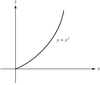
Chapter 2 covers the differential calculus of functions of one variable: limits, continu-ity, differentiablilcontinu-ity, L’Hospital’s rule, and Taylor’s theorem. The emphasis is on rigorous presentation of principles; no attempt is made to develop the properties of specific ele-mentary functions. Even though this may not be done rigorously in most contemporary calculus courses, I believe that the student’s time is better spent on principles rather than on reestablishing familiar formulas and relationships.

Chapter 3 is to devoted to the Riemann integral of functions of one variable. In Sec-tion 3.1 the integral is defined in the standard way in terms of Riemann sums. Upper and lower integrals are also defined there and used in Section 3.2 to study the existence of the integral. Section 3.3 is devoted to properties of the integral. Improper integrals are studied in Section 3.4. I believe that my treatment of improper integrals is more detailed than in most comparable textbooks. A more advanced look at the existence of the proper Riemann integral is given in Section 3.5, which concludes with Lebesgue’s existence criterion. This section can be omitted without compromising the student’s preparedness for subsequent sections.

Chapter 4 treats sequences and series. Sequences of constant are discussed in Sec-tion 4.1. I have chosen to make the concepts of limit inferior and limit superior parts of this development, mainly because this permits greater flexibility and generality, with little extra effort, in the study of infinite series. Section 4.2 provides a brief introduction to the way in which continuity and differentiability can be studied by means of sequences. Sections 4.3–4.5 treat infinite series of constant, sequences and infinite series of functions, and power series, again in greater detail than in most comparable textbooks. The instruc-tor who chooses not to cover these sections completely can omit the less standard topics without loss in subsequent sections.

Chapter 5 is devoted to real-valued functions of several variables. It begins with a dis-cussion of the toplogy ofRn_{in Section 5.1. Continuity and differentiability are discussed}

Chapter 6 covers the differential calculus of vector-valued functions of several variables. Section 6.1 reviews matrices, determinants, and linear transformations, which are integral parts of the differential calculus as presented here. In Section 6.2 the differential of a vector-valued function is defined as a linear transformation, and the chain rule is discussed in terms of composition of such functions. The inverse function theorem is the subject of Section 6.3, where the notion of branches of an inverse is introduced. In Section 6.4. the implicit function theorem is motivated by first considering linear transformations and then stated and proved in general.

Chapter 7 covers the integral calculus of real-valued functions of several variables. Mul-tiple integrals are defined in Section 7.1, first over rectangular parallelepipeds and then over more general sets. The discussion deals with the multiple integral of a function whose discontinuities form a set of Jordan content zero. Section 7.2 deals with the evaluation by iterated integrals. Section 7.3 begins with the definition of Jordan measurability, followed by a derivation of the rule for change of content under a linear transformation, an intuitive formulation of the rule for change of variables in multiple integrals, and finally a careful statement and proof of the rule. The proof is complicated, but this is unavoidable.

Chapter 8 deals with metric spaces. The concept and properties of a metric space are introduced in Section 8.1. Section 8.2 discusses compactness in a metric space, and Sec-tion 8.3 discusses continuous funcSec-tions on metric spaces.

Corrections–mathematical and typographical–are welcome and will be incorporated when received.

William F. Trench wtrench@trinity.edu Home: 659 Hopkinton Road

The Real Numbers

IN THIS CHAPTER we begin the study of the real number system. The concepts discussed here will be used throughout the book.

SECTION 1.1 deals with the axioms that define the real numbers, definitions based on them, and some basic properties that follow from them.

SECTION 1.2 emphasizes the principle of mathematical induction.

SECTION 1.3 introduces basic ideas of set theory in the context of sets of real num-bers. In this section we prove two fundamental theorems: the Heine–Borel and Bolzano– Weierstrass theorems.

1.1 THE REAL NUMBER SYSTEM

Having taken calculus, you know a lot about the real number system; however, you prob-ably do not know that all its properties follow from a few basic ones. Although we will not carry out the development of the real number system from these basic properties, it is useful to state them as a starting point for the study of real analysis and also to focus on one property, completeness, that is probably new to you.

Field Properties

The real number system (which we will often call simply thereals) is first of all a set fa; b; c; : : :_g on which the operations of addition and multiplication are defined so that every pair of real numbers has a unique sum and product, both real numbers, with the following properties.

(A)

(B)

(C)

(D)

(E)

The manipulative properties of the real numbers, such as the relations

.a_Cb/2_Da2_C2ab_Cb2;

.3a_C2b/.4c_C2d /_D12ac_C6ad_C8bc_C4bd;

. a/_D. 1/a; a. b/_D. a/b _D ab;

and

a bC

c

d D

ad_Cbc

bd .b; d ¤0/;

all follow from

(A)

(E)

A set on which two operations are defined so as to have properties

(A)

(E)

0_C0_D1_C1_D0; 1_C0_D0_C1_D1; (1.1.1)

and multiplication defined by

00_D01_D10_D0; 11_D1 (1.1.2)

(Exercise1.1.2).

The Order Relation

The real number system is ordered by the relation<, which has the following properties.

(F)

a_Db; a < b; or b < a:

(G)

(H)

A field with an order relation satisfying

(F)

(H)

We assume that you are familiar with other standard notation connected with the order relation: thus,a > bmeans thatb < a;a bmeans that eithera_D bora > b;a b means that eithera _D bora < b; theabsolute value of a, denoted byja_j, equals aif a0or aifa0. (Sometimes we callja_jthemagnitudeofa.)

Theorem 1.1.1 (The Triangle Inequality)

then

ja_Cb_{j j}a_{j C j}b_j: (1.1.3)

Proof

(a)

(b)

(c)

(d)

(c)

(d)

ja_Cb_{j D} (

ja_{j j}b_j ifja_{j j}b_j; jb_{j j}a_j if_jb_{j j}a_j:

The triangle inequality appears in various forms in many contexts. It is the most impor-tant inequality in mathematics. We will use it often.

Corollary 1.1.2

ja b_j ˇˇ_ja_{j j}b_jˇˇ (1.1.4)

and

ja_Cb_j ˇˇ_ja_{j j}b_jˇˇ: (1.1.5)

Proof

ja_{j j}a b_{j C j}b_j;

so

ja b_{j j}a_{j j}b_j: (1.1.6)

Interchangingaandbhere yields

jb a_{j j}b_{j j}a_j;

which is equivalent to

ja b_{j j}b_{j j}a_j; (1.1.7)

since_jb a_{j D j}a b_j. Since

ˇ

ˇ_ja_{j j}b_jˇˇ_D (

ja_{j j}b_j if _ja_j>_jb_j; jb_{j j}a_j if _jb_j>_ja_j;

(1.1.6) and (1.1.7) imply (1.1.4). Replacingbby bin (1.1.4) yields (1.1.5), since_j b_{j D}

jb_j.

Supremum of a Set

A setS of real numbers isbounded aboveif there is a real numberbsuch that x b whenever x ₂ S. In this case, bis anupper boundofS. Ifbis an upper bound ofS, then so is any larger number, because of property

(G)

With the real numbers associated in the usual way with the points on a line, these defini-tions can be interpreted geometrically as follows:bis an upper bound ofSif no point ofS is to the right ofb;ˇ_DsupSif no point ofS is to the right ofˇ, but there is at least one point ofSto the right of any number less thanˇ(Figure1.1.1).

(S = dark line segments)

β b

Figure 1.1.1

Example 1.1.1

This example shows that a supremum of a set may or may not be in the set, sinceS1 contains its supremum, butSdoes not.

Anonemptyset is a set that has at least one member. Theempty set, denoted by_;, is the set that has no members. Although it may seem foolish to speak of such a set, we will see that it is a useful idea.

The Completeness Axiom

It is one thing to define an object and another to show that there really is an object that satisfies the definition. (For example, does it make sense to define the smallest positive real number?) This observation is particularly appropriate in connection with the definition of the supremum of a set. For example, the empty set is bounded above by every real number, so it has no supremum. (Think about this.) More importantly, we will see in Example1.1.2 that properties

(A)

(H)

(I)

(I)

(A)

(I)

Theorem 1.1.3

(a)

Proof

(a)

(b)

(a)

(b)

(a)

(b)

Now we show that there cannot be more than one real number with properties

(a)

(b)

(b)

x0> ˇ2 .ˇ2 ˇ1/Dˇ1;

soˇ1 cannot have property

(a)

(a)

(b)

Some Notation

We will often define a setS by writingS _D˚xˇˇ , which means thatS consists of all xthat satisfy the conditions to the right of the vertical bar; thus, in Example1.1.1,

S _D˚xˇˇx < 0 (1.1.8)

and

S1D

˚

xˇˇxis a negative integer :

We will sometimes abbreviate “xis a member ofS” byx₂S, and “xis not a member of S” byx_…S. For example, ifSis defined by (1.1.8), then

1₂S but 0_…S:

The Archimedean Property

The property of the real numbers described in the next theorem is called theArchimedean property. Intuitively, it states that it is possible to exceed any positive number, no matter how large, by adding an arbitrary positive number, no matter how small, to itself sufficiently many times.

Theorem 1.1.4 (

Archimedean

Property)

Proof

S _D˚xˇˇx _Dn; nis an integer : Therefore,S has a supremumˇ, by property

(I)

Sincen_C1is an integer whenevernis, (1.1.9) implies that

.n_C1/ˇ

and therefore

nˇ

for all integersn. Hence,ˇ is an upper bound ofS. Sinceˇ < ˇ, this contradicts the definition ofˇ.

Density of the Rationals and Irrationals

Definition 1.1.5

Theorem 1.1.6

Proof

qa < pqa_C1: Since1 < q.b a/, this implies that

qa < p < qa_Cq.b a/_Dqb; soqa < p < qb. Therefore,a < p=q < b.

Example 1.1.2

S _D˚rˇˇris rational andr2< 2 :

Ifr ₂S, thenr <p2. Theorem1.1.6implies that if > 0there is a rational numberr0 such thatp2 < r0<

p

2, so Theorem1.1.3implies thatp2_DsupS. However,p2is irrational; that is, it cannot be written as the ratio of integers (Exercise1.1.3). Therefore, ifr1is any rational upper bound ofS, then

p

2 < r1. By Theorem1.1.6, there is a rational numberr2such that

p

2 < r2< r1. Sincer2is also a rational upper bound ofS, this shows thatShas no rational supremum.

Since the rational numbers have properties

(A)

(H)

(I)

(I)

(A)

(H)

Theorem 1.1.7

Proof

a < r1< r2< b: (1.1.10)

Let

t _Dr1C

1 p

2.r2 r1/:

Thentis irrational (why?) andr1 < t < r2, soa < t < b, from (1.1.10).

Infimum of a Set

A setS of real numbers isbounded below if there is a real numberasuch that x a wheneverx ₂ S. In this case,ais alower boundofS. Ifais a lower bound ofS, so is any smaller number, because of property

(G)

˛_DinfS:

Geometrically, this means that there are no points ofSto the left of˛, but there is at least one point ofSto the left of any number greater than˛.

Theorem 1.1.8

(a)

(b)

Proof

A setS isboundedif there are numbersaandbsuch thatax bfor allxinS. A bounded nonempty set has a unique supremum and a unique infimum, and

infS supS (1.1.11)

(Exercise1.1.7).

The Extended Real Number System

A nonempty setS of real numbers isunbounded above if it has no upper bound, or un-bounded belowif it has no lower bound. It is convenient to adjoin to the real number system two fictitious points,C1(which we usually write more simply as 1) and 1, and to define the order relationships between them and any real numberxby

1< x <₁: (1.1.12)

We call₁and ₁points at infinity. IfSis a nonempty set of reals, we write

supS_{D 1} (1.1.13)

to indicate thatSis unbounded above, and

infS _{D 1} (1.1.14)

Example 1.1.3

S_D˚xˇˇx < 2 ; then supS_D2and infS_{D 1}. If

S _D˚xˇˇx 2 ;

then supS _{D 1} and infS _D 2. IfS is the set of all integers, then supS _{D 1}and infS _{D 1}.

The real number system with1and 1adjoined is called theextended real number system, or simply theextended reals. A member of the extended reals differing from 1 and1isfinite; that is, an ordinary real number is finite. However, the word “finite” in “finite real number” is redundant and used only for emphasis, since we would never refer to₁or ₁as real numbers.

The arithmetic relationships among1, 1, and the real numbers are defined as follows.

(a)

a_{C 1 D 1 C}a_{D 1};

a _{1 D 1 C}a_{D 1};

a

1 D

a 1 D0:

(b)

a_{1 D 1}a _{D 1};

a . ₁/_D. ₁/ a_{D 1}:

(c)

a_{1 D 1}a _{D 1};

a . ₁/_D. ₁/ a_{D 1}:

We also define

1 C 1 D 11 D. ₁/. ₁/_{D 1} and

1 1 D 1. ₁/_D. ₁/_{1 D 1}: Finally, we define

j1j D j 1j D 1:

It is not useful to define1 1,0 ₁,1=₁, and0=0. They are calledindeterminate forms, and left undefined. You probably studied indeterminate forms in calculus; we will look at them more carefully in Section 2.4.

1.1 Exercises

1.

(a)

(b)

(c)

(d)

2.

(F)

(G)

(H)

3.

4.

5.

(a)

(b)

(c)

(d)

(e)

(f )

6.

(I)

7.

(a)

infS supS .A/

for any nonempty setS of real numbers, and give necessary and sufficient conditions for equality.

(b)

8.

9.

(A)

(H)

Sbe the set of real numbers that are not upper bounds ofU:

10.

S_CT _D˚s_Ctˇˇs₂S; t ₂T :

(a)

sup.S_CT /_DsupS_CsupT .A/

ifS andT are bounded above and

inf.S_CT /_DinfS_CinfT .B/ ifS andT are bounded below.

(b)

11.

(a)

sup.S T /_DsupS infT .A/

and

inf.S T /_DinfS supT: .B/

(b)

12.

1.2 MATHEMATICAL INDUCTION

If a flight of stairs is designed so that falling off any step inevitably leads to falling off the next, then falling off the first step is a sure way to end up at the bottom. Crudely expressed, this is the essence of theprinciple of mathematical induction: If the truth of a statement depending on a given integer nimplies the truth of the corresponding statement with n replaced byn_C1, then the statement is true for all positive integersnif it is true forn_D1. Although you have probably studied this principle before, it is so important that it merits careful review here.

Peano’s Postulates and Induction

The rigorous construction of the real number system starts with a setN_{of undefined}

(A)

(B)

(C)

(D)

(E)

itself.

These axioms are known as Peano’s postulates. The real numbers can be constructed from the natural numbers by definitions and arguments based on them. This is a formidable task that we will not undertake. We mention it to show how little you need to start with to construct the reals and, more important, to draw attention to postulate

(E)

It can be shown that the positive integers form a subset of the reals that satisfies Peano’s postulates (withn_D1andn0_{DnC1), and it is customary to regard the positive integers}

and the natural numbers as identical. From this point of view, the principle of mathematical induction is basically a restatement of postulate

(E)

Theorem 1.2.1 (Principle of Mathematical Induction)

Pn;. . . be propositions;one for each positive integer;such that

(a)

(b)

Proof

M_D˚_nˇˇ_n2N_{andPnis true :}

From

(a)

(b)

postulate

(E)

Example 1.2.1

1_C2_{C C}n_D n.nC1/

2 : (1.2.1)

ThenP1 is the proposition that1 D 1, which is certainly true. IfPnis true, then adding

n_C1to both sides of (1.2.1) yields

.1_C2_{C C}n/_C.n_C1/_D n.nC1/

2 C.nC1/

D.n_C1/n 2 C1

D .nC1/.nC2/

2 ;

or

1_C2_{C C}.n_C1/_D .nC1/.nC2/

which isPnC1, since it has the form of (1.2.1), withnreplaced bynC1. Hence,Pnimplies

PnC1, so (1.2.1) is true for alln, by Theorem1.2.1.

A proof based on Theorem 1.2.1 is aninduction proof, or proof by induction. The assumption thatPnis true is theinduction assumption. (Theorem1.2.3permits a kind of induction proof in which the induction assumption takes a different form.)

Induction, by definition, can be used only to verify results conjectured by other means. Thus, in Example1.2.1we did not use induction tofindthe sum

snD1C2C CnI (1.2.2)

rather, weverifiedthat

snD

n.n_C1/

2 : (1.2.3)

How you guess what to prove by induction depends on the problem and your approach to it. For example, (1.2.3) might be conjectured after observing that

s1D1D

12

2 ; s2D3D 23

2 ; s3D6D 43

2 :

However, this requires sufficient insight to recognize that these results are of the form (1.2.3) forn _D 1,2, and3. Although it is easy to prove (1.2.3) by induction once it has been conjectured, induction is not the most efficient way to findsn, which can be obtained quickly by rewriting (1.2.2) as

snDnC.n 1/C C1 and adding this to (1.2.2) to obtain

2snDŒnC1CŒ.n 1/C2C CŒ1Cn:

There are nbracketed expressions on the right, and the terms in each add up to n_C1; hence,

2snDn.nC1/; which yields (1.2.3).

The next two examples deal with problems for which induction is a natural and efficient method of solution.

Example 1.2.2

anC1 D

1

n_C1an; n1 (1.2.4)

(we say thatanis definedinductively), and suppose that we wish to find an explicit formula foran. By consideringnD1,2, and3, we find that

a1D

1

1; a2D 1

and therefore we conjecture that

anD

1

nŠ: (1.2.5)

This is given forn_D1. If we assume it is true for somen, substituting it into (1.2.4) yields

anC1D

1 n_C1

1 nŠ D

1 .n_C1/Š;

which is (1.2.5) withn replaced byn_C1. Therefore, (1.2.5) is true for every positive integern, by Theorem1.2.1.

Example 1.2.3

jxnC1 xnj rjxn xn 1j; n1; (1.2.6) whereris a fixed positive number. By considering (1.2.6) forn_D1,2, and3, we find that

jx2 x1j rjx1 x0j;

jx3 x2j rjx2 x1j r2jx1 x0j;

jx4 x3j rjx3 x2j r3jx1 x0j: Therefore, we conjecture that

jxn xn 1j rn 1jx1 x0j if n1: (1.2.7) This is trivial forn_D1. If it is true for somen, then (1.2.6) and (1.2.7) imply that

jxnC1 xnj r .rn 1jx1 x0j/; so jxnC1 xnj rnjx1 x0j;

which is proposition (1.2.7) with nreplaced byn_C1. Hence, (1.2.7) is true for every positive integern, by Theorem1.2.1.

The major effort in an induction proof (afterP1,P2, . . . ,Pn, . . . have been formulated) is usually directed toward showing thatPnimpliesPnC1. However, it is important to verify

P1, sincePnmay implyPnC1even if some or all of the propositionsP1,P2, . . . , Pn, . . . are false.

Example 1.2.4

2n_C1_D.2n 1/_C2:

Theorem 1.2.2

(a)

(b)

Proof

(a)

(b)

Example 1.2.5

3n_C16 > 0: IfPnis true, then so isPnC1, since

3.n_C1/_C16_D3n_C3_C16

D.3n_C16/_C3 > 0_C3(by the induction assumption) > 0:

The smallest n0 for whichPn0 is true isn0 D 5. Hence, Pn is true forn 5, by Theorem1.2.2.

Example 1.2.6

nŠ 3n> 0: IfPnis true, then

.n_C1/Š 3nC1_DnŠ.n_C1/ 3nC1

> 3n.n_C1/ 3nC1 (by the induction assumption) D3n.n 2/:

Therefore, PnimpliesPnC1ifn > 2. By trial and error,n0 D 7is the smallest integer such thatPn0 is true; hence,Pnis true forn7, by Theorem1.2.2.

The next theorem is a useful consequence of the principle of mathematical induction.

Theorem 1.2.3

(a)

Proof

(a)

(b)

Example 1.2.7

4_D22; 6_D23; 8_D222; 9_D33; 10_D25:

These observations suggest that each integern 2is a prime or a product of primes. Let this proposition bePn. Then P2 is true, but neither Theorem 1.2.1nor Theorem 1.2.2 apply, sincePndoes not implyPnC1 in any obvious way. (For example, it is not evident from24_D2 2 2 3that 25 is a product of primes.) However, Theorem1.2.3yields the stated result, as follows. Suppose thatn 2andP2, . . . ,Pnare true. EithernC1is a prime or

n_C1_Dr s; (1.2.8)

whererandsare integers and1 < r,s < n, soPrandPsare true by assumption. Hence,r andsare primes or products of primes and (1.2.8) implies thatn_C1is a product of primes. We have now provedPnC1(thatnC1is a prime or a product of primes). Therefore,Pnis true for alln2, by Theorem1.2.3.

1.2 Exercises

Prove the assertions in Exercises1.2.1–1.2.6by induction.

1.

2.

6 :

3.

2 _1/

3 :

4.

ja1Ca2C Canj ja1j C ja2j C C janj:

5.

.1_Ca1/.1Ca2/ .1Can/1Ca1Ca2C Can:

6.

7.

8.

xnC1 D

1 2

R xnC

xn

; n0:

Prove: Forn1,xn> xnC1>pRand

xn

p

R 1

2n

.x0

p R/2 x0

:

9.

(a)

an

.n_C1/.2n_C1/

(b)

3an

.2n_C2/.2n_C3/

(c)

2n_C1

n_C1 an

(d)

1_C 1

n n

an

10.

anDnŠ

(a)

(b)

11.

1_C2_{C C}n_D .nC2/.n 1/

2 :

(a)

(b)

12.

1 nŠ >

8n

.2n/Š‹ Prove your answer by induction.

13.

(a)

(b)

(a)

(c)

(a)

(b)

n_Dp1 pr and nDq1q2 qs;

wherep1, . . . ,pr,q1, . . . ,qsare positive primes, thenr Dsandfq1; : : : ; qrg is a permutation of_fp1; : : : ; prg.

15.

anC1DanC6an 1; n2: Show by induction thatanD3n . 2/nifn1.

16.

anC1D9an 23an 1C15an 2; n3: Show by induction thatanD3n 1 5n 1C2,n1.

17.

FnC1DFnCFn 1; n2: Prove by induction that

FnD

.1_Cp5/n _.1 p_5/n

2np₅ ; n1:

18.

0

yn.1 y/rdy_D nŠ

.r_C1/.r_C2/ .r_Cn_C1/ ifnis a nonnegative integer andr > 1.

19.

m !

is the coefficient oftmin the expansion of.1_Ct /n; that is, .1_Ct /n_D

n

X

mD0

n m !

tm: From this definition it follows immediately that

n 0 !

D n

n !

D1; n0:

For convenience we define

n 1

!

D n

n_C1 !

(a)

n_C1 m

! D _mn

!

C _mn ₁ !

; 0mn;

and use this to show by induction onnthat

n m !

D nŠ

mŠ.n m/Š; 0mn:

(b)

n

X

mD0

. 1/m n m !

D0 and n

X

mD0

n m !

D2n:

(c)

.x_Cy/n_D

n

X

mD0

n m !

xmyn m:

(This is thebinomial theorem.)

20.

21.

fn.x1; x2; : : : ; xn/Dfn 1.x1; x2; : : : ; xn 1/C2n 2xnC

jfn 1.x1; x2; : : : ; xn 1/ 2n 2xnj and

gn.x1; x2; : : : ; xn/Dgn 1.x1; x2; : : : ; xn 1/C2n 2xn

jgn 1.x1; x2; : : : ; xn 1/ 2n 2xnj: Find explicit formulas forfn.x1; x2; : : : ; xn/andgn.x1; x2; : : : ; xn/.

22.

sinx_Csin3x_{C C}sin.2n 1/x_D 1 cos2nx

2sinx ; n1:

HINT:You will need trigonometric identities that you can derive from the identities

cos.A B/_DcosAcosB_CsinAsinB; cos.A_CB/_DcosAcosB sinAsinB:

23.

Q.`1; `2; : : : ; `n/D n

X

iD1

.ai b`i/ 2_:

Show that

Q.`1; `2; : : : ; `n/Q.1; 2; : : : ; n/:

1.3 THE REAL LINE

One of our objectives is to develop rigorously the concepts of limit, continuity, differen-tiability, and integrability, which you have seen in calculus. To do this requires a better understanding of the real numbers than is provided in calculus. The purpose of this section is to develop this understanding. Since the utility of the concepts introduced here will not become apparent until we are well into the study of limits and continuity, you should re-serve judgment on their value until they are applied. As this occurs, you should reread the applicable parts of this section. This applies especially to the concept of an open covering and to the Heine–Borel and Bolzano–Weierstrass theorems, which will seem mysterious at first.

We assume that you are familiar with the geometric interpretation of the real numbers as points on a line. We will not prove that this interpretation is legitimate, for two reasons: (1) the proof requires an excursion into the foundations of Euclidean geometry, which is not the purpose of this book; (2) although we will use geometric terminology and intuition in discussing the reals, we will base all proofs on properties

(A)

(I)

Henceforth, we will use the termsreal number systemandreal linesynonymously and denote both by the symbolR_{; also, we will often refer to a real number as a}point(on the real line).

Some Set Theory

In this section we are interested in sets of points on the real line; however, we will consider other kinds of sets in subsequent sections. The following definition applies to arbitrary sets, with the understanding that the members of all sets under consideration in any given context come from a specific collection of elements, called theuniversal set. In this section the universal set is the real numbers.

Definition 1.3.1

(a)

(b)

(d)

(e)

(f )

(b)

(g)

(c)

(d)

(h)

T S

S T

(a)

S∪ T =shaded region (b)

(c) (d)

S∩ T =shaded region S∩ T = ∅ T

S

T S

T S

Figure 1.3.1

Example 1.3.1

S_D˚xˇˇ0 < x < 1 ; T _D˚xˇˇ0 < x < 1andxis rational ;

and

U _D˚xˇˇ0 < x < 1andxis irrational :

ThenS T andSU, and the inclusion is strict in both cases. The unions of pairs of these sets are

S_[T _DS; S_[U _DS; and T _[U _DS;

and their intersections are

Also,

S U _DT and S T _DU:

Every setScontains the empty set;, for to say that;is not contained inSis to say that some member of;is not inS, which is absurd since;has no members. IfS is any set, then

.Sc/c _DS and S_\Sc _{D ;}: IfSis a set of real numbers, thenS_[Sc _DR_.

The definitions of union and intersection have generalizations: IfF _{is an arbitrary}

col-lection of sets, then[˚SˇˇS ₂F _{is the set of all elements that are members of at least}

one of the sets inF_{, and\}˚_Sˇˇ_{S 2}F _{is the set of all elements that are members of every}

set inF_{. The union and intersection of finitely many setsS1, . . . ,Snare also written as}

Sn

kD1SkandTnkD1Sk. The union and intersection of an infinite sequencefSkg1_kD1of sets are written asS1kD1SkandT1kD1Sk.

Example 1.3.2

SD

˚

xˇˇ < x1_C ; 0 < 1=2;

then [ ˚

S

ˇ

ˇS2F D

˚

xˇˇ0 < x3=2 and \ ˚S

ˇ

ˇS2F D

˚

xˇˇ1=2 < x1 :

Example 1.3.3

Open and Closed Sets

Ifaandbare in the extended reals anda < b, then theopen interval.a; b/is defined by

.a; b/_D˚xˇˇa < x < b :

The open intervals.a;₁/and. ₁; b/aresemi-infiniteifaandbare finite, and. ₁;₁/ is the entire real line.

( )

x 0 + x

0 − x0

x₀ = interior point of S S = four line segments

Figure 1.3.2

The idea of neighborhood is fundamental and occurs in many other contexts, some of which we will see later in this book. Whatever the context, the idea is the same: some defi-nition of “closeness” is given (for example, two real numbers are “close” if their difference is “small”), and a neighborhood of a pointx0is a set that contains all points sufficiently close tox0.

Example 1.3.4

min_fx0 a; b x0g, then

.x0 ; x0C/.a; b/:

The entire lineR_D . ₁;₁/is open, and therefore;._D Rc/is closed. However, ;is also open, for to deny this is to say that_;contains a point that is not an interior point, which is absurd because_;contains no points. Since_;is open,R._{D ;}c/is closed. Thus,

R and_;are both open and closed. They are the only subsets of R with this property (Exercise1.3.18).

Adeleted neighborhoodof a pointx0is a set that contains every point of some neigh-borhood ofx0except forx0itself. For example,

S _D˚xˇˇ0 <_jx x0j<

is a deleted neighborhood ofx0. We also say that it is adeleted-neighborhoodofx0.

Theorem 1.3.3

(a)

(b)

These statements apply to arbitrary collections, finite or infinite, of open and closed sets:

Proof (a)

S _{D [}˚GˇˇG₂G :

Ifx0 2 S, thenx0 2 G0 for someG0 inG, and sinceG0 is open, it contains some -neighborhood ofx0. SinceG0S, this-neighborhood is inS, which is consequently a neighborhood ofx0. Thus,S is a neighborhood of each of its points, and therefore open, by definition.

(b)

[˚FcˇˇF ₂F _{(Exercise1.3.7) and, since eachF}c_{is open,T}c_{is open, from}

(a)

Example 1.3.5

Œa; b_D˚xˇˇaxb

is closed, since its complement is the union of the open sets. ₁; a/and.b;₁/. We say thatŒa; bis aclosed interval. The set

Œa; b/_D˚xˇˇax < b

is ahalf-closedorhalf-open intervalif ₁< a < b <₁, as is

.a; b_D˚xˇˇa < xb _I

however, neither of these sets is open or closed. (Why not?)Semi-infinite closed intervals are sets of the form

Œa;₁/_D˚xˇˇax and . ₁; a_D˚xˇˇxa ;

wherea is finite. They are closed sets, since their complements are the open intervals . ₁; a/and.a;₁/, respectively.

Example1.3.4shows that a set may be both open and closed, and Example1.3.5shows that a set may be neither. Thus, open and closed are not opposites in this context, as they are in everyday speech.

Example 1.3.6

R_{is the union of open intervals.) From Theorem1.3.3and Example1.3.5, the intersection}

of any collection of closed intervals is closed.

It can be shown that the intersection of finitely many open sets is open, and that the union of finitely many closed sets is closed. However, the intersection of infinitely many open sets need not be open, and the union of infinitely many closed sets need not be closed (Exercises1.3.8and1.3.9).

Definition 1.3.4

(a)

(b)

(c)

(d)

(a)

(b)

(c)

(d)

Example 1.3.8

InD

1 2n_C1;

1 2n

and S _D

1

[

nD1

In:

Then

(a)

(b)

(c)

(d)

. ₁; 0/_[ " ₁

[

nD1

1 2n_C2;

1 2n_C1

# [

1 2;1

:

Example 1.3.9

Since every interval also contains an irrational number (Theorem1.1.7), every real number is a boundary point ofS; thus@S _DR_{. The interior and exterior ofSare both empty, and}

Shas no isolated points.Sis neither open nor closed.

The next theorem says thatSis closed if and only ifS _DS(Exercise1.3.14).

Theorem 1.3.5

Proof

Theorem1.3.5is usually stated as follows.

Corollary 1.3.6

Open Coverings

A collectionH _{of open sets is an}open coveringof a setSif every point inSis contained in a setHbelonging toH_{; that is, if}S _[˚HˇˇH ₂H _.

Example 1.3.10

S1DŒ0; 1; S2D f1; 2; : : : ; n; : : :g;

S3D

1;1

2; : : : ; 1 n; : : :

; and S4D.0; 1/

are covered by the families of open intervals

H_1D

x 1

N; xC 1 N

ˇˇ_ˇ

ˇ0 < x < 1

; (N _Dpositive integer),

H_2D

n 1

4; nC 1 4

ˇˇ_ˇ

ˇnD1; 2; : : :

;

H_3D

( 1 n_C 1₂;

1 n 1₂

! ˇ_ˇ ˇ

ˇnD1; 2; : : : )

;

and

H_{4D f}.0; /_j0 < < 1_g; respectively.

Theorem 1.3.7 (

Heine

–

Borel

Theorem)

Proof

St DS\Œ˛; t  for t ˛; and let

F _D˚tˇˇ˛t ˇand finitely many sets fromH_{coverSt :}

SinceSˇ DS, the theorem will be proved if we can show thatˇ2F. To do this, we use the completeness of the reals.

Since˛₂S,S˛is the singleton setf˛g, which is contained in some open setH˛from H _becauseH _{coversS; therefore,˛2F. SinceF is nonempty and bounded above byˇ,}

CASE1. Suppose that < ˇand ₆₂S. Then, sinceSis closed,is not a limit point ofS(Theorem1.3.5). Consequently, there is an > 0such that

Œ ; _C_\S_{D ;};

soS _D SC. However, the definition of implies thatS has a finite subcovering fromH_{, whileSCdoes not. This is a contradiction.}

CASE 2. Suppose that < ˇand ₂ S. Then there is an open setH inH that containsand, along with, an intervalŒ ; _Cfor some positive. SinceS has a finite coveringfH1; : : : ; Hngof sets fromH, it follows thatSChas the finite covering

fH1; : : : ; Hn; Hg. This contradicts the definition of.

Now we know that _Dˇ, which is inS. Therefore, there is an open setHˇinH that containsˇand along withˇ, an interval of the formŒˇ ; ˇ_C, for some positive. SinceSˇ is covered by a finite collection of setsfH1; : : : ; Hkg,Sˇ is covered by the finite collectionfH1; : : : ; Hk; Hˇg. SinceSˇ DS, we are finished.

Henceforth, we will say that a closed and bounded set is compact. The Heine–Borel theorem says that any open covering of a compact setS contains a finite collection that also covers S. This theorem and its converse (Exercise1.3.21) show that we could just as well define a setSof reals to be compact if it has the Heine–Borel property; that is, if every open covering ofScontains a finite subcovering. The same is true ofRn_{, which we}

study in Section 5.1. This definition generalizes to more abstract spaces (calledtopological spaces) for which the concept of boundedness need not be defined.

Example 1.3.11

k2N 1/coverS1.

The Heine–Borel theorem does not apply to the other sets in Example1.3.10since they are not compact:S2is unbounded andS3andS4are not closed, since they do not contain all their limit points (Corollary1.3.6). The conclusion of the Heine–Borel theorem does not hold for these sets and the open coverings that we have given for them. Each point in S2 is contained in exactly one set fromH2, so removing even one of these sets leaves a point ofS2uncovered. IfHe3is any finite collection of sets fromH3, then

1 n 62 [

˚

HˇˇH ₂He₃

fornsufficiently large. Any finite collection_f.0; 1/; : : : ; .0; n/gfromH4covers only the interval.0; max/, where

maxDmaxf1; : : : ; ng< 1:

The Bolzano–Weierstrass Theorem

Theorem 1.3.8 (

Bolzano

–

Weierstrass

Theorem)

Proof

H _D˚_Nxˇˇ_x2S

is an open covering forS. SinceSis also bounded, Theorem1.3.7implies thatS can be covered by a finite collection of sets fromH_{, sayNx1, . . . ,Nxn. Since these sets contain}

onlyx1, . . . ,xnfromS, it follows thatSD fx1; : : : ; xng.

1.3 Exercises

1.

(a)

(b)

(c)

(d)

2.

(a)

1

[

kD1

Sk

(b)

1

\

kD1

Sk

(c)

1

[

kD1

S_kc

(d)

1

\

kD1

S_kc

3.

4.

(a)

₁

2; 1

(b)

₁

2; 3 2

(c)

(d)

5.

(a)

(b)

(c)

(d)

6.

7.

I _{D \}˚FˇˇF ₂F _{and U D [}˚_Fˇˇ_{F 2}F _:

Prove that

(a)

(b)

(b)

9.

(a)

(b)

10.

(a)

(b)

11.

(a)

(b)

(c)

(d)

12.

13.

14.

(a)

(b)

15.

16.

(a)

(b)

17.

18.

19.

(a)

(b)

(c)

(d)

(e)

20.

(a)

(b)

(c)

(d)

(e)

(f )

(g)

21.

has an open coveringHe _{comprised of finitely many open sets from}H_{. Show that}

Sis compact.

22.

(a)

(b)

(a)

23.

(a)

(b)

24.

(a)

(b)

(c)

(d)

Differential Calculus of

Functions of One Variable

IN THIS CHAPTER we study the differential calculus of functions of one variable. SECTION 2.1 introduces the concept of function and discusses arithmetic operations on functions, limits, one-sided limits, limits at˙1, and monotonic functions.

SECTION 2.2 defines continuity and discusses removable discontinuities, composite func-tions, bounded funcfunc-tions, the intermediate value theorem, uniform continuity, and addi-tional properties of monotonic functions.

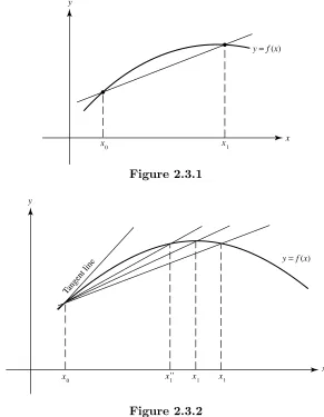
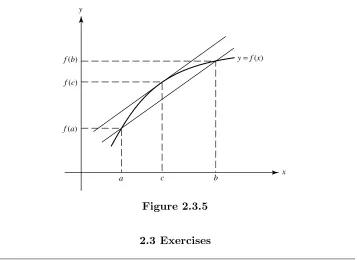
SECTION 2.3 introduces the derivative and its geometric interpretation. Topics covered in-clude the interchange of differentiation and arithmetic operations, the chain rule, one-sided derivatives, extreme values of a differentiable function, Rolle’s theorem, the intermediate value theorem for derivatives, and the mean value theorem and its consequences.

SECTION 2.4 presents a comprehensive discussion of L’Hospital’s rule.

SECTION 2.5 discusses the approximation of a functionf by the Taylor polynomials of f and applies this result to locating local extrema off. The section concludes with the extended mean value theorem, which implies Taylor’s theorem.

2.1 FUNCTIONS AND LIMITS

In this section we study limits of real-valued functions of a real variable. You studied limits in calculus. However, we will look more carefully at the definition of limit and prove theorems usually not proved in calculus.

A rulef that assigns to each member of a nonempty setDa unique member of a setY is afunction fromDtoY. We write the relationship between a memberxofDand the memberyofY thatf assigns toxas

y_Df .x/:

The setDis thedomainoff, denoted byDf. The members ofY are the possiblevalues off. Ify02Y and there is anx0inDsuch thatf .x0/Dy0then we say thatf attains

orassumesthe valuey0. T