Active Calculus Multivariable

(1)

MULTIVARIABLE

2017 Edition

Steven Schlicker

(2)

Active Calculus - Multivariable

2017 edition

Steve Schlicker, Lead Author and Editor Department of Mathematics Grand Valley State University

[email protected]

http://faculty.gvsu.edu/schlicks/

David Austin, Contributing Author

http://merganser.math.gvsu.edu/david/

Matt Boelkins, Contributing Author

http://faculty.gvsu.edu/boelkinm/

(3)

(4)

Preface

A free and open-source calculus

As we have noted in the single-variable edition ofActive Calculus, several fundamental ideas in calculus are more than 2000 years old, and calculus as a formal subdiscipline of mathematics was first introduced and developed in the late 1600s. Mathematicians agree that the subject has been understood – rigorously and by experts – since the mid 1800s. The discipline is one of our great human intellectual achievements.

While each author of a calculus textbook certainly offers their own creative perspective on the subject, it is hardly the case that many of the ideas the author presents are new. Indeed, the mathematics community broadly agrees on what the main ideas of calculus are, as well as their justification and their importance; the core parts of nearly all calculus textbooks are very similar. As such, it is our opinion that in the 21st century – an age where the internet permits seamless and immediate transmission of information – no one should be required to purchase a calculus text to read, to use for a class, or to find a coherent collection of problems to solve. Calculus belongs to humankind, not any individual author or publishing company. Thus, a main purpose of this work is to present a new multivariable calculus text that isfree. In addition, instructors who are looking for a multivariable calculus text should have the opportunity to download the source files and make modifications that they see fit; thus this text isopen-source.

Any professor or student may use an electronic version of the text for no charge. A .pdf copy of the text may be obtained by download from theActive Calculus home page, or directly from

http://gvsu.edu/s/Wb.

Because the text is open-source, any instructor may acquire the full set of source files, by request via email to Steve Schlicker.

This work is licensed under the Creative Commons Attribution-NonCommercial-ShareAlike 3.0 Unported License. The graphic

(7)

that appears throughout the text shows that the work is licensed with the Creative Commons, that the work may be used for free by any party so long as attribution is given to the author(s), that the work and its derivatives are used in the spirit of “share and share alike,” and that no party may sell this work or any of its derivatives for profit. Full details may be found by visiting

http://creativecommons.org/licenses/by-nc-sa/3.0/

or sending a letter to Creative Commons, 444 Castro Street, Suite 900, Mountain View, California, 94041, USA.

Active Calculus - Multivariable: our goals

InActive Calculus - Multivariable, we endeavor to actively engage students in learning the subject through an activity-driven approach in which the vast majority of the examples are completed by students. Where many texts present a general theory of calculus followed by substantial collec-tions of worked examples, we instead pose problems or situacollec-tions, consider possibilities, and then ask students to investigate and explore. Following key activities or examples, the presentation normally includes some overall perspective and a brief synopsis of general trends or properties, followed by formal statements of rules or theorems. While we often offer plausibility arguments for such results, rarely do we include formal proofs. It is not the intent of this text for the instructor or author todemonstrateto students that the ideas of calculus are coherent and true, but rather for students to encounterthese ideas in a supportive, leading manner that enables them to begin to understand for themselves why calculus is both coherent and true.

This approach is consistent with the following goals:

• To have students engage in an active, inquiry-driven approach, where learners strive to con-struct solutions and approaches to ideas on their own, with appropriate support through questions posed, hints, and guidance from the instructor and text.

• To build in students intuition for why the main ideas in multivariable calculus are natural and true. We strive to accomplish this by using specific cases to highlight the ideas for the general situation using contexts that are common and familiar.

• To challenge students to acquire deep, personal understanding of multivariable calculus through reading the text and completing preview activities on their own, through working on activities in small groups in class, and through doing substantial exercises outside of class time.

(8)

vii

Features of the Text

Similar to the presentation of the single-variableActive Calculus, instructors and students alike will find several consistent features in the presentation, including:

• Motivating Questions. At the start of each section, we listmotivating questionsthat provide motivation for why the following material is of interest to us. One goal of each section is to answer each of the motivating questions.

• Preview Activities. Each section of the text begins with a short introduction, followed by apreview activity. This brief reading and the preview activity are designed to foreshadow the upcoming ideas in the remainder of the section; both the reading and preview activity are intended to be accessible to studentsin advanceof class, and indeed to be completed by students before a day on which a particular section is to be considered.

• Activities. Every section in the text contains several activities. These are designed to en-gage students in an inquiry-based style that encourages them to construct solutions to key examples on their own, working either individually or in small groups.

• Exercises. There are dozens of calculus texts with (collectively) tens of thousands of exer-cises. Rather than repeat standard and routine exercises in this text, we recommend the use of WeBWorK with its access to the National Problem Library and its many multivariable calculus problems. In this text, there are a small number of challenging exercises in each sec-tion. Almost every such exercise has multiple parts, requires the student to connect several key ideas, and expects that the student will do at least a modest amount of writing to answer the questions and explain their findings. For instructors interested in a more conventional source of exercises, consider the freely available text by Gilbert Strang of MIT, available in .pdf format from the MIT open courseware site viahttp://gvsu.edu/s/bh.

• Graphics. As much as possible, we strive to demonstrate key fundamental ideas visually, and to encourage students to do the same. Throughout the text, we use full-color graphics to exemplify and magnify key ideas, and to use this graphical perspective alongside both numerical and algebraic representations of calculus. The figures and the software to generate them have been created by David Austin.

• Links to Java Applets. Many of the ideas of multivariable calculus are best understood dynamically, and there are a number of applets referenced in the text that can be used by instructors and students to assist in the investigations and demonstrations. The use of these freely available applets is in accord with our philosophy that no one should be required to purchase materials to learn calculus. We are indebted to everyone who allows their expertise to be openly shared.

(9)

How to Use this Text

This text may be used as a stand-alone textbook for a standard multivariable calculus course or as a supplement to a more traditional text.

Electronically

Because students and instructors alike have access to the book in .pdf format, there are several advantages to the text over a traditional print text. One is that the text may be projected on a screen in the classroom (or even better, on a whiteboard) and the instructor may reference ideas in the text directly, add comments or notation or features to graphs, and indeed write right on the text itself. Students can do likewise, choosing to print only whatever portions of the text are needed for them. In addition, the electronic version of the text includes live html links to java applets, so student and instructor alike may follow those links to additional resources that lie outside the text itself. Finally, students can have access to a copy of the text anywhere they have an internet-enabled device.

Activities Workbook

Each section of the text has a preview activity and at least three in-class activities embedded in the discussion. As it is the expectation that students will complete all of these activities, it is ideal for them to have room to work on them adjacent to the problem statements themselves. As a separate document, we have compiled a workbook of activities that includes only the individual activity prompts, along with space provided for students to write their responses. This workbook is the one printing expense that students will almost certainly have to undertake, and is available upon request to the authors.

There are also options in the source files for compiling the activities workbook with hints for each activity, or even full solutions. These options can be engaged at the instructor’s discretion.

Community of Users

(10)

ix

Acknowledgments

This text is an extension of the single variableActive Calculusby Matt Boelkins. The initial drafts of this multivariable edition were written by Steve Schlicker; editing and revisions were made by David Austin and Matt Boelkins. David Austin is responsible for the beautiful full-color .eps graphics in the text. Many of our colleagues at GVSU have shared their ideas and resources, which undoubtedly had a significant influence on the product. We thank them for all of their support.

In advance, we also thank our colleagues throughout the mathematical community who will read, edit, and use this book, and hence contribute to its improvement through ongoing discus-sion. The following people have used early drafts of this text and have generously offered sugges-tions that have improved the text.

Jon Barker and students St. Ignatius High School, Cleveland, OH Brian Drake Grand Valley State University

Brian Gleason Nevada State College

Mitch Keller Washington & Lee University

In addition, we offer thanks to Lars Jensen for giving us permission to use his photograph of the Lake of the Clouds in the Porcupine Mountains State Park in Michigan’s upper peninsula for our cover. A contour plot of a portion of the Porcupine Mountains State Park is the focus of an activity in Section9.1.

The authors take responsibility for all errors or inconsistencies in the text, and welcome reader and user feedback to correct them, along with other suggestions to improve the text.

(11)

(12)

Chapter 9

Multivariable and Vector Functions

9.1

Functions of Several Variables and Three Dimensional Space

Motivating Questions

In this section, we strive to understand the ideas generated by the following important questions:

• What is a function of several variables? What do we mean by the domain of a function of several variables?

• How do we find the distance between two points inR3? What is the equation of a sphere inR3?

• What is a trace of a function of two variables? What does a trace tell us about a function?

• What is a level curve of a function of two variables? What does a level curve tell us about a function?

Introduction

Throughout our mathematical careers we have studied functions of a single variable. We define a function of one variable as a rule that assigns exactly one output to each input. We analyze these functions by looking at their graphs, calculating limits, differentiating, integrating, and more. In this and following sections, we will study functions whose input is defined in terms of more than one variable, and then analyze these functions by looking at their graphs, calculating limits, differ-entiating, integrating, and more. We will see that many of the ideas from single variable calculus translate well to functions of several variables, but we will have to make some adjustments as well.

Preview Activity 9.1. When people buy a large ticket item like a car or a house, they often take out a loan to make the purchase. The loan is paid back in monthly installments until the entire

(13)

amount of the loan, plus interest, is paid. The monthly payment that the borrower has to make depends on the amountP of money borrowed (called the principal), the durationtof the loan in years, and the interest rater. For example, if we borrow $18,000 to buy a car, the monthly payment M that we need to make to pay off the loan is given by the formula

M = 1500r

1₋ 1

(1+₁₂r)12t

.

The variablesrandtare independent of each other, so using functional notation we write

M(r, t) = 1500r

1₋ 1

(1+₁₂r)12t

.

(a) Find the monthly payments on this loan if the interest rate is 6% and the duration of the loan is 5 years.

(b) EvaluateM(0.05,4). Explain in words what this calculation represents.

(c) Now consider only loans where the interest rate is 5%. Calculate the monthly payments as indicated in Table9.1. Round payments to the nearest penny.

Duration (in years) 2 3 4 5 6

[image:13.612.107.521.544.588.2]

Monthly payments (dollars)

Table 9.1: Monthly payments at an interest rate of 5%.

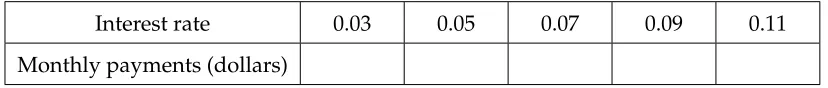
(d) Now consider only loans where the duration is 3 years. Calculate the monthly payments as indicated in Table9.2. Round payments to the nearest penny.

Interest rate 0.03 0.05 0.07 0.09 0.11

Monthly payments (dollars)

Table 9.2: Monthly payments over three years.

(e) Describe as best you can the combinations of interest rates and durations of loans that result in a monthly payment of $200.

(14)

9.1. FUNCTIONS OF SEVERAL VARIABLES AND THREE DIMENSIONAL SPACE 3

Functions of Several Variables

Suppose we launch a projectile, using a golf club, a cannon, or some other device, from ground level. Under ideal conditions (ignoring wind resistance, spin, or any other forces except the force of gravity) the horizontal distance the object will travel depends on the initial velocityxthe object is given, and the angleyat which it is launched. If we letf represent the horizontal distance the object travels (its range), thenf is a function of the two variablesxandy, and we representf in functional notation by

f(x, y) = x

2_sin(2_y₎

g ,

wheregis the acceleration due to gravity.1

Definition 9.1. Afunctionf of two independent variables is a rule that assigns to each or-dered pair(x, y)in some setDexactly one real numberf(x, y).

There is, of course, no reason to restrict ourselves to functions of only two variables—we can use any number of variables we like. For example,

f(x, y, z) =x2−2xz+ cos(y)

definesf as a function of the three variablesx,y, andz. In general, a function ofnindependent variables is a rule that assigns to an orderedn-tuple(x1, x2, . . . , xn)in some setDexactly one real

number.

As with functions of a single variable, it is important to understand the set of inputs for which the function is defined.

Definition 9.2. The domain of a function f is the set of all inputs at which the function is defined.

Activity 9.1.

Identify the domain of each of the following functions. Draw a picture of each domain in the x-yplane.

(a) f(x, y) =x2₊_y2

(b) f(x, y) =px2₊_y2

(c) Q(x, y) = _xx2+₋y_y2

(d) s(x, y) = _√ 1

1−xy2

C

(15)

Representing Functions of Two Variables

One of the techniques we use to study functions of one variable is to create a table of values. We can do the same for functions of two variables, except that our tables will have to allow us to keep track of both input variables. We can do this with a 2-dimensional table, where we list the x-values down the first column and they-values across the first row. Letfbe the function defined

byf(x, y) = x2sin(2_g y) that gives the range of a projectile as a function of the initial velocityxand

launch angleyof the projectile. The valuef(x, y)is then displayed in the location where thexrow intersects theycolumn, as shown in Table9.3(where we measurexin feet andyin radians).

x_\y 0.2 0.4 0.6 0.8 1.0 1.2 1.4

25 7.6 14.0 18.2 19.5 17.8 13.2 6.5

50 30.4 56.0 72.8 78.1 71.0 52.8 26.2

75 68.4 126.1 163.8 175.7 159.8 118.7 58.9 100 121.7 224.2 291.3 312.4 284.2 211.1 104.7 125 190.1 350.3 455.1 488.1 444.0 329.8 163.6 150 273.8 504.4 655.3 702.8 639.3 474.9 235.5 175 372.7 686.5 892.0 956.6 870.2 646.4 320.6 200 486.8 896.7 1165.0 1249.5 1136.6 844.3 418.7 225 616.2 1134.9 1474.5 1581.4 1438.5 1068.6 530.0 250

Table 9.3: Values off(x, y) = x2sin(2_g y).

Activity 9.2.

Complete the last row in Table9.3to provide the needed values of the functionf.

C Iff is a function of a single variablex, then we define the graph off to be the set of points of the form(x, f(x)), wherexis in the domain off. We then plot these points using the coordinate axes in order to visualize the graph. We can do a similar thing with functions of several variables. Table9.3identifies points of the form(x, y, f(x, y)), and we define the graph off to be the set of these points.

Definition 9.3. Thegraphof a functionf =f(x, y)is the set of points of the form(x, y, f(x, y)), where the point(x, y)is in the domain off.

(16)

9.1. FUNCTIONS OF SEVERAL VARIABLES AND THREE DIMENSIONAL SPACE 5

y-axis, and thez-axis (called thecoordinate axes). There are essentially two different ways we could set up a 3D coordinate system, as shown in Figures9.1and9.2; thus, before we can proceed, we need to establish a convention.

x

z

y

Figure 9.1: A right hand system

y

z

x

Figure 9.2: A left hand system

The distinction between these two figures is subtle, but important. In the coordinate system shown in 9.1, imagine that you are sitting on the positivez-axis next to the label “z.” Looking down at thex- andy-axes, you see that they-axis is obtained by rotating thex-axis by 90◦ in the

counterclockwisedirection. Again sitting on the positivez-axis in Figure9.2, you see that they-axis is obtained by rotating thex-axis by 90◦_{in the}_clockwise_direction.

We call the coordinate system in9.1aright-hand system; if we point the index finger of ourright

hand along the positivex-axis and our middle finger along the positivey-axis, then our thumb points in the direction of the positivez-axis. Following mathematical conventions, we choose to use a right-hand system throughout this book.

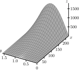
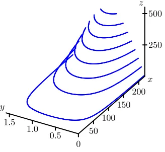
Now that we have established a convention for a right hand system, we can draw a graph of the range function defined byf(x, y) = x2sin(2_g y). Note that the functionf is continuous in both variables, so when we plot these points in the right hand coordinate system, we can connect them all to form a surface in 3-space. The graph of the range functionf is shown in Figure9.3.

There are many graphing tools available for drawing three-dimensional surfaces.2 Since we will be able to visualize graphs of functions of two variables, but not functions of more than two variables, we will primarily deal with functions of two variables in this course. It is important to note, however, that the techniques we develop apply to functions of any number of variables.

Notation:We letR2denote the set of all ordered pairs of real numbers in the plane (two copies of the real number system) and letR3 represent the set of all ordered triples of real numbers (which constitutes three-space).

2_e.g., _Wolfram _Alpha _and _{http://web.monroecc.edu/manila/webfiles/calcNSF/JavaCode/}

(17)

0 50

100 150

200

0.5 1.0 1.5

500 1000 1500

x

y

[image:17.612.226.391.109.256.2]

z

Figure 9.3: The range surface.

Some Standard Equations in Three-Space

In addition to graphing functions, we will also want to understand graphs of some simple equa-tions in three dimensions. For example, inR2, the graphs of the equationsx=aandy=b, where aandb are constants, are lines parallel to the coordinate axes. In the next activity we consider their three-dimensional analogs.

Activity 9.3.

(a) Consider the set of points(x, y, z)that satisfy the equationx = 2. Describe this set as best you can.

(b) Consider the set of points(x, y, z)that satisfy the equationy =₋1. Describe this set as best you can.

(c) Consider the set of points(x, y, z)that satisfy the equation z = 0. Describe this set as best you can.

C Activity 9.3 shows that the equations where one independent variable is constant lead to planes parallel to ones that result from a pair of the coordinate axes. When we make the con-stant 0, we get thecoordinate planes. Thexy-plane satisfiesz= 0, thexz-plane satisfiesy= 0, and theyz-plane satisfiesz= 0(see Figure9.4).

On a related note, we define a circle inR2as the set of all points equidistant from a fixed point. InR3, we call the set of all points equidistant from a fixed point asphere. To find the equation of a sphere, we need to understand how to calculate the distance between two points in three-space, and we explore this idea in the next activity.

Activity 9.4.

(18)

illus-9.1. FUNCTIONS OF SEVERAL VARIABLES AND THREE DIMENSIONAL SPACE 7

x

z

y

x

z

y

x

z

y

Figure 9.4: The coordinate planes.

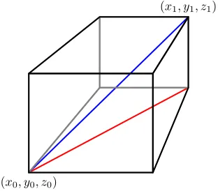
trated in Figure9.5, and the distance betweenP andQis the length of the diagonal shown in Figure9.5.

(x0, y0, z0)

(x1, y1, z1)

Figure 9.5: The distance formula inR3.

(a) Consider one of the right triangles in the base of the box whose hypotenuse is shown as the red line in Figure9.5. What are the vertices of this triangle? Since this right triangle lies in a plane, we can use the Pythagorean Theorem to find a formula for the length of the hypotenuse of this triangle. Find such a formula, which will be in terms ofx0, y0,

x1, andy1.

(b) Now notice that the triangle whose hypotenuse is the blue segment connecting the points P andQwith a leg as the hypotenuse of the triangle found in part (a) lies en-tirely in a plane, so we can again use the Pythagorean Theorem to find the length of its hypotenuse. Explain why the length of this hypotenuse, which is the distance between the pointsP andQ, is

p

(x1−x0)2+ (y1−y0)2+ (z1−z0)2.

[image:18.612.238.394.323.460.2]

(19)

The formula developed in Activity9.4is important to remember.

The distance between points P = (x0, y0, z0) andQ = (x1, y1, z1) (denoted as|P Q|) in R3 is given by the formula

|P Q_|=p(x1−x0)2+ (y1−y0)2+ (z1−z0)2. (9.2)

Equation (9.2) can be used to derive the formula for a sphere centered at a point (x0, y0, z0)

with radiusr. Since the distance from any point(x, y, z)on such a sphere to the point(x0, y0, z0)

isr, the point(x, y, z)will satisfy the equation

p

(x₋x0)2+ (y−y0)2+ (z−z0)2 =r

Squaring both sides, we come to the standard equation for a sphere.

The equation of a sphere with center(x0, y0, z0)and radiusris

(x−x0)2+ (y−y0)2+ (z−z0)2 =r2.

This makes sense if we compare this equation to its two-dimensional analogue, the equation of a circle of radiusrin the plane centered at(x0, y0):

(x−x0)2+ (y−y0)2=r2.

Traces

When we study functions of several variables we are often interested in how each individual vari-able affects the function in and of itself. In Preview Activity9.1, we saw that the monthly payment on an $18,000 loan depends on the interest rate and the duration of the loan. However, if we fix the interest rate, the monthly payment depends only on the duration of the loan, and if we set the duration the payment depends only on the interest rate. This idea of keeping one variable con-stant while we allow the other to change will be an important tool for us when studying functions of several variables.

As another example, consider again the range functionf defined by

f(x, y) = x

2_sin(2_y₎

g

wherexis the initial velocity of an object in feet per second,yis the launch angle in radians, andg is the acceleration due to gravity (32 feet per second squared). If we hold the launch angle constant aty = 0.6radians, we can considerfa function of the initial velocity alone. In this case we have

f(x) = x 2

(20)

9.1. FUNCTIONS OF SEVERAL VARIABLES AND THREE DIMENSIONAL SPACE 9

We can plot this curve on the surface by tracing out the points on the surface wheny = 0.6, as shown in Figure9.6. The graph and the formula clearly show thatfis quadratic in thex-direction. More descriptively, as we increase the launch velocity while keeping the launch angle constant, the range increases proportional to the square of the initial velocity.

Similarly, if we fix the initial velocity at 150 feet per second, we can consider the range as a function of the launch angle only. In this case we have

f(y) = 150

2_sin(2_y₎

32 .

We can again plot this curve on the surface by tracing out the points on the surface whenx= 150, as shown in Figure 9.7. The graph and the formula clearly show thatf is sinusoidal in the y-direction. More descriptively, as we increase the launch angle while keeping the initial velocity constant, the range is proportional to the sine of twice the launch angle.

0 50

100 150

200

0.5 1.0 1.5

500 1000 1500

x

y

z

Figure 9.6: The trace withy= 0.6.

0 50

100 150

200

0.5 1.0 1.5

500 1000 1500

x

y

z

Figure 9.7: The trace withx= 150.

The curves we define when we fix one of the independent variables in our two variable func-tion are calledtraces.

Definition 9.4. Atraceof a functionf of two independent variablesxandyis a curve of the formz=f(c, y)orz=f(x, c), wherecis a constant.

Understanding trends in the behavior of functions of two variables can be challenging, as can sketching their graphs; traces help us with each of these tasks.

Activity 9.5.

In the following questions, we investigate the use of traces to better understand a function through both tables and graphs.

(21)

highlighting or circling the appropriate cells in Table9.3. Write a sentence to describe the behavior of the function along this trace.

(b) Identify thex= 150trace for the range function by highlighting or circling the appro-priate cells in Table9.3. Write a sentence to describe the behavior of the function along this trace.

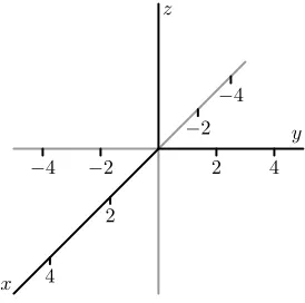
−4 −2 2 4

−4

−2

2

4

x

z

[image:21.612.242.379.197.333.2]

y

Figure 9.8: Coordinate axes to sketch traces.

(c) For the functiongdefined byg(x, y) =x2₊_y2_{+ 1}_{, explain the type of function that each}

trace in the xdirection will be (keeping yconstant). Plot they = ₋4,y = ₋2,y = 0, y= 2, andy= 4traces in 3-dimensional coordinate system provided in Figure9.8. (d) For the functiongdefined byg(x, y) =x2₊_y2_{+ 1}_{, explain the type of function that each}

trace in they direction will be (keepingx constant). Plot thex = ₋4,x = ₋2, x = 0, x= 2, andx= 4traces in 3-dimensional coordinate system in Figure9.8.

(e) Describe the surface generated by the functiong.

C

Contour Maps and Level Curves

We have all seen topographic maps such as the one of the Porcupine Mountains in the upper peninsula of Michigan shown in Figure9.9.3 The curves on these maps show the regions of con-stant altitude. The contours also depict changes in altitude: contours that are close together signify steep ascents or descents, while contours that are far apart indicate only slight changes in eleva-tion. Thus, contour maps tell us a lot about three-dimensional surfaces. Mathematically, iff(x, y)

represents the altitude at the point(x, y), then each contour is the graph of an equation of the form f(x, y) =k, for some constantk.

3_{Map source:} _{Michigan Department of Natural Resources,} _{https://www.michigan.gov/dnr/0,4570,}

(22)

Figur

e

9.9:

Contour

map

of

the

Por

cupine

[image:22.612.115.486.129.673.2]

(23)

Activity 9.6.

On the topographical map of the Porcupine Mountains in Figure9.9,

(a) identify the highest and lowest points you can find;

(b) from a point of your choice, determine a path of steepest ascent that leads to the highest point;

(c) from that same initial point, determine the least steep path that leads to the highest point.

C

Definition 9.5. Alevel curve (or contour)of a functionf of two independent variablesxand yis a curve of the formk=f(x, y), wherekis a constant.

Topographical maps can be used to create a three-dimensional surface from the two-dimensional contours or level curves. For example, level curves of the range function defined by f(x, y) =

x2_sin(2_y₎

32 plotted in thexy-plane are shown in Figure9.10. If we lift these contours and plot them

at their respective heights, then we get a picture of the surface itself, as illustrated in Figure9.11.

50 100 150 200 0.5

1.0 1.5

[image:23.612.336.500.406.557.2]

x y

Figure 9.10: Several level curves.

0 50

100 150

200

0.5 1.0 1.5

500

250

x

y

z

Figure 9.11: Level curves at the ap-propriate height.

The use of level curves and traces can help us construct the graph of a function of two variables.

Activity 9.7.

(a) Letf(x, y) = x2 ₊_y2_{. Draw the level curves} _f₍_{x, y}_{) =} _k_for_k _{= 1}_,_k _{= 2}_, _k _{= 3}_{, and}

(24)

x y

Figure 9.12: Left: Level curves forf(x, y) =x2₊_y2_{. Right: Level curves for}_g₍_{x, y}_{) =}p

x2₊_y2_.

(b) Letg(x, y) =px2₊_y2_{. Draw the level curves}_g₍_{x, y}_{) =}_k_for_k _{= 1}_,_k_{= 2}_,_k _{= 3}_{, and}

k= 4on the right set of axes given in Figure9.12. (You decide on the scale of the axes.) Explain what the surface defined byglooks like.

(c) Compare and contrast the graphs off andg. How are they alike? How are they differ-ent? Use traces for each function to help answer these questions.

C The traces and level curves of a function of two variables are curves in space. In order to understand these traces and level curves better, we will first spend some time learning about vectors and vector-valued functions in the next few sections and return to our study of functions of several variables once we have those more mathematical tools to support their study.

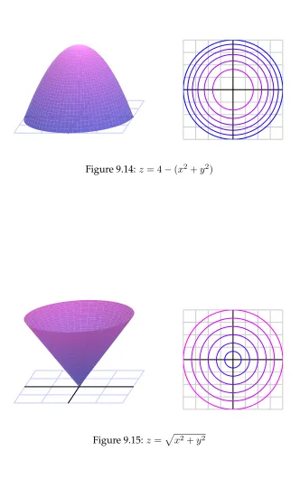
A gallery of functions

We end this section by considering a collection of functions and illustrating their graphs and some level curves.

(25)

[image:25.612.148.480.145.696.2]

Figure 9.14:z= 4₋(x2₊_y2₎

(26)

x y

z

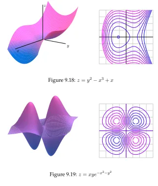
Figure 9.16:z=x2₋_y2

(27)

x

[image:27.612.148.471.111.491.2]

y z

Figure 9.18:z=y2₋_x3₊_x

Figure 9.19:z=xye−x2₋_y2

Summary

• A functionf of several variables is a rule that assigns a unique number to an ordered collection of independent inputs. The domain of a function of several variables is the set of all inputs for which the function is defined.

• In R3, the distance between pointsP = (x0, y0, z0) and Q = (x1, y1, z1) (denoted as|P Q|) is

given by the formula

|P Q|=p(x1−x0)2+ (y1−y0)2+ (z1−z0)2.

and thus the equation of a sphere with center(x0, y0, z0)and radiusris

(x−x0)2+ (y−y0)2+ (z−z0)2 =r2.

• A trace of a functionf of two independent variablesxandyis a curve of the formz=f(c, y)

(28)

9.1. FUNCTIONS OF SEVERAL VARIABLES AND THREE DIMENSIONAL SPACE 17

• A level curve of a function f of two independent variables x and y is a curve of the form k = f(x, y), where k is a constant. A level curve describes the set of inputs that lead to a specific output of the function.

Exercises

1. Find the equation of each of the following geometric objects.

(a) The plane parallel to thex-yplane that passes through the point(₋4,5,₋12).

(b) The plane parallel to they-zplane that passes through the point(7,₋2,₋3).

(c) The sphere centered at the point(2,1,3)and has the point(−1,0,−1)on its surface.

(d) The sphere whose diameter has endpoints(₋3,1,₋5)and(7,9,₋1).

2. The Ideal Gas Law,P V =RT, relates the pressure (P, in pascals), temperature (T, in Kelvin), and volume (V, in cubic meters) of 1 mole of a gas (R = 8.314 _{mol K}J is the universal gas con-stant), and describes the behavior of gases that do not liquefy easily, such as oxygen and hy-drogen. We can solve the ideal gas law for the volume and hence treat the volume as a function of the pressure and temperature:

V(P, T) = 8.314T

P .

(a) Explain in detail what the trace ofV withP = 1000tells us about a key relationship between two quantities.

(b) Explain in detail what the trace ofV withT = 5tells us.

(c) Explain in detail what the level curveV = 0.5tells us.

(d) Use 2 or three additional traces in each direction to make a rough sketch of the surface over the domain ofV wherePandT are each nonnegative. Write at least one sentence that describes the way the surface looks.

(e) Based on all your work above, write a couple of sentences that describe the effects that temperature and pressure have on volume.

3. Consider the functionhdefined byh(x, y) = 8−p

4−x2₋_y2_.

(a) What is the domain ofh? (Hint: describe a set of ordered pairs in the plane by explain-ing their relationship relative to a key circle.)

(b) Therangeof a function is the set of all outputs the function generates. Given that the range of the square root functiong(t) = √tis the set of all nonnegative real numbers, what do you think is the range ofh? Why?

(29)

(d) Choose 5 different values of x (including at least one negative value and zero), and sketch the corresponding traces of the functionh.

(e) Choose 5 different values of y (including at least one negative value and zero), and sketch the corresponding traces of the functionh.

(30)

9.2. VECTORS 19

9.2

Vectors

Motivating Questions

• What is a vector?

• What does it mean for two vectors to be equal?

• How do we add two vectors together and multiply a vector by a scalar?

• How do we determine the magnitude of a vector? What is a unit vector, and how do we find a unit vector in the direction of a given vector?

Introduction

If we are at a pointxin the domain of a function of one variable, there are only two directions in which we can move: in the positive or negativex-direction. If, however, we are at a point(x, y)in the domain of a function of two variables, there are many directions in which we can move. Thus, it is important for us to have a means to indicate direction, and we will do so using vectors.

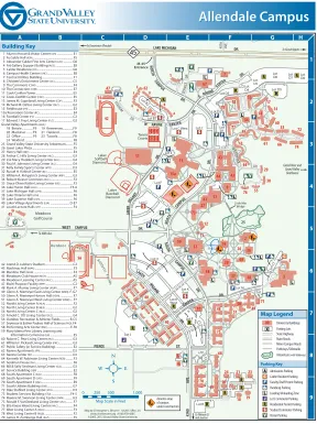
Preview Activity 9.2. After working out, Sarah and John leave the Recreation Center on the Grand Valley State University Allendale campus (a map of which is given in Figure9.20) to go to their next classes.4 Suppose we record Sarah’s movement on the map in a pairhx, y_i(we will call this pair a vector), where x is the horizontal distance (in feet) she moves (with east as the positive direction) andyas the vertical distance (in feet) she moves (with north as the positive direction). We do the same for John. Throughout, use the legend to estimate your responses as best you can.

(a) What is the vectorv1 = hx, yithat describes Sarah’s movement if she walks directly in a

straight line path from the Recreation Center to the entrance at the northwest end of Mack-inac Hall? (Assume a straight line path, even if there are buildings in the way.) Explain how you found this vector. What is the total distance in feet between the Recreation Center and the entrance to Mackinac Hall? Measure the number of feet directly and then explain how to calculate this distance in terms ofxandy.

(b) What is the vectorv2 =hx, yithat describes John’s change in position if he walks directly

from the Recreation Center to Au Sable Hall? How many feet are there between Recreation Center to Au Sable Hall in terms ofxandy?

(c) What is the vectorv3 = hx, yithat describes the change in position if John walks directly

from Au Sable Hall to the northwest entrance of Mackinac Hall to meet up with Sarah after

4_{GVSU campus map from}_{http://www.gvsu.edu/homepage/files/pdf/maps/allendale.pdf}_{, used with}

(31)

class? What relationship do you see among the vectorsv1, v2, andv3? Explain why this

relationship should hold.

./ Lot J Lot R Lot K East Lot K West Lot H Lot M Lot O Lot L Lot G Lot E Lot C West Lot B1 Lot C Lot A Lot B2 Lot D1 Lot D6 Lot D5 Lot D4 Lot D7 LotD8 Lot D9 52 78 34 77 13 35 53 17 14 54 61 33 ₇₂ 66 ₇₄ 28 29 30 55 76 43 43 44 9 27 73 12 32 59 58 79 2 39 37 65 36 38 5 3 71 48 75 20 24 21 22 18 19 23 40 40 8 15 11

WEST CAMPUS DR.

LA KE R VILL AGE DR. LAKER V ILLAG E D R. ST AD IUM D R.

W. RAVINE CENTER DR. NO RTH C AM PU S DR. N ORTH CAM PUS D R. SO UT H C AM PU S DR .

42ND AVE.

PIERCE ST. SE RV ICE D R.

LAKE MICHIGAN DR.

63 A B C D E F G H 47 16 1 67 7

1 Alumni House & Visitor Center (AH)...E1 2 Au Sable Hall (ASH)... F5 3 Alexander Calder Fine Arts Center (CAC)... G6 4 Art Gallery Support Building (AGS)...E8 5 Calder Residence (CR)... G6 6 Campus Health Center (UHC)...E8 7 Central Utilities Building... F1 8 Children’s Enrichment Center (CC)...C5 9 The Commons (COM)... F4 10 The Connection (CON)...E7 11 Cook Carillon Tower...E5 12 Cook–DeWitt Center (CDC)...E5 13 James M. Copeland Living Center (COP)... F3 14 Richard M. DeVos Living Center (DLC)... G2 15 Fieldhouse (FH)...E3 15a Recreation Center (RC)...E4 16 Football Center (FC)...C2 17 Edward J. Frey Living Center (FLC)... G2 Grand Valley Apartments (GVA): 18 Benzie...F9 19 Keweenaw...F9 20 Mackinac ...F9 21 Oakland...F8 22 Office ...F9 23 Tuscola ...F8 24 Wexford ... F8 25 Grand Valley State University Arboretum... F5 26 Great Lakes Plaza... F5 27 Henry Hall (HRY)...E4 28 Arthur C. Hills Living Center (HLC)... G3 29 Icie Macy Hoobler Living Center (HLL)... G4 30 Paul A. Johnson Living Center (JLC)... G4 31 Kelly Family Sports Center (KTB)... D3 32 Russel H. Kirkhof Center (KC)...E5 33 William A. Kirkpatrick Living Center (KRP)... G3 34 Robert Kleiner Commons (KLC)... F2 35 Grace Olsen Kistler Living Center (KIS)... F3 36 Lake Huron Hall (LHH)... F5-6 37 Lake Michigan Hall (LHM)... F6 38 Lake Ontario Hall (LOH)... F6 39 Lake Superior Hall (LSH)... F6 40 Laker Village Apartments (LVA)... D-E7 41 Loutit Lecture Halls (LTT)... F4

42 Arend D. Lubbers Stadium...C2 43 Mackinac Hall (MAK)... F3 44 Manitou Hall (MAN)... F4 45 Meadows Club House (MCH)... A5 46 Meadows Learning Center (MLC)... A5 47 Multi-Purpose Facility (MPF)...C2 48 Mark A. Murray Living Center (MUR)... F7 49 Glenn A. Niemeyer East Living Center (NMR). F-G7 50 Glenn A. Niemeyer Honors Hall (HON)... F7 51 Glenn A. Niemeyer West Living Center (NMR).... F7 52 North Living Center A (NLA)... F2 53 North Living Center B (NLB)... G2 54 North Living Center C (NLC)... G2 55 Arnold C. Ott Living Center (OLC)... G4 56 Outdoor Recreation & Athletic Fields... B-C5 57 Seymour & Esther Padnos Hall of Science (PAD). F4 58 Performing Arts Center (PAC)... E-F6 59 Mary Idema Pew Library Learning and

Information Commons (LIB)...E5 60 Robert C. Pew Living Center (PLC)... G3 61 William F. Pickard Living Center (PKC)... G3 67 Public Safety (in Service Building)...E2 62 Ravine Apartments (RA)... D2 63 Ravine Center (RC)... D2 64 Kenneth W. Robinson Living Center (ROB)... F3 65 Seidman House (SH)... F6 66 Bill & Sally Seidman Living Center (SLC)... G3 67 Service Building (SER)...E2 68 South Apartment C (SAC)... F8 69 South Apartment D (SAD)... F9 70 South Apartment E (SAE)...E9 71 South Utilities Building (SUB)... G7 72 Dale Stafford Living Center (STA)... H3 73 Student Services Building (STU)... F4-5 74 Maxine M. Swanson Living Center (SWN)... H3 75 Ronald F. VanSteeland Living Center (VLC)... F7 76 Ella Koeze Weed Living Center (WLC)... F4 77 West Living Center A (WLA)... F3 78 West Living Center B (WLB)... F2 79 James H. Zumberge Hall (JHZ)... F5

45 46 Building Key 62 60 64 42 41 25

Grand River and Grand Valley Boathouse Little Mac Bridge Map Legend University Buildings Parking Lots State Highway Main Roads Minor Campus Roads Pathways/Sidewalks Arboretum (with Walkway)

Tennis Courts Laker Softball Diamond Laker Baseball Diamond WT 6 15a 57 Meadows Golf Course

0 250 500 1,000 Map Scale in Feet

Lot P 26 50 51 49 Lot N RE

SIDEN CE

DR.

31

E

. RAVIN E CE

NTER DR . 00 40TH AVE. M-45 Entrance

To Grand Rapids To Downtown Allendale

To Fillmore St and Jenison Lot D2 Lot D3 10 68 70 69 56

To 48th Ave.

4

Zumberge Pond

Outdoor Recreatio_{n a}

nd A th_le tic F ie_ld s Lot F J C Parking Key Admissions Parking Calder Resident Parking Faculty/Staff Permit Parking Handicap Parking Loading/Unloading Zone Lot J Commuter Parking Residential Permit Parking Student Commuter Parking Visitor Parking C

J

CALD

ER DR.

denotes areas of campus under construction

Allendale Campus

C B

A D E F G H

[image:31.612.170.458.237.622.2]

Allendale Campus

1 2 3 4 5 6 7 8 9

(32)

9.2. VECTORS 21

Representations of Vectors

Preview Activity9.2 shows how we can record the magnitude and direction of a change in po-sition using an ordered pair of numbers hx, yi. There are many other quantities, such as force and velocity, that possess the attributes of magnitude and direction, and we will call each such quantity avector.

Definition 9.6. Avectoris any quantity that possesses the attributes of magnitude and direc-tion.

We can represent a vector geometrically as a directed line segment, with the magnitude as the length of the segment and an arrowhead indicating direction, as shown in Figure9.21.

Figure 9.21: A vector. Figure 9.22: Representations of the same vector.

According to the definition, a vector possesses the attributes of length (magnitude) and direc-tion; the vector’s position, however, is not mentioned. Consequently, we regard as equal any two vectors having the same magnitude and direction, as shown in Figure9.22.

Two vectors are equal provided they have the same magnitude and direction.

This means that the same vector may be drawn in the plane in many different ways. For instance, suppose that we would like to draw the vector h3,4i, which represents a horizontal change of three units and a vertical change of four units. We may place thetailof the vector (the point from which the vector originates) at the origin and thetip(the terminal point of the vector) at(3,4), as illustrated in Figure9.23. A vector with its tail at the origin is said to be instandard position.

(33)

3 4

x y

Figure 9.23: A vector in standard position

1 4

1 5

x y

Q(1,1)

R(4,5)

Figure 9.24: A vector between two points

In this example, the vector led to the directed line segment fromQtoR, which we denote as

−−→

QR. We may also turn the situation around: given the two pointsQandR, we obtain the vector

h3,4_ibecause we move horizontally three units and vertically four units to get from Qto R. In other words,−−→QR =_h3,4_i. In general, the vector−−→QRfrom the pointQ= (q1, q2)toR = (r1, r2)is

found by taking the difference of coordinates, so that

−−→

QR=_hr1−q1, r2−q2i.

We will use boldface letters to represent vectors, such asv =_h3,4_i, to distinguish them from scalars. The entries of a vector are called itscomponents; in the vectorh3,4i, thexcomponent is 3 and theycomponent is 4. We use pointed bracketsh,_iand the termcomponentsto distinguish a vector from a point(,)and itscoordinates. There is, however, a close connection between vectors and points. Given a pointP, we will frequently consider the vector−−→OP from the originO toP. For instance, ifP = (3,4), then−−→OP =_h3,4_ias in Figure9.25. In this way, we think of a pointP as defining a vector−−→OP whose components agree with the coordinates ofP.

x y

P(3,4)

−−→

OP =h3,4i

Figure 9.25: A point defines a vector

(34)

n-9.2. VECTORS 23

dimensional space,Rn, hasncomponents and may be represented as

v=_hv1, v2, v3, . . . , vni.

The next activity will help us to become accustomed to vectors and operations on vectors in three dimensions.

Activity 9.8.

As a class, determine a coordinatization of your classroom, agreeing on some convenient set of axes (e.g., an intersection of walls and floor) and some units in thex,y, andzdirections (e.g., using lengths of sides of floor, ceiling, or wall tiles). Let O be the origin of your coordinate system. Then, choose three points,A,B, andCin the room, and complete the following.

(a) Determine the coordinates of the pointsA,B, andC.

(b) Determine the components of the indicated vectors.

(i)−→OA (ii)−−→OB (iii)−−→OC (iv)−−→AB (v)−→AC (vi)−−→BC

C

Equality of Vectors

Because location is not mentioned in the definition of a vector, any two vectors that have the same magnitude and direction are equal. It is helpful to have an algebraic way to determine when this occurs. That is, if we know the components of two vectorsu andv, we will want to be able to determine algebraically whenuandvare equal. There is an obvious set of conditions that we use.

Two vectors u = hu1, u2i andv = hv1, v2iin R2 are equal if and only if their corresponding components are equal: u1 =v1 andu2 =v2. More generally, two vectorsu =hu1, u2, . . . , uni

andv=_hv1, v2, . . . , vniinRnare equal if and only ifui =vifor each possible value ofi.

Operations on Vectors

Vectors are not numbers, but we can now represent them with components that are real numbers. As such, we naturally wonder if it is possible to add two vectors together, multiply two vectors, or combine vectors in any other ways. In this section, we will study two operations on vectors: vector addition and scalar multiplication. To begin, we investigate a natural way to add two vectors together, as well as to multiply a vector by a scalar.

Activity 9.9.

Letu=_h2,3_i,v=_h−1,4_i.

(a) Using the two specific vectors above, what is the natural way to define the vector sum

(35)

(b) In general, how do you think the vector suma+bof vectorsa=_ha1, a2iandb=hb1, b2i

in R2 should be defined? Write a formal definition of a vector sum based on your intuition.

(c) In general, how do you think the vector sum a+b of vectors a = _ha1, a2, a3i and

b = hb1, b2, b3i in R3 should be defined? Write a formal definition of a vector sum based on your intuition.

(d) Returning to the specific vector v = h−1,4i given above, what is the natural way to define the scalar multiple 1₂v?

(e) In general, how do you think a scalar multiple of a vectora=_ha1, a2iinR2by a scalar cshould be defined? how about for a scalar multiple of a vectora =ha1, a2, a3iinR3 by a scalarc? Write a formal definition of a scalar multiple of a vector based on your intuition.

C We can now add vectors and multiply vectors by scalars, and thus we can add together scalar multiples of vectors. This allows us to definevector subtraction,v−u, as the sum ofvand−1times

u, so that

v−u=v+ (−1)u.

Using vector addition and scalar multiplication, we will often represent vectors in terms of the special vectorsi=_h1,0_iandj=_h0,1_i. For instance, we can write the vectorha, b_iinR2as

ha, b_i=a_h1,0_i+b_h0,1_i=ai+bj,

which means that

h2,₋3_i= 2i₋3j.

In the context ofR3, we leti=h1,0,0i,j=h0,1,0i, andk=h0,0,1i, and we can write the vector

ha, b, c_iinR3as

ha, b, c_i=a_h1,0,0_i+b_h0,1,0_i+c_h0,0,1_i=ai+bj+ck.

The vectorsi, j, andkare called thestandard unit vectors5_{, and are important in the physical}

sci-ences.

Properties of Vector Operations

We know that the scalar sum1 + 2is equal to the scalar sum2 + 1. This is called thecommutative

property of scalar addition. Any time we define operations on objects (like addition of vectors) we usually want to know what kinds of properties the operations have. For example, is addition of vectors a commutative operation? To answer this question we take twoarbitraryvectorsvandu

(36)

9.2. VECTORS 25

and add them together and see what happens. Letv=_hv1, v2iandu =hu1, u2i. Now we use the

fact thatv1,v2,u1, andu2are scalars, and that the addition of scalars is commutative to see that

v+u=_hv1, v2i+hu1, u2i=hv1+u1, v2+u2i=hu1+v1, u2+v2i=hu1, u2i+hv1, v2i=u+v.

So the vector sum is a commutative operation. Similar arguments can be used to show the follow-ing properties of vector addition and scalar multiplication.

Letv,u, andwbe vectors inRnand letaandbbe scalars. Then

1. v+u=u+v

2. (v+u) +w=v+ (u+w)

3. The vector0 = _h0,0, . . . ,0_ihas the property thatv+0 = v. The vector0is called the

zero vector.

4. (₋1)v+v=0. The vector(₋1)v=₋vis called theadditive inverseof the vectorv.

5. (a+b)v=av+bv

6. a(v+u) =av+au

7. (ab)v=a(bv)

8. 1v=v.

We verified the first property for vectors inR2; it is straightforward to verify that the rest of the eight properties just noted hold for all vectors inRn.

Geometric Interpretation of Vector Operations

Next, we explore a geometric interpretation of vector addition and scalar multiplication that al-lows us to visualize these operations. Letu=_h4,6_iandv=_h3,₋2_i. Thenw=u+v=_h7,4_i, as shown on the left in Figure9.26.

If we think of these vectors as displacements in the plane, we find a geometric way to envision vector addition. For instance, the vectoru+vwill represent the displacement obtained by follow-ing the displacementuwith the displacementv. We may picture this by placing the tail ofvat the tip ofu, as seen in the center of Figure9.26.

Of course, vector addition is commutative so we obtain the same sum if we place the tail ofu

at the tip ofv. We therefore see thatu+vappears as the diagonal of the parallelogram determined byuandv, as shown on the right of Figure9.26.

(37)

v u

u+v

v

u

u+v

v u

u+v

Figure 9.26: A vector sum (left), summing displacements (center), the parallelogram law (right)

v

u

w=u+v

Figure 9.27: Vector addition

w−u

u

w

Figure 9.28: Vector subtraction

(38)

9.2. VECTORS 27

v 2v

[image:38.612.84.517.74.562.2]

−2v

Figure 9.29: Scalar multiplication

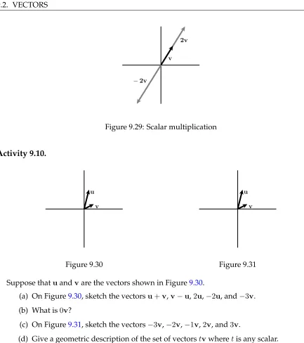
Activity 9.10.

v u

Figure 9.30

v u

Figure 9.31

Suppose thatuandvare the vectors shown in Figure9.30.

(a) On Figure9.30, sketch the vectorsu+v,v−u,2u,−2u, and−3v. (b) What is0v?

(c) On Figure9.31, sketch the vectors−3v,−2v,−1v,2v, and3v.

(d) Give a geometric description of the set of vectorstvwheretis any scalar.

(e) On Figure9.31, sketch the vectorsu₋3v,u₋2v,u₋v,u+v, andu+ 2v. (f) Give a geometric description of the set of vectorsu+tvwheretis any scalar.

C

The Magnitude of a Vector

(39)

we can use the distance formula to calculate the length of the segment. This length is themagnitude

of the vectorvand is denoted|v_|.

Activity 9.11.

2 4

3 7

A B

x y

Figure 9.32: The vector defined byAandB.

v

v1

v2

(v1, v2)

x y

Figure 9.33: An arbitrary vector,v.

(a) LetA= (2,3)andB= (4,7), as shown in Figure9.32. Compute|−−→AB|.

(b) Letv=_hv1, v2ibe the vector inR2with componentsv1 andv2 as shown in Figure9.33.

Use the distance formula to find a general formula for|v|.

(c) Letv=_hv1, v2, v3ibe a vector inR3. Use the distance formula to find a general formula for|v|.

(d) Suppose that u = _h2,3_i and v = _h−1,2_i. Find |u_|, |v_|, and |u+v_|. Is it true that

|u+v|=|u|+|v|?

(e) Under what conditions will|u+v_|=_|u_|+_|v_|? (Hint: Think about howu,v, andu+v

form the sides of a triangle.)

(f) With the vectoru = _h2,3_i, find the lengths of 2u, 3u, and −2u, respectively, and use proper notation to label your results.

(g) Iftis any scalar, how is_|tu_|related to_|u_|?

(h) Aunit vectoris a vector whose magnitude is 1. Of the vectorsi,j, andi+j, which are unit vectors?

(i) Find a unit vectorvwhose direction is the same asu=_h2,3_i. (Hint: Consider the result of part (g).)

C

Summary

(40)

9.2. VECTORS 29

• Two vectors are equal if they have the same direction and magnitude. Notice that position is not considered, so a vector is independent of its location.

• Ifu = hu1, u2, . . . , uniandv = hv1, v2, . . . , vni are two vectors inRn, then their vector sum is the vector

u+v=_hu1+v1, u2+v2, . . . , un+vni.

Ifu=_hu1, u2, . . . , uniis a vector inRnandcis a scalar, then the scalar multiplecuis the vector

cu=_hcu1, cu2, . . . , cuni.

• The magnitude of the vectorv=_hv1, v2, . . . , vniinRnis the scalar

|v_|=

q

v2

1+v22+· · ·+vn2.

A vectoruis a unit vector provided that|u_|= 1. Ifvis a nonzero vector, then the vector _|v_v_| is a unit vector with the same direction asv.

Exercises

1. Letv=_h1,₋2_i,u=_h0,4_i, andw=_h−5,7_i.

(a) Determine the components of the vectoru₋v.

(b) Determine the components of the vector2v−3u.

(c) Determine the components of the vectorv+ 2u−7w.

(d) Determine scalarsaandbsuch thatav+bu=w.

2. Letu=h2,1iandv=h1,2i.

(a) Determine the components and draw geometric representations of the vectors2u, 1₂u,

(₋1)u, and(₋3)uon the same set of axes.

(b) Determine the components and draw geometric representations of the vectorsu+v,

u+ 2v, andu+ 3v.

(c) Determine the components and draw geometric representations of the vectorsu−v,

u₋2v, andu₋3v.

(d) Recall thatu₋v = u+ (₋1)v. Use the “tip to tail” perspective for vector addition to explain why the differenceu−vcan be viewed as a vector that points from the tip ofv

to the tip ofu.

(41)

(a) Letv=_h3,4_iinR2. Compute|v|, and determine the components of the vectoru= |v1|v.

What is the magnitude of the vectoru? How does its direction compare tov?

(b) Letw= 3i₋3jinR2. Determine a unit vectoruin the same direction asw.

(c) Letv = _h2,3,5_iinR3. Compute|v|, and determine the components of the vectoru =

1

|v|v. What is the magnitude of the vectoru? How does its direction compare tov?

(42)

9.3. THE DOT PRODUCT 31

9.3

The Dot Product

Motivating Questions

• How is the dot product of two vectors defined and what geometric information does it tell us?

• How can we tell if two vectors inRnare perpendicular?

• How do we find the projection of one vector onto another?

Introduction

In the last section, we considered vector addition and scalar multiplication and found that each operation had a natural geometric interpretation. In this section, we will introduce a means of multiplying vectors.

Preview Activity 9.3. For two-dimensional vectorsu =_hu1, u2iandv=hv1, v2i, the dot product

is simply the scalar obtained by

u·v=u1v1+u2v2.

(a) Ifu=h3,4iandv=h−2,1i, find the dot productu·v.

(b) Findi·iandi·j.

(c) Ifu=_h3,4_i, findu_·u. How is this related to|u_|?

(d) On the axes in Figure9.34, plot the vectorsu = _h1,3_iandv = _h−3,1_i. Then, find u_·v. What is the angle between these vectors?

-4 -2 2 4

[image:42.612.254.370.535.656.2]

x y

(43)

-4 -2 2 4

[image:43.612.254.371.106.227.2]

x y

Figure 9.35: For part (e)

(e) On the axes in Figure9.35, plot the vectoru=h1,3i.

For each of the following vectorsv, plot the vector on Figure 9.35and then compute the dot productu·v.

• v=_h3,2_i.

• v=_h3,0_i.

• v=_h3,₋1_i.

• v=h3,−2i.

• v=h3,−4i.

(f) Based upon the previous part of this activity, what do you think is the sign of the dot product in the following three cases shown in Figure9.36?

v

u

v

u

v

u

Figure 9.36: For part (f)

(44)

9.3. THE DOT PRODUCT 33

The Dot Product

If we have twon-dimensional vectorsu=_hu1, u2, . . . , uniandv=hv1, v2, . . . , vni, we define their

dot product6_as

u_·v=u1v1+u2v2+. . .+unvn.

For instance, we find that

h3,0,1_{i · h−}2,1,4_i= 3_·(₋2) + 0_·1 + 1_·4 =₋6 + 0 + 4 =₋2.

Notice that the resulting quantity is a scalar. Our work in Preview Activity 9.3 examined dot products of two-dimensional vectors.

Activity 9.12.

Determine each of the following.

(a) h1,2,₋3_{i · h}4,₋2,0_i.

(b) h0,3,₋2,1_{i · h}5,₋6,0,4_i

C The dot product is a natural way to define a product of two vectors. In addition, it behaves in ways that are similar to the product of, say, real numbers.

Letu,v, andwbe vectors inRn. Then

(a) u_·v=v_·u(the dot product iscommutative), and

(b) ifcis a scalar, then(cu+v)_·w=c(u_·w) +v_·w(the dot product isbilinear),

Moreover, the dot product gives us valuable geometric information about the vectors and their relative orientation. For instance, let’s consider what happens when we dot a vector with itself:

u_·u=_hu1, u2, . . . , uni · hu1, u2, . . . , uni=u21+u22+. . .+u2n=|u|2.

In other words, the dot product of a vector with itself gives the square of the length of the vector:

u·u=|u|2_.

The angle between vectors

The dot product can help us understand the angle between two vectors. For instance, if we are given two vectorsu andv, there are two angles that these vectors create, as depicted in Figure

9.37. We will call θ, the smaller of these angles, theangle between these vectors. Notice thatθ lies between 0 andπ.

6_{As we will see shortly, the dot product arises in physics to calculate the work done by a vector force in a given}

(45)

u v

θ

2π−θ

Figure 9.37: The angle between vectorsu

andv.

v u

θ

u−v

Figure 9.38: The triangle formed byu,v, and

u₋v.

To determine this angle, we may apply the Law of Cosines to the triangle shown in Figure9.38. Using the fact that the dot product of a vector with itself gives us the square of its length, together with the bilinearity of the dot product, we find:

|u−v|2 ₌ _|_u_|2₊_|_v_|2₋₂_|_u_||_v_|_cos(_θ₎

(u−v)·(u−v) = u·u+v·v−2|u||v|cos(θ)

u_·(u₋v)₋v_·(u₋v) = u_·u+v_·v₋2_|u_||v_|cos(θ)

u_·u₋2u_·v+v_·v = u_·u+v_·v₋2_|u_||v_|cos(θ)

−2u_·v = ₋2_|u_||v_|cos(θ)

u·v = |u||v|cos(θ).

To summarize, we have the important relationship

u·v=u1v1+u2v2+. . .+unvn=|u||v|cos(θ). (9.3)

It is sometimes useful to think of Equation (9.3) as giving us an expression for the angle be-tween two vectors:

θ= cos−1

u_·v |u||v|

.

The real beauty of this expression is this: the dot product is a very simple algebraic operation to perform yet it provides us with important geometric information – namely the angle between the vectors – that would be difficult to determine otherwise.

Activity 9.13.

Determine each of the following.

(a) The length of the vectoru=_h1,2,₋3_iusing the dot product.

(46)

9.3. THE DOT PRODUCT 35

(c) The angle between the vectorsy=_h1,2,₋3_iandz=_h−2,1,1_ito the nearest tenth of a degree.

(d) If the angle between the vectors u and v is a right angle, what does the expression

u·v=|u||v|cosθsay about their dot product?

(e) If the angle between the vectorsuandvis acute—that is, less thanπ/2—what does the expressionu·v=|u||v|cosθsay about their dot product?

(f) If the angle between the vectorsuandvis obtuse—that is, greater thanπ/2—what does the expressionu·v=|u||v|cosθsay about their dot product?

C

The Dot Product and Orthogonality

When the angle between two vectors is a right angle, it is frequently the case that something important is happening. In this case, we say the vectors areorthogonal. For instance, orthogonality often plays a role in optimization problems; to determine the shortest path from a point inR3to a given plane, we move along a line orthogonal to the plane.

As Activity9.13indicates, the dot product provides a simple means to determine whether two vectors are orthogonal to one another. In this case, u_·v = _|u_||v_|cos(π/2) = 0, so we make the following important observation.

Two vectorsuandvinRnare orthogonal to each other ifu·v= 0.

More generally, the sign of the dot product gives us useful information about the relative ori-entation of the vectors. If we remember that

cos(θ)>0 ifθis an acute angle,

cos(θ) = 0 ifθis a right angle,

andcos(θ)<0 ifθis an obtuse angle,

we see that

u·v>0 ifθis an acute angle,

u_·v= 0 ifθis a right angle, andu·v<0 ifθis an obtuse angle.

(47)

v

u

u·v>0

v

u

u·v= 0

v

u

u·v<0

Figure 9.39: The orientation of vectors

Work, Force, and Displacement

In physics, work is a measure of the energy required to apply a force to an object through a dis-placement. For instance, Figure9.40shows a forceFdisplacing an object from pointAto pointB. The displacement is then represented by the vector−−→AB.

|F|cosθ

A θ B

F

Figure 9.40: A forceFdisplacing an object.

It turns out that the work required to displace the object is

W =F_·−−→AB=_|F_||−−→AB_|cos(θ).

This means that the work is determined only by the magnitude of the force applied parallel to the displacement. Consequently, if we are given two vectorsu andv, we would like to writeu as a sum of two vectors, one of which is parallel tovand one of which is orthogonal tov. We take up this task after the next activity.

Activity 9.14.

Determine the work done by a 25 pound force acting at a 30◦ angle to the direction of the object’s motion, if the object is pulled 10 feet. In addition, is more work or less work done if the angle to the direction of the object’s motion is60◦_?

(48)

9.3. THE DOT PRODUCT 37

Projections

v u

θ

projvu

proj_⊥vu

Figure 9.41: The projection ofuontov.

v u

θ

projvu

proj_⊥vu

Figure 9.42: proj_vuwhenθ > π₂.

Suppose we are given two vectorsuandvas shown in Figure9.41. Motivated by our discus-sion of work, we would like to writeuas a sum of two vectors, one of which is parallel tovand one of which is orthogonal. That is, we would like to write

u=proj_vu+proj_⊥_vu, (9.4)

where proj_vuis parallel tovand proj_⊥_vuis orthogonal tov. We call the vector proj_vutheprojection

ofuontov.

To find the vector proj_vu, we will dot both sides of Equation (9.4) with the vectorv, to find that

u_·v = (proj_vu+proj_⊥_vu)_·v

= (proj_vu)_·v+ (proj_⊥_vu)_·v

= (proj_vu)·v.

Notice that (proj_⊥_vu) _·v = 0 since proj_⊥_vu is orthogonal to v. Also, proj_vu must be a scalar multiple ofvsince it is parallel tov, so we will write proj_vu=sv. It follows that

u_·v= (proj_vu)_·v=sv_·v,

which means that

s= u·v

v·v

and hence

proj_vu= u·v

v_·vv= u·v

|v_|2 v

It is sometimes useful to write proj_vuas a scalar times a unit vector in the direction ofv. We call this scalar thecomponent ofualongvand denote it as comp_vu. We therefore have

proj_vu= u·v

|v_|2 v=

u_·v |v_|

v

|v_| =compvu

(49)

so that

comp_vu= u·v

|v| .

Letuandvbe vectors inRn. The component ofuin the direction ofvis the scalar

comp_vu= u·v

|v| ,

and the projection ofuontovis the vector

pro

Active Calculus Multivariable

MULTIVARIABLE

Contents

Preface v

Preface

Active Calculus - Multivariable: our goals

Features of the Text

How to Use this Text

Electronically

Community of Users

Acknowledgments

Chapter 9

Motivating Questions

Introduction

9.1. FUNCTIONS OF SEVERAL VARIABLES AND THREE DIMENSIONAL SPACE 3

Activity 9.1.

Activity 9.2.

Some Standard Equations in Three-Space

Activity 9.4.

Traces

9.1. FUNCTIONS OF SEVERAL VARIABLES AND THREE DIMENSIONAL SPACE 9

Activity 9.5.

Contour Maps and Level Curves

Activity 9.6.

Activity 9.7.

A gallery of functions

9.1. FUNCTIONS OF SEVERAL VARIABLES AND THREE DIMENSIONAL SPACE 17

9.2. VECTORS 19

Vectors

Motivating Questions

Introduction

WEST CAMPUS DR.

LA KE R VILL AGE DR. LAKER V ILLAG E D R. ST AD IUM D R.

W. RAVINE CENTER DR. NO RTH C AM PU S DR. N ORTH CAM PUS D R. SO UT H C AM PU S DR .

PIERCE ST. SE RV ICE D R.

LAKE MICHIGAN DR.

45 46 Building Key 62 60 64 42 41 25

SIDEN CE

. RAVIN E CE

Allendale Campus

9.2. VECTORS 21

Activity 9.8.

Equality of Vectors

Activity 9.9.

Properties of Vector Operations

Geometric Interpretation of Vector Operations

9.2. VECTORS 27

The Magnitude of a Vector

Summary

Exercises

9.3. THE DOT PRODUCT 31

The Dot Product

Motivating Questions

Introduction

9.3. THE DOT PRODUCT 33

Activity 9.12.

The angle between vectors

Activity 9.13.

The Dot Product and Orthogonality

Work, Force, and Displacement

Activity 9.14.