Phylogenetic Comparative Methods
Luke J. Harmon
Copyright
This is book version 1.4, released 15 March 2019.
This book is released under a CC-BY-4.0 license. Anyone is free to share and adapt this work with attribution.
Acknowledgements
Thanks to my lab for inspiring me, my family for being my people, and to the students for always keeping us on our toes.
Helpful comments on this book came from many sources, including Arne Moo-ers, Brian O’Meara, Mike Whitlock, Matt Pennell, Rosana Zenil-Ferguson, Bob Thacker, Chelsea Specht, Bob Week, Dave Tank, and dozens of others. Thanks to all.
Later editions benefited from feedback from many readers, including Liam Rev-ell, Ole Seehausen, Dean Adams and lab, and many others. Thanks! Keep it coming.
If you like my publishing model try it yourself. The book barons are rich enough, anyway.
Table of contents
Chapter 1 - A Macroevolutionary Research Program Chapter 2 - Fitting Statistical Models to Data Chapter 3 - Introduction to Brownian Motion Chapter 4 - Fitting Brownian Motion
Chapter 5 - Multivariate Brownian Motion Chapter 6 - Beyond Brownian Motion
Chapter 7 - Models of discrete character evolution Chapter 8 - Fitting models of discrete character evolution Chapter 9 - Beyond the Mk model
Chapter 10 - Introduction to birth-death models Chapter 11 - Fitting birth-death models
Chapter 12 - Beyond birth-death models
Chapter 1: A Macroevolutionary Research
Pro-gram
Section 1.1: Introduction
Evolution is happening all around us. In many cases – lately, due to technologi-cal advances in molecular biology – scientists can now describe the evolutionary process in exquisite detail. For example, we know exactly which genes change in frequency from one generation to the next as mice and lizards evolve a white color to match the pale sands of their novel habitats (Rosenblum et al. 2010). We understand the genetics, development, and biomechanical processes that link changes in a Galapagos finches’ diet to the shape of their bill (Abzhanov et al. 2004). And, in some cases, we can watch as one species splits to become two (for example, Rolshausen et al. 2009).
Detailed studies of evolution over short time-scales have been incredibly fruitful and important for our understanding of biology. But evolutionary biologists have always wanted more than this. Evolution strikes a chord in society because it aims to tell us how we, along with all the other living things that we know about, came to be. This story stretches back some 4 billion years in time. It includes all of the drama that one could possibly want – sex, death, great blooms of life and global catastrophes. It has had “winners” and “losers,” groups that wildly diversified, others that expanded then crashed to extinction, as well as species that have hung on in basically the same form for hundreds of millions of years.
Figure 1.1. A small section of the tree of life showing the relationships among tetrapods, from OneZoom (Rosindell and Harmon 2012). This image can be reused under a CC-BY-4.0 license.
In this book, I describe methods to connect evolutionary processes to broad-scale patterns in the tree of life. I focus mainly – but not exclusively – on phylogenetic comparative methods. Comparative methods combine biology, mathematics, and computer science to learn about a wide variety of topics in evolution using phylogenetic trees and other associated data (see Harvey and Pagel 1991 for an early review). For example, we can find out which processes must have been common, and which rare, across clades in the tree of life; whether evolution has proceeded differently in some lineages compared to others; and whether the evolutionary potential that we see playing out in real time is sufficient to explain the diversity of life on earth, or whether we might need additional processes that may come into play only very rarely or over very long timescales, like adaptive radiation or species selection.
This introductory chapter has three sections. First, I lay out the background and context for this book, highlighting the role that I hope it will play for readers. Second, I include some background material on phylogenies - both what they are, and how they are constructed. This is necessary information that leads into the methods presented in the remainder of the chapters of the book; interested readers can also read Felsenstein (Felsenstein 2004), which includes much more detail. Finally, I briefly outline the book’s remaining chapters.
Section 1.2: The roots of comparative methods
phyloge-netics. I will provide a very brief discussion of how these three fields motivate the models and hypotheses in this book (see Pennell and Harmon 2013 for a more comprehensive review).
The fields of population and quantitative genetics include models of how gene frequencies and trait values change through time. These models lie at the core of evolutionary biology, and relate closely to a number of approaches in compar-ative methods. Population genetics tends to focus on allele frequencies, while quantitative genetics focuses on traits and their heritability; however, genomics has begun to blur this distinction a bit. Both population and quantitative ge-netics approaches have their roots in the modern synthesis, especially the work of Fisher (1930) and Wright (1984), but both have been greatly elaborated since then (Falconer et al. 1996; see Lynch and Walsh 1998; Rice 2004). Although population and quantitative genetic approaches most commonly focus on change over one or a few generations, they have been applied to macroevolution with great benefit. For example, Lande (1976) provided quantitative genetic pre-dictions for trait evolution over many generations using Brownian motion and Ornstein-Uhlenbeck models (see Chapter 3). Lynch (1990) later showed that these models predict long-term rates of evolution that are actually too fast; that is, variation among species is too small compared to what we know about the potential of selection and drift (or, even, drift alone!) to change traits. This is, by the way, a great example of the importance of macroevolutionary research from a deep-time perspective. Given the regular observation of strong selection in natural populations, who would have guessed that long-term patterns of di-vergence are actually less than we would expect, even considering only genetic drift (see also Uyeda et al. 2011)?
Paleontology has, for obvious reasons, focused on macroevolutionary models as an explanation for the distribution of species and traits in the fossil record. Almost all of the key questions that I tackle in this book are also of primary interest to paleontologists - and comparative methods has an especially close relationship to paleobiology, the quantitative mathematical side of paleontology (Valentine 1996; Benton and Harper 2013). For example, a surprising number of the macroevolutionary models and concepts in use today stem from quantitative approaches to paleobiology by Raup and colleagues in the 1970s and 1980s (e.g. Raup et al. 1973; Raup 1985). Many of the models that I will use in this book – for example, birth-death models for the formation and extinction of species –
were first applied to macroevolution by paleobiologists.
connect the previous two topics, quantitative genetics and paleobiology, using math. I discuss independent contrasts, which continue to find new applications, in great detail later in the book. Felsenstein (1985) spawned a whole industry of quantitative approaches that apply models from population and quantitative genetics, paleobiology, and ecology to data that includes a phylogenetic tree. More than twenty-five years ago, “The Comparative Method in Evolutionary Biology,” by Harvey and Pagel (1991) synthesized the new field of comparative methods into a single coherent framework. Even reading this book nearly 25 years later one can still feel the excitement and potential unlocked by a suite of new methods that use phylogenetic trees to understand macroevolution. But in the time since Harvey and Pagel (1991), the field of comparative methods has exploded – especially in the past decade. Much of this progress was, I think, directly inspired by Harvey and Pagel’s book, which went beyond review and advocated a model-based approach for comparative biology. My wildest hope is that my book can serve a similar purpose.
My goals in writing this book, then, are three-fold. First, to provide a general introduction to the mathematical models and statistical approaches that form the core of comparative methods; second, to give just enough detail on statistical machinery to help biologists understand how to tailor comparative methods to their particular questions of interest, and to help biologists get started in developing their own new methods; and finally, to suggest some ideas for how comparative methods might progress over the next few years.
Section 1.3: A brief introduction to phylogenetic trees
It is hard work to reconstruct a phylogenetic tree. This point has been made many times (for example, see Felsenstein 2004), but bears repeating here. There are an enormous number of ways to connect a set of species by a phylogenetic tree – and the number of possible trees grows extremely quickly with the number of species. For example, there are about5×1038 ways to build a phylogenetic tree1 of 30 species, which is many times larger than the number of stars in the universe. Additionally, the mathematical problem of reconstructing trees in an optimal way from species’ traits is an example of a problem that is “NP-complete,” a class of problems that include some of the most computationally difficult in the world. Building phylogenies is difficult.
As we begin to fill in the gaps of the tree of life, we are developing a much clearer idea of the patterns of evolution that have happened over the past 4.5 billion years on Earth.
A core reason that phylogenetic trees are difficult to reconstruct is that they are information-rich2. A single tree contains detailed information about the patterns and timing of evolutionary branching events through a group’s history. Each branch in a tree tells us about common ancestry of a clade of species, and the start time, end time, and branch length tell us about the timing of speciation events in the past. If we combine a phylogenetic tree with some trait data – for example, mean body size for each species in a genus of mammals – then we can obtain even more information about the evolutionary history of a section of the tree of life.
The most common methods for reconstructing phylogenetic trees use data on species’ genes and/or traits. The core information about phylogenetic related-ness of species is carried in shared derived characters; that is, characters that have evolved new states that are shared among all of the species in a clade and not found in the close relatives of that clade. For example, mammals have many shared derived characters, including hair, mammary glands, and specialized in-ner ear bones.
Phylogenetic trees are often constructed based on genetic (or genomic) data using modern computer algorithms. Several methods can be used to build trees, like parsimony, maximum likelihood, and Bayesian analyses (see Chapter 2). These methods all have distinct assumptions and can give different results. In fact, even within a given statistical framework, different software packages (e.g. MrBayes and BEAST, mentioned above, are both Bayesian approaches) can give different results for phylogenetic analyses of the same data. The details of phylogenetic tree reconstruction are beyond the scope of this book. Interested readers can read “Inferring Phylogenies” (Felsenstein 2004), “Computational Molecular Evolution” (Yang 2006), or other sources for more information. For many current comparative methods, we take a phylogenetic tree for a group of species as a given – that is, we assume that the tree is known without er-ror. This assumption is almost never justified. There are many reasons why phylogenetic trees are estimated with error. For example, estimating branch lengths from a few genes is difficult, and the branch lengths that we estimate should be viewed as uncertain. As another example, trees that show the rela-tionships among genes (gene trees) are not always the same as trees that show the relationships among species (species trees). Because of this, the best com-parative methods recognize that phylogenetic trees are always estimated with some amount of uncertainty, both in terms of topology and branch lengths, and incorporate that uncertainty into the analysis. I will describe some methods to accomplish this in later chapters.
with tens of thousands of tips, and I think we can anticipate trees with millions of tips in the very near future. These trees are too large to comfortably fit into a human brain. Current tricks for dealing with trees – like banks of computer monitors or long, taped-together printouts – are inefficient and will not work for the huge phylogenetic trees of the future. We need techniques that will allow us to take large phylogenetic trees and extract useful information from them. This information includes, but is not limited to, estimating rates of speciation, extinction, and trait evolution; testing hypotheses about the mode of evolution in a group; identifying adaptive radiations, key innovations, and other macroevolutionary explanations for diversity; and many other things.
Section 1.4: What we can (and can’t) learn about
evolu-tionary history from living species
Traditionally, scientists have used fossils to quantify rates and patterns of evolu-tion through long periods of time (sometimes called “macroevoluevolu-tion”). These approaches have been tremendously informative. We now have a detailed picture of the evolutionary dynamics of many groups, from hominids to crocodilians. In some cases, very detailed fossil records of some types of organisms – for example, marine invertebrates – have allowed quantitative tests of particular evolutionary models.
for living species. It is hard to tell species apart, and particularly difficult to pin down the exact time when new species split off from their close relatives. In fact, most studies of fossil diversity focus on higher taxonomic groups like genera, families, or orders (see, e.g., Sepkoski 1984). These studies have been immensely valuable but it can be difficult to connect these results to what we know about living species. In fact, it is species (and not genera, families, or orders) that form the basic units of almost all evolutionary studies. So, fossils have great value but also suffer from some particular limitations.
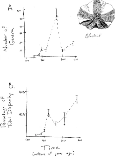
Figure 1.2. Diversity and disparity in the fossil record for the Blastoids. Plots show A. diversity (number of genera) and B. disparity (trait variance) through time. Image by the author, inspired by Foote (1997). This image can be reused under a CC-BY-4.0 license.
phylo-genetic trees do not provide all of the answers. In particular, there are certain problems that comparative data alone simply cannot address. The most promi-nent of these, which I will return to later, are reconstructing traits of particular ancestors (ancestral state reconstruction; Losos 2011) and distinguishing be-tween certain types of models where the tempo of evolution changes through time (Slater et al. 2012a). Some authors have argued that extinction, as well, cannot be detected in the shape of a phylogenetic tree (Rabosky 2010). I will argue against this point of view in Chapter 11, but extinction still remains a tricky problem when one is limited to samples from a single time interval (the present day). Phylogenetic trees provide a rich source of information about the past, but we should be mindful of their limitations (Alroy 1999).
Perhaps the best approach would combine fossil and phylogenetic data directly. Paleontologists studying fossils and neontologists studying phylogenetic trees share a common set of mathematical models. This means that, at some point, the two fields can merge, and both types of information can be combined to study evolutionary patterns in a cohesive and integrative way. However, surprisingly little work has so far been done in this area (but see Slater et al. 2012a, Heath et al. (2014)).
Section 1.5: Overview of the book
In this book, I outline statistical procedures for analyzing comparative data. Some methods – such as those for estimating patterns of speciation and extinc-tion through time – require an ultrametric phylogenetic tree. Other approaches model trait evolution, and thus require data on the traits of species that are included in the phylogenetic tree. The methods also differ as to whether or not they require the phylogenetic tree to be complete – that is, to include every liv-ing species descended from a certain ancestor – or can accommodate a smaller sample of the living species.
The book begins with a general discussion of model-fitting approaches to statis-tics (Chapter 2), with a particular focus on maximum likelihood and Bayesian approaches. In Chapters 3-9, I describe models of character evolution. I discuss approaches to simulating and analyzing the evolution of these characters on a tree. Chapters 10-12 focus on models of diversification, which describe patterns of speciation and extinction through time. I describe methods that allow us to simulate and fit these models to comparative data. Chapter 13 covers com-bined analyses of both character evolution and lineage diversification. Finally, in Chapter 14 I discuss what we have learned so far about evolution from these approaches, and what we are likely to learn in the future.
that this R code will allow further development of this language for compar-ative analyses. However, it is possible to carry out the algorithms we de-scribe using other computer software or programming languages (e.g. Arbor, http://www.arborworkflows.com).
Statistical comparative methods represent a promising future for evolutionary studies, especially as our knowledge of the tree of life expands. I hope that the methods described in this book can serve as a Rosetta stone that will help us read the tree of life as it is being built.
Footnotes
1: This calculation gives the number of distinct tree shapes (ignoring branch lengths) that are fully bifurcating – that is, each species has two descendants -and rooted.
Chapter 2: Fitting Statistical Models to Data
Section 2.1: Introduction
Evolution is the product of a thousand stories. Individual organisms are born, reproduce, and die. The net result of these individual life stories over broad spans of time is evolution. At first glance, it might seem impossible to model this process over more than one or two generations. And yet scientific progress relies on creating simple models and confronting them with data. How can we evaluate models that consider evolution over millions of generations?
There is a solution: we can rely on the properties of large numbers to create simple models that represent, in broad brushstrokes, the types of changes that take place over evolutionary time. We can then compare these models to data in ways that will allow us to gain insights into evolution.
This book is about constructing and testing mathematical models of evolution. In my view the best comparative approaches have two features. First, the most useful methods emphasize parameter estimation over test statistics and P-values. Ideal methods fit models that we care about and estimate parameters that have a clear biological interpretation. To be useful, methods must also recognize and quantify uncertainty in our parameter estimates. Second, many useful methods involve model selection, the process of using data to objectively select the best model from a set of possibilities. When we use a model selection approach, we take advantage of the fact that patterns in empirical data sets will reject some models as implausible and support the predictions of others. This sort of approach can be a nice way to connect the results of a statistical analysis to a particular biological question.
In this chapter, I will first give a brief overview of standard hypothesis testing in the context of phylogenetic comparative methods. However, standard hy-pothesis testing can be limited in complex, real-world situations, such as those encountered commonly in comparative biology. I will then review two other statistical approaches, maximum likelihood and Bayesian analysis, that are of-ten more useful for comparative methods. This latter discussion will cover both parameter estimation and model selection.
All of the basic statistical approaches presented here will be applied to evolution-ary problems in later chapters. It can be hard to understand abstract statistical concepts without examples. So, throughout this part of the chapter, I will refer back to a simple example.
know if this is a fair lizard, where the probability of obtaining heads is 0.5, or not. Perhaps, for example, lizards have a cat-like ability to right themselves when flipped. As an experiment, you flip the lizard 100 times, and obtain heads 63 of those times. Thus, 63 heads out of 100 lizard flips is your data; we will use model comparisons to try to see what these data tell us about models of lizard flipping.
Section 2.2: Standard statistical hypothesis testing
Standard hypothesis testing approaches focus almost entirely on rejecting null hypotheses. In the framework (usually referred to as the frequentist approach to statistics) one first defines a null hypothesis. This null hypothesis represents your expectation if some pattern, such as a difference among groups, is not present, or if some process of interest were not occurring. For example, perhaps you are interested in comparing the mean body size of two species of lizards, an anole and a gecko. Our null hypothesis would be that the two species do not differ in body size. The alternative, which one can conclude by rejecting that null hypothesis, is that one species is larger than the other. Another example might involve investigating two variables, like body size and leg length, across a set of lizard species1. Here the null hypothesis would be that there is no relationship between body size and leg length. The alternative hypothesis, which again represents the situation where the phenomenon of interest is actually occurring, is that there is a relationship with body size and leg length. For frequentist approaches, the alternative hypothesis is always the negation of the null hypothesis; as you will see below, other approaches allow one to compare the fit of a set of models without this restriction and choose the best amongst them.
The next step is to define a test statistic, some way of measuring the patterns in the data. In the two examples above, we would consider test statistics that measure the difference in mean body size among our two species of lizards, or the slope of the relationship between body size and leg length, respectively. One can then compare the value of this test statistic in the data to the expectation of this test statistic under the null hypothesis. The relationship between the test statistic and its expectation under the null hypothesis is captured by a P-value. The P-value is the probability of obtaining a test statistic at least as extreme as the actual test statistic in the case where the null hypothesis is true. You can think of the P-value as a measure of how probable it is that you would obtain your data in a universe where the null hypothesis is true. In other words, the P-value measures how probable it is under the null hypothesis that you would obtain a test statistic at least as extreme as what you see in the data. In particular, if the P-value is very large, sayP = 0.94, then it is extremely likely that your data are compatible with this null hypothesis.
obtain the test statistic seen in the data if the null hypothesis were true. In that case, we reject the null hypothesis as long asP is less than some value chosen in advance. This value is the significance threshold, α, and is almost always set toα= 0.05. By contrast, if that probability is large, then there is nothing “special” about your data, at least from the standpoint of your null hypothesis.
The test statistic is within the range expected under the null hypothesis, and we fail to reject that null hypothesis. Note the careful language here – in a standard frequentist framework, you never accept the null hypothesis, you simply fail to reject it.
Getting back to our lizard-flipping example, we can use a frequentist approach. In this case, our particular example has a name; this is a binomial test, which assesses whether a given event with two outcomes has a certain probability of success. In this case, we are interested in testing the null hypothesis that our lizard is a fair flipper; that is, that the probability of heads pH = 0.5. The binomial test uses the number of “successes” (we will use the number of heads,
H = 63) as a test statistic. We then ask whether this test statistic is either much larger or much smaller than we might expect under our null hypothesis. So, our null hypothesis is thatpH = 0.5; our alternative, then, is thatpH takes some other value: pH ̸= 0.5.
To carry out the test, we first need to consider how many “successes” we should expect if the null hypothesis were true. We consider the distribution of our test statistic (the number of heads) under our null hypothesis (pH = 0.5). This distribution is a binomial distribution (Figure 2.1).
We can use the known probabilities of the binomial distribution to calculate our P-value. We want to know the probability of obtaining a result at least as extreme as our data when drawing from a binomial distribution with parameters
p= 0.5 andn= 100. We calculate the area of this distribution that lies to the right of 63. This area, P = 0.003, can be obtained either from a table, from statistical software, or by using a relatively simple calculation. The value, 0.003, represents the probability of obtaining at least 63 heads out of 100 trials with
pH = 0.5. This number is the P-value from our binomial test. Because we only calculated the area of our null distribution in one tail (in this case, the right, where values are greater than or equal to 63), then this is actually a one-tailed test, and we are only considering part of our null hypothesis wherepH >0.5. Such an approach might be suitable in some cases, but more typically we need to multiply this number by 2 to get a two-tailed test; thus, P = 0.006. This two-tailed P-value of 0.006 includes the possibility of results as extreme as our test statistic in either direction, either too many or too few heads. Since P < 0.05, our chosen αvalue, we reject the null hypothesis, and conclude that we have an unfair lizard.
to each other, there are almost always some differences between them. In fact, for biology, null hypotheses are quite often obviously false. For example, two different species living in different habitats are not identical, and if we measure them enough we will discover this fact. From this point of view, both outcomes of a standard hypothesis test are unenlightening. One either rejects a silly hy-pothesis that was probably known to be false from the start, or one “fails to reject” this null hypothesis2. There is much more information to be gained by estimating parameter values and carrying out model selection in a likelihood or Bayesian framework, as we will see below. Still, frequentist statistical ap-proaches are common, have their place in our toolbox, and will come up in several sections of this book.
One key concept in standard hypothesis testing is the idea of statistical error. Statistical errors come in two flavors: type I and type II errors. Type I errors occur when the null hypothesis is true but the investigator mistakenly rejects it. Standard hypothesis testing controls type I errors using a parameter,α, which defines the accepted rate of type I errors. For example, ifα= 0.05, one should expect to commit a type I error about 5% of the time. When multiple standard hypothesis tests are carried out, investigators often “correct” their P-values using Bonferroni correction. If you do this, then there is only a 5% chance of a single type I error across all of the tests being considered. This singular focus on type I errors, however, has a cost. One can also commit type II errors, when the null hypothesis is false but one fails to reject it. The rate of type II errors in statistical tests can be extremely high. While statisticians do take care to create approaches that have high power, traditional hypothesis testing usually fixes type I errors at 5% while type II error rates remain unknown. There are simple ways to calculate type II error rates (e.g. power analyses) but these are only rarely carried out. Furthermore, Bonferroni correction dramatically increases the type II error rate. This is important because – as stated by Perneger (1998) – “… type II errors are no less false than type I errors.” This extreme emphasis on controlling type I errors at the expense of type II errors is, to me, the main weakness of the frequentist approach3.
I will cover some examples of the frequentist approach in this book, mainly when discussing traditional methods like phylogenetic independent contrasts (PICs). Also, one of the model selection approaches used frequently in this book, likelihood ratio tests, rely on a standard frequentist set-up with null and alternative hypotheses.
and not enough on the size of statistical effects. A small P-value could reflect either a large effect or very large sample sizes or both.
In summary, frequentist statistical methods are common in comparative statis-tics but can be limiting. I will discuss these methods often in this book, mainly due to their prevalent use in the field. At the same time, we will look for alternatives whenever possible.
Section 2.3: Maximum likelihood
Section 2.3a: What is a likelihood?
Since all of the approaches described in the remainer of this chapter involve calculating likelihoods, I will first briefly describe this concept. A good general review of likelihood is Edwards (1992). Likelihood is defined as the probability, given a model and a set of parameter values, of obtaining a particular set of data. That is, given a mathematical description of the world, what is the probability that we would see the actual data that we have collected?
To calculate a likelihood, we have to consider a particular model that may have generated the data. That model will almost always have parameter values that need to be specified. We can refer to this specified model (with particular parameter values) as a hypothesis, H. The likelihood is then:
(eq. 2.1)
L(H|D) =P r(D|H)
Here, L and Pr stand for likelihood and probability, D for the data, and H for the hypothesis, which again includes both the model being considered and a set of parameter values. The | symbol stands for “given,” so equation 2.1 can be read as “the likelihood of the hypothesis given the data is equal to the probability of the data given the hypothesis.” In other words, the likelihood represents the probability under a given model and parameter values that we would obtain the data that we actually see.
For any given model, using different parameter values will generally change the likelihood. As you might guess, we favor parameter values that give us the highest probability of obtaining the data that we see. One way to estimate parameters from data, then, is by finding the parameter values that maximize the likelihood; that is, the parameter values that give the highest likelihood, and the highest probability of obtaining the data. These estimates are then referred to as maximum likelihood (ML) estimates. In an ML framework, we suppose that the hypothesis that has the best fit to the data is the one that has the highest probability of having generated that data.
general, we can write the likelihood for any combination of H “successes” (flips that give heads) out of n trials. We will also have one parameter,pH, which will represent the probability of “success,” that is, the probability that any one flip comes up heads. We can calculate the likelihood of our data using the binomial theorem:
(eq. 2.2)
L(H|D) =P r(D|p) = (
n H
)
pHH(1−pH)n−H
In the example given, n = 100 and H = 63, so: (eq. 2.3)
L(H|D) = (
100 63
)
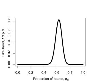
[image:20.612.144.448.307.590.2]p63H(1−pH)37
We can make a plot of the likelihood,L, as a function ofpH (Figure 2.2). When we do this, we see that the maximum likelihood value ofpH, which we can call
ˆ
pH, is atpˆH = 0.63. This is the “brute force” approach to finding the maximum likelihood: try many different values of the parameters and pick the one with the highest likelihood. We can do this much more efficiently using numerical methods as described in later chapters in this book.
We could also have obtained the maximum likelihood estimate for pH through differentiation. This problem is much easier if we work with the ln-likelihood rather than the likelihood itself (note that whatever value ofpH that maximizes the likelihood will also maximize the ln-likelihood, because the log function is strictly increasing). So:
(eq. 2.4)
lnL= ln (
n H
)
+HlnpH+ (n−H) ln (1−pH)
Note that the natural log (ln) transformation changes our equation from a power function to a linear function that is easy to solve. We can differentiate: (eq. 2.5)
dlnL dpH
= H
pH
− (n−H)
(1−pH)
The maximum of the likelihood represents a peak, which we can find by setting the derivative dlnL
dpH to zero. We then find the value of pH that solves that equation, which will be our estimatepˆH. So we have:
(eq. 2.6)
H ˆ pH −
n−H
1−pˆH = 0 H
ˆ
pH =
n−H 1−pˆH
H(1−pˆH) = pˆH(n−H)
H−HpˆH = npˆH−HpˆH
H = npˆH
ˆ
pH = H/n
Notice that, for our simple example, H/n = 63/100 = 0.63, which is exactly equal to the maximum likelihood from figure 2.2.
Maximum likelihood estimates have many desirable statistical properties. It is worth noting, however, that they will not always return accurate parameter estimates, even when the data is generated under the actual model we are considering. In fact, ML parameters can sometimes be biased. To understand what this means, we need to formally introduce two new concepts: bias and precision. Imagine that we were to simulate datasets under some model A with parameter a. For each simulation, we then used ML to estimate the parameteraˆ
how close our estimatesˆaiare to the true valuea. If our ML parameter estimate is biased, then the average of theaˆi will differ from the true valuea. It is not uncommon for ML estimates to be biased in a way that depends on sample size, so that the estimates get closer to the truth as sample size increases, but can be quite far off in a particular direction when the number of data points is small compared to the number of parameters being estimated.
In our example of lizard flipping, we estimated a parameter value ofpˆH = 0.63. For the particular case of estimating the parameter of a binomial distribution, our ML estimate is known to be unbiased. And this estimate is different from 0.5 – which was our expectation under the null hypothesis. So is this lizard fair? Or, alternatively, can we reject the null hypothesis thatpH = 0.5? To evaluate this, we need to use model selection.
Section 2.3b: The likelihood ratio test
Model selection involves comparing a set of potential models and using some criterion to select the one that provides the “best” explanation of the data. Different approaches define “best” in different ways. I will first discuss the simplest, but also the most limited, of these techniques, the likelihood ratio test. Likelihood ratio tests can only be used in one particular situation: to compare two models where one of the models is a special case of the other. This means that model A is exactly equivalent to the more complex model B with parameters restricted to certain values. We can always identify the simpler model as the model with fewer parameters. For example, perhaps model B has parameters x, y, and z that can take on any values. Model A is the same as model B but with parameter z fixed at 0. That is, A is the special case of B when parameter z = 0. This is sometimes described as model A is nested within model B, since every possible version of model A is equal to a certain case of model B, but model B also includes more possibilities.
For likelihood ratio tests, the null hypothesis is always the simpler of the two models. We compare the data to what we would expect if the simpler (null) model were correct.
For example, consider again our example of flipping a lizard. One model is that the lizard is “fair:” that is, that the probability of heads is equal to 1/2. A different model might be that the probability of heads is some other value p, which could be 1/2, 1/3, or any other value between 0 and 1. Here, the latter (complex) model has one additional parameter, pH, compared to the former (simple) model; the simple model is a special case of the complex model when
pH = 1/2.
For such nested models, one can calculate the likelihood ratio test statistic as (eq. 2.7)
∆ = 2·lnL1
L2
Here, ∆ is the likelihood ratio test statistic, L2 the likelihood of the more complex (parameter rich) model, and L1 the likelihood of the simpler model. Since the models are nested, the likelihood of the complex model will always be greater than or equal to the likelihood of the simple model. This is a direct consequence of the fact that the models are nested. If we find a particular likelihood for the simpler model, we can always find a likelihood equal to that for the complex model by setting the parameters so that the complex model is equivalent to the simple model. So the maximum likelihood for the complex model will either be that value, or some higher value that we can find through searching the parameter space. This means that the test statistic∆ will never be negative. In fact, if you ever obtain a negative likelihood ratio test statistic, something has gone wrong – either your calculations are wrong, or you have not actually found ML solutions, or the models are not actually nested.
To carry out a statistical test comparing the two models, we compare the test statistic ∆ to its expectation under the null hypothesis. When sample sizes are large, the null distribution of the likelihood ratio test statistic follows a chi-squared (χ2) distribution with degrees of freedom equal to the difference in the number of parameters between the two models. This means that if the simpler hypothesis were true, and one carried out this test many times on large independent datasets, the test statistic would approximately follow this
χ2distribution. To reject the simpler (null) model, then, one compares the test statistic with a critical value derived from the appropriateχ2 distribution. If the test statistic is larger than the critical value, one rejects the null hypothesis. Otherwise, we fail to reject the null hypothesis. In this case, we only need to consider one tail of theχ2test, as every deviation from the null model will push us towards higher∆ values and towards the right tail of the distribution. For the lizard flip example above, we can calculate the ln-likelihood under a hypothesis ofpH= 0.5as:
(eq. 2.8)
lnL1 = ln
(100
63
)
+ 63·ln 0.5 + (100−63)·ln (1−0.5) lnL1 = −5.92
We can compare this to the likelihood of our maximum-likelihood estimate : (eq. 2.9)
lnL2 = ln
(100
63
)
+ 63·ln 0.63 + (100−63)·ln (1−0.63) lnL2 = −2.50
(eq. 2.10)
∆ = 2·(lnL2−lnL1)
∆ = 2·(−2.50− −5.92) ∆ = 6.84
If we compare this to a χ2 distribution with one d.f., we find that P = 0.009. Because this P-value is less than the threshold of 0.05, we reject the null hy-pothesis, and support the alternative. We conclude that this is not a fair lizard. As you might expect, this result is consistent with our answer from the bino-mial test in the previous section. However, the approaches are mathematically different, so the two P-values are not identical.
Although described above in terms of two competing hypotheses, likelihood ratio tests can be applied to more complex situations with more than two competing models. For example, if all of the models form a sequence of increasing com-plexity, with each model a special case of the next more complex model, one can compare each pair of hypotheses in sequence, stopping the first time the test statistic is non-significant. Alternatively, in some cases, hypotheses can be placed in a bifurcating choice tree, and one can proceed from simple to complex models down a particular path of paired comparisons of nested models. This approach is commonly used to select models of DNA sequence evolution (Posada and Crandall 1998).
Section 2.3c: The Akaike information criterion (AIC)
You might have noticed that the likelihood ratio test described above has some limitations. Especially for models involving more than one parameter, ap-proaches based on likelihood ratio tests can only do so much. For example, one can compare a series of models, some of which are nested within others, using an ordered series of likelihood ratio tests. However, results will often de-pend strongly on the order in which tests are carried out. Furthermore, often we want to compare models that are not nested, as required by likelihood ratio tests. For these reasons, another approach, based on the Akaike Information Criterion (AIC), can be useful.
The AIC value for a particular model is a simple function of the likelihood L and the number of parameters k:
(eq. 2.11)
AIC= 2k−2lnL
description of AIC does not capture the actual mathematical and philosoph-ical justification for equation (2.11). In fact, this equation is not arbitrary; instead, its exact trade-off between parameter numbers and log-likelihood dif-ference comes from information theory (for more information, see Burnham and Anderson 2003, Akaike (1998)).
The AIC equation (2.11) above is only valid for quite large sample sizes relative to the number of parameters being estimated (for n samples and k parameters,
n/k >40). Most empirical data sets include fewer than 40 independent data points per parameter, so a small sample size correction should be employed: (eq. 2.12)
AICC =AIC+
2k(k+ 1)
n−k−1
This correction penalizes models that have small sample sizes relative to the number of parameters; that is, models where there are nearly as many parame-ters as data points. As noted by Burnham and Anderson (2003), this correction has little effect if sample sizes are large, and so provides a robust way to correct for possible bias in data sets of any size. I recommend always using the small sample size correction when calculating AIC values.
To select among models, one can then compare their AICc scores, and choose the model with the smallest value. It is easier to make comparisons in AICc scores between models by calculating the difference, ∆AICc. For example, if you are comparing a set of models, you can calculate ∆AICc for model i as: (eq. 2.13)
∆AICci =AICci−AICcmin
whereAICci is theAICc score for model i andAICcmin is the minimum AICc score across all of the models.
As a broad rule of thumb for comparingAICvalues, any model with a∆AICci of less than four is roughly equivalent to the model with the lowestAICcvalue. Models with∆AICci between 4 and 8 have little support in the data, while any model with a∆AICci greater than 10 can safely be ignored.
Additionally, one can calculate the relative support for each model using Akaike weights. The weight for model i compared to a set of competing models is calculated as:
(eq. 2.14)
wi =
e−∆AICci/2
∑
ie−
∆AICci/2
Returning to our example of lizard flipping, we can calculate AICc scores for our two models as follows:
(eq. 2.15)
AIC1 = 2k1−2lnL1= 2·0−2· −5.92
AIC1 = 11.8
AIC2 = 2k2−2lnL2= 2·1−2· −2.50
AIC2 = 7.0
Our example is a bit unusual in that model one has no estimated parameters; this happens sometimes but is not typical for biological applications. We can correct these values for our sample size, which in this case is n = 100 lizard flips:
(eq. 2.16)
AICc1 = AIC1+
2k1(k1+1)
n−k1−1
AICc1 = 11.8 +
2·0(0+1) 100−0−1
AICc1 = 11.8
AICc2 = AIC2+
2k2(k2+1)
n−k2−1
AICc2 = 7.0 +
2·1(1+1) 100−1−1
AICc2 = 7.0
Notice that, in this particular case, the correction did not affect ourAICvalues, at least to one decimal place. This is because the sample size is large relative to the number of parameters. Note that model 2 has the smallestAICc score and is thus the model that is best supported by the data. Noting this, we can now convert theseAICc scores to a relative scale:
(eq. 2.17)
∆AICc1 = AICc1−AICcmin
= 11.8−7.0 = 4.8
∆AICc2 = AICc2−AICcmin
= 7.0−7.0
= 0
and the likelihood ratio test. Finally, we can use the relative AICc scores to calculate Akaike weights:
(eq. 2.18)
∑
ie−
∆i/2 = e−∆1/2+e−∆2/2
= e−4.8/2+e−0/2
= 0.09 + 1 = 1.09
w1 = e
−∆AICc1/2
∑
ie
−∆AICci /2
= 0.091.09 = 0.08
w2 = e
−∆AICc2/2
∑
ie
−∆AICci /2
= 1.001.09 = 0.92
Our results are again consistent with the results of the likelihood ratio test. The relative likelihood of an unfair lizard is 0.92, and we can be quite confident that our lizard is not a fair flipper.
AIC weights are also useful for another purpose: we can use them to get model-averaged parameter estimates. These are parameter estimates that are com-bined across different models proportional to the support for those models. As a thought example, imagine that we are considering two models, A and B, for a particular dataset. Both model A and model B have the same parameter p, and this is the parameter we are particularly interested in. In other words, we do not know which model is the best model for our data, but what we really need is a good estimate ofp. We can do that using model averaging. If model A has a high AIC weight, then the model-averaged parameter estimate for p
Section 2.4: Bayesian statistics
Section 2.4a: Bayes Theorem
Recent years have seen tremendous growth of Bayesian approaches in recon-structing phylogenetic trees and estimating their branch lengths. Although there are currently only a few Bayesian comparative methods, their number will certainly grow as comparative biologists try to solve more complex problems. In a Bayesian framework, the quantity of interest is the posterior probability, calculated using Bayes’ theorem:
(eq. 2.19)
P r(H|D) = P r(D|H)·P r(H)
P r(D)
The benefit of Bayesian approaches is that they allow us to estimate the prob-ability that the hypothesis is true given the observed data, P r(H|D). This is really the sort of probability that most people have in mind when they are thinking about the goals of their study. However, Bayes theorem also reveals a cost of this approach. Along with the likelihood, P r(D|H), one must also incorporate prior knowledge about the probability that any given hypothesis is true - P r(H). This represents the prior belief that a hypothesis is true, even before consideration of the data at hand. This prior probability must be explic-itly quantified in all Bayesian statistical analyses. In practice, scientists often seek to use “uninformative” priors that have little influence on the posterior dis-tribution - although even the term “uninformative” can be confusing, because the prior is an integral part of a Bayesian analysis. The termP r(D)is also an important part of Bayes theorem, and can be calculated as the probability of obtaining the data integrated over the prior distributions of the parameters: (eq. 2.20)
P r(D) = ∫
H
P r(H|D)P r(H)dH
However, P r(D) is constant when comparing the fit of different models for a given data set and thus has no influence on Bayesian model selection under most circumstances (and all the examples in this book).
In our example of lizard flipping, we can do an analysis in a Bayesian framework. For model 1, there are no free parameters. Because of this, P r(H) = 1 and
If we consider model 2 above, the parameterpH must be estimated. We can set a uniform prior between 0 and 1 forpH, so thatf(pH) = 1for all pH in the interval [0,1]. We can also write this as “our prior forph is U(0,1)”. Then: (eq. 2.21)
P r(H|D) =P r(D|H)·P r(H)
P r(D) =
P(H|pH, N)f(pH)
∫1
0 P(H|pH, N)f(ph)dpH
Next we note thatP r(D|H)is the likelihood of our data given the model, which is already stated above as equation 2.2. Plugging this into our equation, we have: (eq. 2.22)
P r(H|D) = (N
H
)
pHH(1−pH)N−H
∫1 0 (N H ) pH
H(1−pH)N−HdpH
This ugly equation actually simplifies to a beta distribution, which can be ex-pressed more simply as:
(eq. 2.23)
P r(H|D) = (N+ 1)!
H!(N−H)!p
H
H(1−pH)N−H
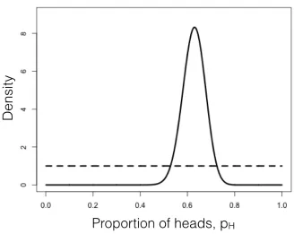
We can compare this posterior distribution of our parameter estimate,pH, given the data, to our uniform prior (Figure 2.3). If you inspect this plot, you see that the posterior distribution is very different from the prior – that is, the data have changed our view of the values that parameters should take. Again, this result is qualitatively consistent with both the frequentist and ML approaches described above. In this case, we can see from the posterior distribution that we can be quite confident that our parameterpH is not 0.5.
As you can see from this example, Bayes theorem lets us combine our prior belief about parameter values with the information from the data in order to obtain a posterior. These posterior distributions are very easy to interpret, as they express the probability of the model parameters given our data. However, that clarity comes at a cost of requiring an explicit prior. Later in the book we will learn how to use this feature of Bayesian statistics to our advantage when we actually do have some prior knowledge about parameter values.
Section 2.4b: Bayesian MCMC
but not complicated mathematics (e.g. integration of probability distributions, as in equation 2.22), and so represents a more flexible approach to Bayesian computation. Frequently, the integrals in equation 2.21 are intractable, so that the most efficient way to fit Bayesian models is by using MCMC. Also, setting up an MCMC is, in my experience, easier than people expect!
An MCMC analysis requires that one constructs and samples from a Markov chain. A Markov chain is a random process that changes from one state to another with certain probabilities that depend only on the current state of the system, and not what has come before. A simple example of a Markov chain is the movement of a playing piece in the game Chutes and Ladders; the position of the piece moves from one square to another following probabilities given by the dice and the layout of the game board. The movement of the piece from any square on the board does not depend on how the piece got to that square. Some Markov chains have an equilibrium distribution, which is a stable probabil-ity distribution of the model’s states after the chain has run for a very long time. For Bayesian analysis, we use a technique called a Metropolis-Hasting algorithm to construct a special Markov chain that has an equilibrium distribution that is the same as the Bayesian posterior distribution of our statistical model. Then, using a random simulation on this chain (this is the Markov-chain Monte Carlo, MCMC), we can sample from the posterior distribution of our model.
In simpler terms: we use a set of well-defined rules. These rules let us walk around parameter space, at each step deciding whether to accept or reject the next proposed move. Because of some mathematical proofs that are beyond the scope of this chapter, these rules guarantee that we will eventually be accepting samples from the Bayesian posterior distribution - which is what we seek. The following algorithm uses a Metropolis-Hastings algorithm to carry out a Bayesian MCMC analysis with one free parameter:
1. Get a starting parameter value.
• Sample a starting parameter value,p0, from the prior distribution. 2. Starting withi= 1, propose a new parameter for generation i.
• Given the current parameter value,p, select a new proposed param-eter value,p′, using the proposal densityQ(p′|p).
3. Calculate three ratios.
• a. The prior odds ratio. This is the ratio of the probability of drawing the parameter valuespandp′from the prior (eq. 2.24).
Rprior=
P(p′)
P(p)
Q(p′|p) =Q(p|p′)anda2= 1, simplifying the calculations (eq. 2.25).
Rproposal=
Q(p′|p)
Q(p|p′)
• c. The likelihood ratio. This is the ratio of probabilities of the data given the two different parameter values (eq. 2.26).
Rlikelihood =
L(p′|D)
L(p|D) =
P(D|p′)
P(D|p)
4. Multiply. Find the product of the prior odds, proposal density ratio, and the likelihood ratio (eq. 2.27).
Raccept=Rprior·Rproposal·Rlikelihood
5. Accept or reject. Draw a random numberxfrom a uniform distribution between 0 and 1. Ifx < Raccept, accept the proposed value ofp′(pi=p′); otherwise reject, and retain the current valuep(pi=p).
6. Repeat. Repeat steps 2-5 a large number of times.
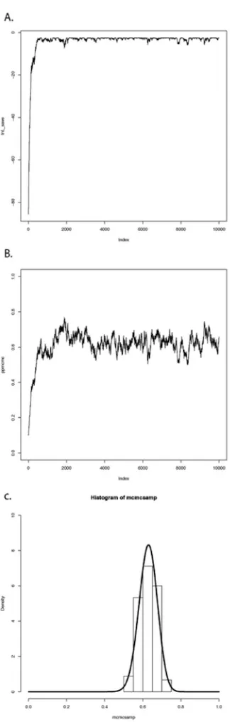
Carrying out these steps, one obtains a set of parameter values,pi, wherei is from 1 to the total number of generations in the MCMC. Typically, the chain has a “burn-in” period at the beginning. This is the time before the chain has reached a stationary distribution, and can be observed when parameter values show trends through time and the likelihood for models has yet to plateau. If you eliminate this “burn-in” period, then, as discussed above, each step in the chain is a sample from the posterior distribution. We can summarize the posterior distributions of the model parameters in a variety of ways; for example, by calculating means, 95% confidence intervals, or histograms.
We can apply this algorithm to our coin-flipping example. We will consider the same prior distribution, U(0,1), for the parameterp. We will also define a proposal density,Q(p′|p)U(p−ϵ, p+ϵ). That is, we will add or subtract a small number (ϵ≤0.01) to generate proposed values ofp′givenp.
To start the algorithm, we draw a value of p from the prior. Let’s say for illustrative purposes that the value we draw is 0.60. This becomes our current parameter estimate. For step two, we propose a new value,p′, by drawing from
our proposal distribution. We can use ϵ = 0.01 so the proposal distribution becomesU(0.59,0.61). Let’s suppose that our new proposed valuep′= 0.595. We then calculate our three ratios. Here things are simpler than you might have expected for two reasons. First, recall that our prior probability distribution is
U(0,1). The density of this distribution is a constant (1.0) for all values of p
(eq. 2.28)
Rprior=
P(p′)
P(p) = 1 1 = 1
Similarly, because our proposal distribution is symmetrical, Q(p′|p) = Q(p|p′)
and Rproposal = 1. That means that we only need to calculate the likelihood ratio,Rlikelihood forpand p′. We can do this by plugging our values forp(or
p′) into equation 2.2: (eq. 2.29)
P(D|p) = (
N H
)
pH(1−p)N−H = (
100 63
)
0.663(1−0.6)100−63= 0.068
Likewise, (eq. 2.30)
P(D|p′) = (
N H
)
p′H(1−p′)N−H = (
100 63
)
0.59563(1−0.595)100−63= 0.064
The likelihood ratio is then: (eq. 2.31)
Rlikelihood =
P(D|p′)
P(D|p) = 0.064 0.068 = 0.94
We can now calculateRaccept=Rprior·Rproposal·Rlikelihood= 1·1·0.94 = 0.94. We next choose a random number between 0 and 1 – say that we drawx= 0.34. We then notice that our random numberxis less than or equal to Raccept, so we accept the proposed value ofp′. If the random number that we drew were greater than 0.94, we would reject the proposed value, and keep our original parameter valuep= 0.60going into the next generation.
general, analytic posterior distributions are difficult or impossible to construct, so approximation using MCMC is very common.
This simple example glosses over some of the details of MCMC algorithms, but we will get into those details later, and there are many other books that treat this topic in great depth (e.g. Christensen et al. 2010). The point is that we can solve some of the challenges involved in Bayesian statistics using numerical “tricks” like MCMC, that exploit the power of modern computers to fit models
and estimate model parameters.
Section 2.4c: Bayes factors
Now that we know how to use data and a prior to calculate a posterior dis-tribution, we can move to the topic of Bayesian model selection. We already learned one general method for model selection using AIC. We can also do model selection in a Bayesian framework. The simplest way is to calculate and then compare the posterior probabilities for a set of models under consideration. One can do this by calculating Bayes factors:
(eq. 2.32)
B12=
P r(D|H1)
P r(D|H2)
Bayes factors are ratios of the marginal likelihoods P(D|H)of two competing models. They represent the probability of the data averaged over the posterior distribution of parameter estimates. It is important to note that these marginal likelihoods are different from the likelihoods used above forAICmodel compar-ison in an important way. WithAIC and other related tests, we calculate the likelihoods for a given model and a particular set of parameter values – in the coin flipping example, the likelihood for model 2 whenpH = 0.63. By contrast, Bayes factors’ marginal likelihoods give the probability of the data averaged over all possible parameter values for a model, weighted by their prior probability. Because of the use of marginal likelihoods, Bayes factor allows us to do model selection in a way that accounts for uncertainty in our parameter estimates – again, though, at the cost of requiring explicit prior probabilities for all model parameters. Such comparisons can be quite different from likelihood ratio tests or comparisons ofAICc scores. Bayes factors represent model comparisons that integrate over all possible parameter values rather than comparing the fit of models only at the parameter values that best fit the data. In other words,
Calculation of Bayes factors can be quite complicated, requiring integration across probability distributions. In the case of our coin-flipping problem, we have already done that to obtain the beta distribution in equation 2.22. We can then calculate Bayes factors to compare the fit of two competing models. Let’s compare the two models for coin flipping considered above: model 1, where
pH = 0.5, and model 2, wherepH = 0.63. Then: (eq. 2.33)
P r(D|H1) =
(100
63
)
0.50.63(1−0.5)100−63
= 0.00270
P r(D|H2) =
∫1 p=0
(100 63
)
p63(1−p)100−63 = (10063)β(38,64)
= 0.0099
B12 = 0.002700.0099
= 3.67
In the above example,β(x, y)is the Beta function. Our calculations show that the Bayes factor is 3.67 in favor of model 2 compared to model 1. This is typically interpreted as substantial (but not decisive) evidence in favor of model 2. Again, we can be reasonably confident that our lizard is not a fair flipper. In the lizard flipping example we can calculate Bayes factors exactly because we know the solution to the integral in equation 2.33. However, if we don’t know how to solve this equation (a typical situation in comparative methods), we can still approximate Bayes factors from our MCMC runs. Methods to do this, including arrogance sampling and stepping stone models (Xie et al. 2011; Perrakis et al. 2014), are complex and beyond the scope of this book. However, one common method for approximating Bayes Factors involves calculating the harmonic mean of the likelihoods over the MCMC chain for each model. The ratio of these two likelihoods is then used as an approximation of the Bayes factor (Newton and Raftery 1994). Unfortunately, this method is extremely unreliable, and probably should never be used (see Neal 2008 for more details).
Section 2.5: AIC versus Bayes
identify the model that most efficiently captures the information in your data. That is, even though both techniques are carrying out model selection, the basic philosophy of how these models are being considered is very different: choosing the best of several simplified models of reality, or choosing the correct model from a set of alternatives.
The debate between Bayesian and likelihood-based approaches often centers around the use of priors in Bayesian statistics, but the distinction between models and “reality” is also important. More specifically, it is hard to imagine a case in comparative biology where one would be justified in the Bayesian assumption that one has identified the true model that generated the data. This also explains whyAIC-based approaches typically select more complex models than Bayesian approaches. In anAIC framework, one assumes that reality is very complex and that models are approximations; the goal is to figure out how much added model complexity is required to efficiently explain the data. In cases where the data are actually generated under a very simple model, AIC
may err in favor of overly complex models. By contrast, Bayesian analyses assume that one of the models being considered is correct. This type of analysis will typically behave appropriately when the data are generated under a simple model, but may be unpredictable when data are generated by processes that are not considered by any of the models. However, Bayesian methods account for uncertainty much better than AIC methods, and uncertainty is a fundamental aspect of phylogenetic comparative methods.
In summary, Bayesian approaches are useful tools for comparative biology, es-pecially when combined with MCMC computational techniques. They require specification of a prior distribution and assume that the “true” model is among those being considered, both of which can be drawbacks in some situations. A Bayesian framework also allows us to much more easily account for phylo-genetic uncertainty in comparative analysis. Many comparative biologists are pragmatic, and use whatever methods are available to analyze their data. This is a reasonable approach but one should remember the assumptions that underlie any statistical result.
Section 2.6: Models and comparative methods
it is extendable; one can create new models and automatically fit them into a preexisting framework for data analysis. Finally, it is powerful; a model fitting approach allows us to construct comparative tests that relate directly to particular biological hypotheses.
Footnotes
1: I assume here that you have little interest in organisms other than lizards. 2: And, often, concludes that we just “need more data” to get the answer that we want.
Chapter 3: Introduction to Brownian Motion
Section 3.1: Introduction
Squamates, the group that includes snakes and lizards, is exceptionally diverse. Since sharing a common ancestor between 150 and 210 million years ago (Hedges and Kumar 2009), squamates have diversified to include species that are very large and very small; herbivores and carnivores; species with legs and species that are legless. How did that diversity of species’ traits evolve? How did these characters first come to be, and how rapidly did they change to explain the diversity that we see on earth today? In this chapter, we will begin to discuss models for the evolution of species’ traits.
Imagine that you want to use statistical approaches to understand how traits change through time. To do that, you need to have an exact mathematical specification of how evolution takes place. Obviously there are a wide variety of models of trait evolution, from simple to complex. For example, you might create a model where a trait starts with a certain value and has some constant probability of changing in any unit of time. Alternatively, you might make a model that is more detailed and explicit, and considers a large set of individuals in a population. You could assign genotypes to each individual and allow the population to evolve through reproduction and natural selection.
In this chapter – and in comparative methods as a whole – the models we will consider will be much closer to the first of these two models. However, there are still important connections between these simple models and more realistic models of trait evolution (see chapter five).
In the next six chapters, I will discuss models for two different types of characters. In this chapter and chapters four, five, and six, I will consider traits that follow continuous distributions – that is, traits that can have real-numbered values. For example, body mass in kilograms is a continuous character. I will discuss the most commonly used model for these continuous characters, Brownian motion, in this chapter and the next, while chapter five covers analyses of multivariate Brownian motion. We will go beyond Brownian motion in chapter six. In chapter seven and the chapters that immediately follow, I will cover discrete characters, characters that can occupy one of a number of distinct character states (for example, species of squamates can either be legless or have legs).
Section 3.2: Properties of Brownian Motion
a bit hard to picture, but the logic applies equally well to the movement of a large ball over a crowd in a stadium. When the ball is over the crowd, people push on it from many directions. The sum of these many small forces determine the movement of the ball. Again, the movement of the ball can be modeled using Brownian motion1.
The core idea of this example is that the motion of the object is due to the sum of a large number of very small, random forces. This idea is a key part of biological models of evolution under Brownian motion. It is worth mentioning that even though Brownian motion involves change that has a strong random component, it is incorrect to equate Brownian motion models with models of pure genetic drift (as explained in more detail below).
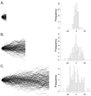
Brownian motion is a popular model in comparative biology because it captures the way traits might evolve under a reasonably wide range of scenarios. However, perhaps the main reason for the dominance of Brownian motion as a model is that it has some very convenient statistical properties that allow relatively simple analyses and calculations on trees. I will use some simple simulations to show how the Brownian motion model behaves. I will then list the three critical statistical properties of Brownian motion, and explain how we can use these properties to apply Brownian motion models to phylogenetic comparative trees. When we model evolution using Brownian motion, we are typically discussing the dynamics of the mean character value, which we will denote as¯z, in a pop-ulation. That is, we imagine that you can measure a sample of the individuals in a population and estimate the mean average trait value. We will denote the mean trait value at some timet as z¯(t). We can model the mean trait value through time with a Brownian motion process.
Brownian motion models can be completely described by two parameters. The first is the starting value of the population mean trait,z¯(0). This is the mean trait value that is seen in the ancestral population at the start of the simulation, before any trait change occurs. The second parameter of Brownian motion is the evolutionary rate parameter,σ2. This parameter determines how fast traits will randomly walk through time.
At the core of Brownian motion is the normal distribution. You might know that a normal distribution can be described by two parameters, the mean and variance. Under Brownian motion, changes in trait values over any interval of time are always drawn from a normal distribution with mean 0 and variance proportional to the product of the rate of evolution and the length of time (variance =σ2t). As I will show later, we can simulate change under Brownian motion model by drawing from normal distributions. Another way to say this more simply is that we can always describe how much change to expect under Brownian motion using normal distributions. These normal distributions for expected changes have a mean of zero and get wider as the time interval we consider gets longer.