Signal Computing: Digital Signals in the Software Domain

(1)

Signal Computing:

Digital Signals in the Software Domain

Fall 2016

Michael Stiber Bilin Zhang Stiber

University of Washington Bothell 18115 Campus Way NE

Bothell, Washington 98011

Eric C. Larson

Southern Methodist University Lyle School of Engineering 3145 Dyer Street

(2)

Copyright c2002–2016 by Michael and Bilin Stiber and Eric C. Larson

This material is based upon work supported by the National Science Foundation under Grant No. 0443118.

This work is licensed under the Creative Commons Attribution-ShareAlike 4.0 International License. To view a copy of this license, visit

(3)

List of Figures

0.1 Course conceptual road map . . . xv

1.1 Schematic diagram of a CRT. . . 4

1.2 Interlaced and non-interlaced raster scanning . . . 5

1.3 Real periodic signals . . . 7

1.4 Components of a phasor are sinusoids. . . 9

1.5 Graphical summation of vectors.. . . 10

1.6 Phasor representation of beating. . . 13

1.7 Amplitude vs. time representation of beating. . . 13

1.8 A train of periodic rectangular pulses . . . 21

1.9 The sinc function. . . 22

1.10 First 12 terms in the Fourier series for a periodic sequence of rectangular pulses 24 1.11 First 100 terms in the Fourier series for a periodic sequence of rectangular pulses 25 1.12 Spectrum of a periodic sequence of rectangular pulses . . . 26

1.13 Spectrum of a periodic sequence of rectangular pulses; varying pulse width . 27 1.14 Spectrum of a periodic sequence of rectangular pulses; varying period . . . . 28

2.1 Block diagram of the data acquisition process. . . 31

2.2 Sample and hold output . . . 34

2.3 Sampling and apparent frequency . . . 35

2.4 Error in output for 8-bit ADC . . . 39

3.1 Four frequency components . . . 46

3.2 Filter frequency response . . . 47

3.3 A filtered signal . . . 47

3.4 Unfiltered vs. filtered signal . . . 48

3.5 A basic feedforward filter block diagram. . . 48

3.6 Treat transfer function as a black box. . . 55

3.7 Two zero filterr = 0.9, ˆω0 =±π/2. . . 58

3.8 Two zero filterr = 0.9, ˆω0 =±5π/6. . . 58

(8)

LIST OF FIGURES

3.10 Two sinusoid spectrum . . . 64

4.1 The exponential signal x[n] = (1/2)n, n= 0,1,2, . . .. . . 71

4.2 Frequency content of the signal shown in figure 4.1. . . 72

4.3 Frequency content of the unit step signal. . . 73

4.4 Example of convolution function execution for nx = 5 and nh = 2. . . 77

4.5 Convolution of en_∗en . . . 78

5.1 Block diagram of a simple filter with both feedforward and feedback terms. . 85

5.2 One pole in the z-plane, located at r= 0.9 and ˆω0 =π/2. . . 87

5.3 Magnitude response of two filters . . . 87

5.4 Block diagram of a filter with M feedforward and N feedback terms. . . 90

5.5 One polea1 =rejωˆ0 in z-plane. r =R, ˆω0 = 0 and z =ejωˆ . . . 92

5.6 Feedback filter design . . . 94

5.7 Example filter frequency responses . . . 96

6.1 A rectangular pulse with widthτ. . . 102

6.2 Fourier transform of the pulse in figure 6.1. . . 103

6.3 Fourier transform of a rectangular pulse for various width values . . . 104

6.4 Plot of the sequence x[n] = 0.8n _{and the magnitude of its DFT} _{. . . 110}

6.5 First half of DFT of x[n] = 0.8n _{. . . 111}

6.6 Schematic outline of an iterative 8-point FFT . . . 116

6.7 Sum of two sinusoids with 512 samples and its FFT . . . 119

6.8 Sum of two sinusoids with 512 samples and its FFT; different frequencies . . 120

6.9 Magnitude spectrum of windowed signalx[n] = cos ˆω0n . . . 122

6.10 Magnitude spectrum of a one-sided signal x[n] = cos ˆω0n with ˆω0 = 0.2π. . . 123

6.11 Magnitude spectrum of the signal (6-55) made up of three sinusoids . . . 125

6.12 The same figure as 6.11, but with rectangular window length N = 128 . . . . 125

6.13 Bird call waveform and spectrogram; window size 512 samples, overlap 511 . 127 6.14 Bird call waveform and spectrogram; window size 128 samples, overlap 127 . 127 6.15 Different bird call waveform and spectrogram; 512 sample window, overlap 511129 6.16 Bird call waveform; 128 sample window, overlap 127 . . . 129

6.17 A 512-point Hann window in the time domain. . . 130

6.18 The 512-point Bartlett window in the time domain. . . 130

6.19 Hann windowed cosine waveform and its spectrum . . . 131

6.20 Bartlett windowed cosine waveform and its spectrum . . . 132

6.21 Comparison between Hann and Bartlett windows for a cosine wave . . . 133

6.22 Similar spectrogram as figure 6.14, but here a rectangular window is used. . 133

6.23 Similar spectrogram as figure 6.16, but here a rectangular window is used. . 134

7.1 Shannon’s model for coding information for transmission. . . 138

7.2 A taxonomy of coding/compression schemes. . . 140

7.3 Generalized scheme for encoding. . . 140

(9)

LIST OF FIGURES

8.1 Block diagram of JPEG encoder and decoder. . . 154

8.2 Illustration of transform of 8x8 pixel block into 8x8 spectrum by DCT . . . . 155

8.3 Example 2D spectra . . . 156

8.4 Example spectrum (right) of an 8x8 block taken from a natural image. . . . 157

8.5 Entropy coding of JPEG DCT blocks . . . 158

8.6 Simplified block diagram of an MPEG video source encoder . . . 159

9.1 Block diagram of a generic multimedia system. . . 164

9.2 Simplified block diagram of a CD player. . . 168

(10)

(11)

List of Tables

4.1 Summary of frequency transforms. . . 68

4.2 Some properties of the z-transform. . . 79

6.1 Some examples of how ∆ˆω, ∆ω = ∆ˆωfs, and ∆f = ∆ω/2π = fs/N change for signals of different duration and sampling rate. . . 106

6.2 Example of the effect of bit reversal on an eight-element input vector. . . 114

7.1 Two binary codes. . . 143

(12)

(13)

List of Algorithms

3.1 Generate two sinusoids. . . 63

3.2 Filtering.. . . 63

4.1 Discrete convolution. . . 76

6.1 Recursive FFT. . . 114

(14)

(15)

Preface

As computers become ubiquitous, they become more and more embedded not only in the devices we own and use but in our lives. As a result, computers become embedded in the physical world, with their primary purpose being to detect and analyze happenings in our world and to produce responses that affect that world. As computing professionals, we need to understand how computers can process information from the physical world asdigital signals: multimedia (sound, images, video) and other measurements (in medical instruments, cars, cell phones, eyeglasses, etc). This is why we have chosen to coin the phrase “Signal Computing”.

Digital signals place great demands on processing power, network bandwidth, storage capacity, I/O speed, and software design. As a result, signal computing is a great laboratory for exercising the full range of knowledge of computer science.

In this book, you will learn how digital signals are captured, represented, processed, communicated, and stored in computers. The specific topics we will cover include: physical properties of the source information (such as sound or images), devices for information cap-ture (microphones, cameras), digitization, compression, digital signal representation (JPEG, MPEG), digital signal processing (DSP), and network communication. By the end of this book, you should understand the problems and solutions facing signal computing systems development in the areas of user interfaces, information retrieval, data structures and algo-rithms, and communications.

(16)

PREFACE

also help exercise your fundamental ability to move from one representation to another. Beyond your own personal professional capabilities, we hope that this book will also give you a better understanding of the design process that electrical engineers go through when they design the details of signal processing systems, such as filters. Even if you do not go on to build software components that perform signal processing, there is a good chance that you will work on large systems that have DSP components. We believe that it will be invaluable for you to understand the basics of how such DSP components work and what your electrical engineering colleagues are working on.

Objectives

By the end of this book, you should know:

• What physical signals are like in the “real” world and how their properties affect how we perceive them.

• How these signals are digitized and the tradeoffs among sampling speed, levels of quantization, file size, etc.

• How to perform simple signal filtering to remove noise, emphasize important features, etc. You should be well-prepared to work with electrical engineers in the design of more advanced signal processing systems.

• How to carry out simple time-series analysis techniques to analyze frequency and char-acterize unknown signals.

• How multimedia file sizes can be reduced by compression, and the tradeoffs among compression, processing overhead, and media quality.

Prerequisites

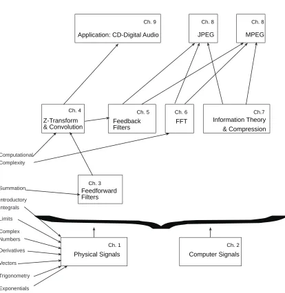
This book covers much of the mathematical foundations for understanding signals and signal processing; however, it is assumed that you are familiar with topics such as complex numbers, trigonometry, derivatives, vectors, the basic idea of integrals, infinite series, and basic physics (mass, acceleration, force, etc). Figure 0.1 shows these prerequisites in the context of this book’s chapters.

(17)

PREFACE

Application: CD-Digital Audio

Ch. 9

JPEG

Ch. 8

MPEG

Ch. 8

Ch. 5

FFT

Ch. 6

Information Theory & Compression

Ch.7

Z-Transform & Convolution

Ch. 4

Feedforward Filters

Ch. 3

Physical Signals

Ch. 1

Computer Signals

Ch. 2

Derivatives

Trigonometry Limits Complex Numbers Summation Introductory Integrals

Vectors Computational Complexity

Exponentials

[image:17.612.97.511.233.659.2]

Feedback Filters

(18)

PREFACE

applications that produce tangible changes on digital signals — it connects mathematics to

bits.

In the past, this book has been used in a wide range of signal computing courses, from those that place little emphasis on programming, to some that required Matlab implemen-tation, and in others that used C++ or the Java Media Framework.

So, this book and the concepts within can be learned without any explicit knowledge of low level programming in languages like C, C++, or Java. Most of the exercises use an online, free tool known as Java Digital Signal Processing (J-DSP) in order to put together block diagrams using signal processing techniques. Most of the problems involving J-DSP require no background in any type of programming.

However, we also provide problems for students that have varying levels of programming expertise (for example, you may have already taken an algorithms or data structures class). If you have some programming expertise, we provide problems that use simple Java methods (or functions) in the J-DSP environment. J-DSP provides a coding template for you to use, in which you can fill in your own simple manipulations of variables in the J-DSP environment using Java and use block diagrams to manipulate signals further. In this way, you can focus on the implementation of different algorithms, not the overhead involved in getting multimedia code working. If you have more experience in programming, we provide problems asking you to write small programs in your choice of a “lower level” language (such as C, C++, or Java).

About This Book

This book is divided into nine chapters. Chapters include self-test questions and review ex-ercises scattered throughout, so we suggest that you go through all the material sequentially (or, at least, do the self-test exercises in each section). Answers are provided at the back of the book. Each chapter concludes with written or programming assignments and pointers to additional readings.

If you read the PDF version of this book, you will find that it is extensively hyper-linked. This includes links from exercises to their answers, links to resources on the web, and links from the table of contents, list of figures, index, etc. to their respective locations.

(19)

PREFACE

Typographical Conventions

There are no real “standards” for much of the notation that is used in digital signal pro-cessing; depending on which textbook you read, you will encounter different typographical conventions. In this textbook, we have chosen the following:

j √₋1

t continuous time; units typically seconds

x(t) a real-valued function of continuous time (physical signal) f continuous frequency; units cycles/second or Hertz (Hz)

T an interval of time; often T = 1/f, meaning the period of a signal f0 a particular frequency; subscript may vary depending on use

ω continuous angular frequency; units radians/second

ω0 a particular angular frequency; subscript may vary depending on use

ω0 apparent (continuous angular) frequency, as a result of aliasing

n discrete time or sample number; dimensionless, but you can think of the units as being “samples”

x[n] a function of discrete time; may be real-valued (sampled signal) or discrete valued (quantized/digital signal)

ˆ

f discrete frequency; units cycles/sample ˆ

f0 a particular discrete frequency; subscript may vary depending on use

ˆ

ω discrete angular frequency; units radians/sample ˆ

ω0 a particular discrete angular frequency; subscript may vary depending

on use

Multimedia and Sensation

“What can give us surer knowledge than our senses? With what else can we better distinguish the true from the false?” Lucretius

Humans, like any other organisms, depend on their senses to provide information critical to their development and survival. Over time, life has evolved sophisticated systems for capturing information about the physical world. The first senses were almost certainly chemical — what we would call taste or smell. These senses have a number of drawbacks: they typically require close physical presence or even direct contact, they have poor temporal resolution (you can tell that someone was cooking onions, but not when), and they have poor spatial resolution (from where is that bad smell coming?). Other senses — hearing, seeing, electrical senses that fish have, magnetic senses that birds have — allow us to gather information remotely from the information source.

(22)

1. SIGNALS IN THE PHYSICAL WORLD

fashion. But what is useful? The answer to this question depends on the user, and central to the user is how his or her sensory system works.

1.2

Sensation and Perception

Regardless of the sensorymodality, all senses have one thing in common: they are composed of cells which are responsive to some property of the phys-ical world and whose responses are interpreted by a nervous system to construct a model of the world. In other words, the world does not “look” like our perception. Our perception is a construct; an inter-pretation.

For example, consider sight. Our environment is constantly bathed in a sea of radiation, which we can think of as sinusoidal waves of varying wave-length, ranging from very long (radio waves) to very short (X-rays, gamma rays), and amplitude. Some of this radiation is absorbed by objects and some is reflected, depending on the objects’ properties. The “goal” of our visual system isnot to provide us with information about reflected energy. Our visual sys-tem has evolved in tandem with the rest of our ner-vous system for the purpose of extracting useful

in-Important Terms:

color constancy our ability to perceive object color independent of light source qualities.

cone a photoreceptor that supports color vision.

luminance measure of visible light

strength.

photoreceptors sensory cells in the

retina.

retina Layer of sensory and other neurons at the back of the eye.

rod a photoreceptor that supports low-light-level vision.

trichromatic vision construction of

color sensation from measurement of three primary colors.

formation about objects’ properties based on reflected radiation. In this respect, it is much like a remote-sensing satellite and ground data analysis system: we want to know about crop conditions, we gather reflected light data at a number of wavelengths, and then we analyze the data to produce a report on crop conditions. We don’t really care about the reflected light; it is merely a means to an end.

Likewise, when we “see” a chair, what we perceive is no more a chair than the word “chair” is a chair. It is aninternal representation of a chair — a useful representation, which can allow us to recognize the object’s purpose, location, size, composition, etc., but a representation nonetheless. What we perceive about the world is at least as much a psychological issue as a data acquisition one. For brevity’s sake, however, we will confine ourselves in this section to discuss the basics of “low-level” sensory organs, rather than high-level perceptual issues. Our eyes are made up of an optical system and a sensory system. The sensory system — the retina — is composed of a number of different kind of nerve cells arranged in well-structured layers. We won’t go into the details of the eye’s structure, but instead concentrate on one class of cells: the photoreceptors.

(23)

1. SIGNALS IN THE PHYSICAL WORLD

wavelengths between roughly 400 nanometers (400_×10−9 _{meters) and 700nm — this from}

an electromagnetic spectrum that covers 1_×10−6nm to thousands of kilometers.

Our eyes have photoreceptors specialized for color vision at high (daytime) light levels (called cones) and photoreceptors specialized for low (nighttime) light levels (called rods). There are three cone types, each with a pigment sensitive to a different range of light wave-lengths. These are usually termed red, green, and blue, though the correspondences to these colors is not exact. The fact that our visual system combines measurements of three “colors” of light to form our perception of color is known as trichromatic vision.

We do not experience light as a set of intensity (luminance) measurements at a variety of light wavelengths, however. We experience light as having color. Color is a complex psychological issue, and it is still not understood exactly how this is achieved. A simple proof-by-contradiction of the idea that the color we see is the “color” of the light hitting our eyes is the observation that we see objects as having the same color under a wide range of lighting conditions (morning sunlight, afternoon sunlight, incandescent lighting). In each of these circumstances, the light reflected from the objects around us is very different because the illuminating light is different. The fact that our perception of color is more characteristic of the objects’ surface properties than the illuminating light is called color constancy. Again, our perceptual system acts to give us information about things, not measurements of incoming data.

Similar observations can be made of our sense of hearing. Sound is made of moving waves of varying air pressure, in a manner analogous to ripples on a pond. These waves are eventually transduced by auditory neurons, each sensitive to a relatively small range of frequencies (low pitched sounds, high pitched sounds — the full range of audible sounds). Yet, we do not perceive a set of signal strengths, just as we don’t for light.

Even more extraordinarily, though our sensors for sound and light are distinct and very different, we don’t have separate sensations of hearing and vision. Instead, we perceive the world as a unified whole, with sound and appearance being properties of the objects around us. Our brains fuse the incoming sensory stimuli and construct asynthetic experience.

All of the foregoing is of course a great simplification of how these systems actually work. However, these issues have great impact on the design of computer multimedia systems, because the main point of such systems is delivering a particular user experience. In the following sections, we will outline first how computer systems can generate images, then delve deeper into how we can develop a more precise, mathematical view of sound. This mathematical view will be essential to our understanding of computer representation and manipulation of multimedia information.

(24)

1. SIGNALS IN THE PHYSICAL WORLD

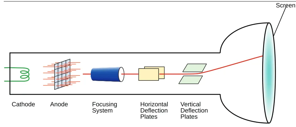
Screen

Cathode Anode Focusing System

Horizontal Deflection Plates

[image:24.612.66.539.85.288.2]

Vertical Deflection Plates

Figure 1.1: Schematic diagram of a CRT.

1.3

Computer Video Displays

The two most prevalent computer displays are cathode ray tubes (CRTs) and liquid crystal displays (LCDs); we’ll just discuss CRTs here (while they are becoming rarities, their operation is more accessible for our purposes here). A simplified CRT is sketched in figure1.1. It is composed of an electron gun, which generates cathode rays (aka, “electrons”). In this gun, a metal cathode is heated to cause electrons to “boil off;” they are accelerated toward the screen by a positively-charged anode (or possibly by charging the screen itself), which attracts the negatively-charged electrons. In between the anode and the cathode is a negatively-charged control grid. By varying the charge on the control grid, the intensity of the beam can be varied in a manner analogous to the way that a faucet valve controls the flow of water.

After leaving the electron gun, the flow of elecrons is focused into a narrow beam by an electrostatic or magnetic focusing system. The focused beam then passes by deflection plates, which can “steer” the beam magnetically to hit any part of the screen.

The screen itself is coated with one (for B&W) or more (for color) phosphors: chemicals which glow (emit visible light) when struck by electrons. Different phosphors emit different light wavelengths, and so multiple phosphors can be used to produce the perception of color images (typically by combining red, green, and blue phosphors). Another property of phosphors ispersistence: how long it will glow after an impinging electron beam is removed. Low persistence phosphors will require that the screen image be refreshed more often (by repainting the screen with the electron beam); otherwise, the display will flicker. On the other hand, a high persistence phosphor will glow longer, and so will produce blurry moving images.

(25)

1. SIGNALS IN THE PHYSICAL WORLD

Figure 1.2: Interlaced (left) and non-interlaced (right) raster scanning.

The horizontal and vertical deflection systems work in concert with the control grid to move the beam across the screen while varying its intensity. When the beam moves across the screen horizontally, its intensity is varied in proportion to the desired light intensity. While the deflection system resets to the beginning of the next horizontal line, the beam is turned off. This is called horizontal retrace.

Subsequent lines are painted on the display in a similar manner until the bottom of the screen is reached — this is oneframe. At that point, the beam is turned off and the deflection system resets itself to the beginning of the top screen line; a process called vertical retrace.

For computer displays, a frame is usually displayed in between 1/60 and 1/80 of a second (though some displays have higher refresh rates). Typically, such displays are non-interlaced (figure 1.2, right). Analog televisions, on the other hand, have interlaced displays (left). Interlaced raster scanning involves painting all of the odd scan lines in about 1/60 of a second, then a vertical retrace, and a painting of the even lines. This allows the TV 1/30 of a second to display an entire frame and yet still presents a flicker-free image (because every other line is refreshed every 1/60 of a second).

This explains how a greyscale display works. But, what about color? A color display requires three different phosphors, usually considered to be red, green, and blue (RGB). In color monitors, three electron guns are used — one dedicated to each color. The guns are aligned so that their beams strike slightly different spots on the screen. The three phosphors are laid down in a pattern so that each color gun’s beam will hit the appropriate phosphor for each pixel. By varying the intensity of each beam appropriately, control of the relative mix of the three primary colors (and thus the perceived color) and the overall brightness is possible.

1.4

Multimedia System Operation

(26)

1. SIGNALS IN THE PHYSICAL WORLD

1. They must support appropriate user perception of the media — provide output media and represent (code) media in such a way that the output seems natural.

2. They must be able to retain media — store it and provide efficient access (perhaps in a database).

3. They should allow users to reason about media information. If the goal is greater than a digital television or radio, then users must be able to manipulate the media.

4. They must be capable of transmitting media between machines. This can have signifi-cant impact on networking, resource allocation, and synchronization of activity across geographically distributed computer systems.

All of these place a high demand on computer power. For example, let’s assume that we encode audio information as 8 bits per sample at 8000 samples per second (this would be considered very low quality). How many bits per second is that (answer inA.1#1)? Perhaps that doesn’t sound too bad, so let’s consider video. Let’s say we encode each frame in a video stream as 1000x1000 pixels, 24 bits/pixel, and 30 frames/second. How many bits per second is that (answer in A.1#2)? Even if we were to achieve an extremely high compression ratio of 1/500, this would still mean more than 1 million bits/second.

On the one hand, we can attack this problem through faster hardware. But you should be well aware by this time that the difference between a good algorithm and a bad one can be the difference between an application which places very little load on a modest CPU and one which takes all the power of a supercomputer. That is what we will be focusing on here: developing the mathematical underpinning for developing efficient multimedia signal processing algorithms.

1.5

Vibrations and Sound

For much of this book, we will focus on sound when talking about signals. The reason we do this is that sound is simpler than video. Sound is a one-dimensional function of time (amplitude versus time), while video is at least a three-dimensional function of time (intensity at each x and y pixel location as a function of time for greyscale; R, G, B values at each x and y pixel location as a function of time for color).

Sound is carried by pressure waves in the air. These pressure waves can be generated by a variety of different sources. Ideally, the human ear responds to anything that vibrates between about 20 Hz and 20 kHz. A stereo speaker in a home theater system generates sound by vibrating a flexible cone. The human vocal tract generates sound by rapidly opening and closing a muscle called the glottis as air passes through it from the lungs. Musical instruments resonate at specific frequencies depending on the width and length of strings or pipes.

(27)

1. SIGNALS IN THE PHYSICAL WORLD

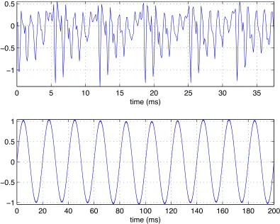
0 5 10 15 20 25 30 35

−1 −0.5 0 0.5

time (ms)

0 20 40 60 80 100 120 140 160 180 200

−1 −0.5 0 0.5 1

[image:27.612.109.504.111.427.2]

time (ms)

Figure 1.3: Real periodic signals. Top: human speech of the vowel ‘a’ as in ‘bat.’ Bottom: ringing of a tuning fork.

tract (the sound ‘a’ like in bat). In each case notice that the some portion of the wave repeats; repeating signals are commonly calledperiodic. This phenomenon has spurred scientists and mathematicians to develop standard means of representing periodic signals.

As we will see, it turns out that any periodic signal can be represented as a weighted sum of harmonically related sines and cosines (sinusoids at frequencies that are integer multiples of each other). If a periodic signal has a period ofT0 (where period is merely the reciprocal of

frequency, so T0 = 1/f0), it can be represented by a weighted sum of sinusoids at harmonics

of T0, namely sinusoids with periods of T0, 1₂T0, 1₃T0, 1₄T0, · · ·. This is potentially very

powerful! It means that if we know the period of any repeating function, we can represent it by a discrete set of weights (one weight for each harmonic).

(28)

1. SIGNALS IN THE PHYSICAL WORLD

The reason sines and cosines occur so often in nature is due to the physics of the way objects vibrate. When an object is acted on by a force, the way the object moves (its displacement) is a function of its velocity and acceleration. When solving for the exact displacement equation, x(t), we often end up with an equation of the form,

d2_x(t)

dt2 =−Cx(t) (1-1)

where C is some constant and d2_dx_t(2t) is the acceleration of the object. This kind of equation — which relates a derivative of something to itself — is called a differential equation. We bet you didn’t know they were that simple! To solve a differential equation, we look for a function, x(t), that will satisfy the equation. This is analogous to solving an algebraic equation, where we look for a number that can be substituted for a given variable. The only difference is that numbers fall along a one-dimensional number line (unless we’re talking about complex numbers), while there is no such neat number line for all possible functions. So, we need to find a function, x(t), whose second derivative is proportional to itself. Can you think of one or two (answer in A.1#3)?

Luckily, people have been working with functions and differential equations for a while, and so finding such functions is not difficult. For example, consider sinusoids. The first and second derivatives of sinωtare:

d

dtsinωt=ωcosωt (1-2)

d2

dt2 sinωt=

d

dtωcosωt =−ω

2_sin_ωt _(1-3)

Therefore, differential equation (1-1) describessimple harmonic motion: sinusoidal vibra-tion of a simple object. Sinusoids occur naturally in the real world when an object is acted on by a force! More complicated forces and objects result in more complicated differential equations, but they almost always involve sines and cosines.

Sinusoid Phase

Because sines and cosines are so powerful it is necessary to represent them as neatly and compactly as possible. Above we saw why sinωt occurs naturally. The same argument can be used for cosωt. In fact, cosine is just a delayed version of sine, as cosωt= sin(ωt+π/2). So, a more general solution to (1-1) would be:

x(t) = sin(ωt+φ) (1-4)

(29)

1. SIGNALS IN THE PHYSICAL WORLD

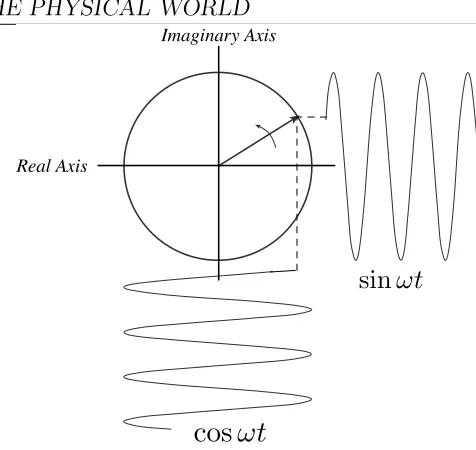
cos

ωt

sin

ωt

Real Axis

[image:29.612.181.419.75.300.2]

Imaginary Axis

Figure 1.4: Components of a phasor are sinusoids.

Let’s use tuning forks as an example. What would happen if we hit two identical tuning forks but at different times? They would vibrate at the same frequency, but would have differing phases and amplitudes (loudnesses). If the two forks were close together, we would hear the sum of their tones. What would that sum be (answer in A.1 #6)? Simplifying this sum would be involved; we would have to remember all sorts of trigonometric identities and then crank out the algebra. Luckily, we can come up with another representation of a sinusoid which simplifies this problem considerably. In fact, much of the new math we will cover in this course is primarily focused on making the paper-and-pencil work easier.

1.6

Phasors

Instead of thinking of a sinusoid as a function which oscillates up and down, let’s think of it as something that goes round and round: a rotating vector of length a (where a is the sinusoid’s amplitude). Think of this vector rotating around the origin of the x-y plane. At any point in time, the vector makes an angle θ(t) with the positive x axis. The phase, φ, is defined as φ = θ(0) (i.e., the angle that the vector makes with the x-axis at t = 0). As figure 1.4 shows, the x and y components of the vector as it moves counterclockwise are cosine and sine functions.

(30)

1. SIGNALS IN THE PHYSICAL WORLD

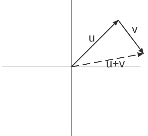
u

v

[image:30.612.187.429.92.315.2]

u+v

Figure 1.5: Graphical summation of vectors.

Complex Exponential Representation

While we used the x and y axes above as frames of reference (for considering components — sine and cosine — of the vector), we didn’t actually define what the plane was. Let’s imagine that our rotating vectors are in the complex plane, where x is the real axis and y is the imaginary axis. At any point in time, the location of a vector is therefore a complex number:

v=x+jy (1-5)

We use j here for √₋1, rather than i as you’ve probably seen before, to adhere to the convention used by electrical engineers (who use i for current). This notation allows us to represent vectors in the complex plane as complex numbers.

Note that equation1-5 is therectangular representation of complex numbers; we can also represent them in polar form (magnitude and angle), written as R6 _θ.

Review Exercises: Complex Numbers

1. What is the sum of the two complex numbersx+jy andv+jw(answer inA.1#8)?

2. What is the product of the two complex numbersx+jy andv+jw(answer inA.1#9)?

3. Convert the complex numberz=x+jy to polar form,R6 _θ _{(answer in}_A.1_#10).

4. Multiply the two polar-form complex numbersR16 θ1 andR26 θ2 (answer inA.1#11).

(31)

1. SIGNALS IN THE PHYSICAL WORLD

unit amplitude — and let’s call thisE(θ). We know from our first discussion of the rotating vector representation that cosine and sine are the x and y axis projections of the vector, so let’s rewrite our rectangular form in the complex plane as:

E(θ) = cosθ+jsinθ (1-6)

Can we rewrite the polar form in a similar way? We need a function of θ that satisfies the same requirements as the rectangular form of equation (1-6). The derivative of (1-6) is:

d

dθE(θ) = −sinθ+jcosθ (1-7) We note that (1-7) is also just jE(θ), which is the original function times a constant. What function satisfies the condition that its derivative is proportional to itself?

E(θ) =ejθ (1-8)

d

dθE(θ) =je

jθ _(1-9)

This is the complex exponential representation. It has the property that ejθ = cosθ+ jsinθ; also called Euler’s formula (“Euler” is pronounced “oiler”). It will make our work much simpler. For example, raising the complex exponential to a power is equivalent to rotating the vector:

E(θ)k = ejθk =ejθejθ_{· · ·}ejθ=ejkθ (1-10)

As you can see in (1-10), raising E(θ) to the kth _{power is equivalent to multiplying the} angle θ by k in the complex exponential.

The complex exponential ejθ has unit magnitude. The representation for a general com-plex vector R6 _θ _{is therefore} _Rejθ_{. So, we see that the sine and cosine representation is the} rectangular form, and the complex exponential is the polar form.

E(θ) = Rejθ (polar form) (1-11)

E(θ) = Rcosθ+jRsinθ (rectangular form) (1-12)

Self-Test Exercises

1. Multiply the two complex sinusoidsz1 andz2 (answer inA.1#12).

2. The complex conjugate is indicated byz∗_{. If}_z₌_x₊_jy_,_z∗₌_x

−jy. What is the complex conjugate of the complex sinusoid,z=Rejθ _{(answer in}_A.1_#13)?

3. Answer the following forz=x+jy(answers inA.1#14):

(a) What isz+z∗_?

(b) What isz₋z∗_?

(32)

1. SIGNALS IN THE PHYSICAL WORLD

Going back to (1-10), we can now write an expression for acomplex sinusoid as a function of time (a rotating complex exponential). The angle of the sinusoid is a function of time, θ(t) =ωt, where ω is its frequency (just as for our original sinusoids):

ejθ(t) =ejωt (1-13)

This rotating complex sinusoid is called a phasor (with apologies to Captain Kirk). The phasor representation is extremely powerful. Just as with sines and cosines, it turns out that

any periodic function can be written as a unique sum of phasors. Notice that phasors are complex functions but that we can add them in special ways to represent completely real functions. For example,

f(t) =ejωt+e−jωt

= cosωt+jsinωt+ cos₋ωt+jsin₋ωt Use Euler’s formula = cosωt+jsinωt+ cosωt₋jsinωt simplify₋ω

= 2 cosωt

where we have used odd and even symmetry properties of sinusoids, (sin₋x=₋sinx) and (cos₋x = cosx). The function f(t) was represented as a sum of complex exponentials but had no imaginary component! In fact, sinusoids are often represented using complex exponentials.

cosx= e

jx₊_e−jx

2 (1-14)

sinx= e

jx₋_e−jx

2j (1-15)

Practical Example: Tuning a Guitar

When a person tunes a guitar, they usually tune just the lowest string to a reference (a pitch pipe, for example). Then, they finger that string to produce the same note that the next higher string should. If the second string does produce the same tone, they can hear that. If the second string is out of tune, it will produce a slightly different tone, and they can hear

beating. Beating is what results when two sinusoids at different frequencies are added. Previously, we added two sinusoids at the same frequency, and saw that the result is another sinusoid at that same frequency. That is the case when the second string is in tune. Let’s now add two complex sinusoids with slightly different frequencies, ω and ω+δ, where the difference between the two frequencies isδ ω:

a1ejωt+a2ej(ω+δ)t=a1ejωt+a2ejωtejδt

= (a1+a2ejδt)

| {z }

low frequency

ejωt

|{z}

high frequency

(33)

1. SIGNALS IN THE PHYSICAL WORLD

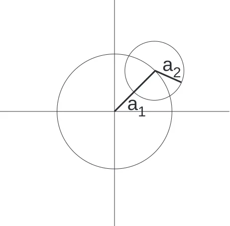
a

1

a

2

Figure 1.6: Phasor representation of beating.

0 0.5 1 1.5 2 2.5 3

−2 −1.5 −1 −0.5 0 0.5 1 1.5 2

[image:33.612.191.422.92.319.2]

time, seconds

Figure 1.7: Amplitude vs. time representation of beating.

This has the form of a complex sinusoid of frequency ω and amplitude that is a function of time, a1 +a2ejδt, that varies with a frequency of δ. Figure 1.6 presents the graphical

version of this, which looks like a top view of the amusement park “octopus” ride. There are times when the ejδt _{adds a factor of up to} _a

2 to the first sinusoid and times when it

subtracts a factor of up to a2. The result is the beating waveform seen in figure 1.7 (in this

(34)

1. SIGNALS IN THE PHYSICAL WORLD

MATLAB and Sound Files

• A MATLAB .m file for demonstrating beating is available at http://faculty. washington.edu/stiber/pubs/Signal-Computing/beating.m.

• Audio files to demonstrate beating: a 1000Hz sine wave athttp://faculty.washington. edu/stiber/pubs/Signal-Computing/1000Hz.au, a 1005Hz sine wave at http:// faculty.washington.edu/stiber/pubs/Signal-Computing/1005Hz.au, and their sum, at http://faculty.washington.edu/stiber/pubs/Signal-Computing/beating.au.

Frequency and Period

Until now, we’ve been using ω as the symbol for the speed of rotation of a phasor. If t is in seconds (which we will assume is always the case), then the phasor rotates ω/2π times in one second, or once in 2π/ω seconds. Remembering that our exponential representation corresponds cosωt+jsinωt, we see that each of these rotations corresponds to 2π radians in the oscillation of a sinusoid, and so its units must be radians/second. We will call this

angular frequency, as it is the rate of change of the phasor’s angle per second. However, when we speak of periodic physical signals, it is more convenient to speak of the number of times that the signal repeats per second: cycles/second or Hertz. We will use f to refer to frequencies expressed as Hertz. Since one cycle is 2π radians, we can convert between these two units as ω = 2πf. In this book, we will use whichever units are most convenient for each topic; you’ll need to note which is in use.

If ω and f are the number of radians or cycles of a sinusoid per second, then their reciprocals are the number of seconds per radian or cycle of rotation. Seconds per radian is only infrequently used, so we only define a symbol for seconds per cycle, T = 1/f = 2π/ω. This is the period of a signal in seconds.

1.7

Spectra

Let’s return to our discussion ofharmonics, but now using complex exponentials. We stated earlier that any periodic function could be represented by a sum of weighted harmonics. Let’s start with a sum of two sinusoids. Let’s call the first sinusoid’s frequency ω0 and the

second’s ω1 = mω0, m = 2,3, . . .. Their sum is a0ejω0t+a1ejmω0t, and there’s nothing we

can do to simplify this equation. This “failure to simplify” is not a result of our lack of mathematical sophistication — there truly is no simpler representation. Another way of saying this is that sinusoids at different frequencies are independent or orthogonal to each other. In general, if we add a large number of harmonics together, their sum is:

N

X

k=0

akejkω0t (1-17)

You’ll note that the k = 0 term of this summation has the value a0 for all time; this is

(35)

1. SIGNALS IN THE PHYSICAL WORLD

integer multiples (harmonics) of ω0, the fundamental frequency. Note that a sinusoid with

frequency kω0 has a period of 2π/(kω0) = T0/k — it repeats k times in T0 seconds. This

means it also repeats every T0 seconds, and since each term in the summation repeats every

T0 seconds, the whole summation repeats that often, and therefore the period of the signal

represented by the summation is T0. As we said before, such a summation can in fact be

used to represent any periodic function of time. The series of weights, ak, is known as the

Fourier Series. ThisFourier series is one of the most important and fundamental principles of signal processing. It allows us to look at the spectrum of a signal.

You should be familiar already with the term “spectrum” as used to describe the con-tinuous band of colors that white light (sunlight) can be broken into — a rainbow. From physics, you know that each color corresponds to a specific frequency of the visible spectrum. Hence, the decomposition of white light into colors is actually a form of frequency analy-sis. Frequency analysis involves the decomposition of a signal into its frequency (sinusoidal) components; this is also called spectral analysis. The multimedia signal waveforms we are concerned with here are basically functions of time.

At this point, you should recognize that the Fourier series represents the spectrum of a periodic signal. It (and other tools) decomposes signals into spectra defined in terms of sinusoidal (or complex exponential) components. With such a decomposition, a signal is said to be represented in the frequency domain; otherwise, usually it is in the time domain. For periodic signals, such a decomposition is the Fourier Series. For infinite signals (with finite energy), the decomposition is called a Fourier Transform. For finite, discrete signals, the decomposition is the Discrete Fourier Transform. Recombining the sinusoidal components to reconstruct the original signal is basically a Fourier synthesis problem or inverse Fourier analysis.

The weights, ak, of the Fourier Series are usually complex valued. To explain the deriva-tion of the Fourier Series, we therefore need to look at vectors in the complex plane.

1.7.1

Interlude: Vectors

Here is a list of vector operations, most of which you are likely already familiar with. Let v and w be arbitrary vectors and ~x, ~y and ~z be an orthogonal basis (the component vectors that define the coordinate system, which for 3D Cartesian coordinates would be unit vectors parallel to the X, Y, and Z axes). We can then define the following:

1. Projection of a vector onto the basis vectors (you may know these as the components

of the vector)

vx=hv, ~xi

vy =hv, ~yi (1-18)

vz =hv, ~zi

(36)

1. SIGNALS IN THE PHYSICAL WORLD and

wx =hw, ~xi

wy =hw, ~yi (1-20)

wz =hw, ~zi

(1-21)

2. Expressing a vector using the basis (i.e., as the sum of its components)

v=vx~x+vy~y+vz~z (1-22) w=wx~x+wy~y+wz~z (1-23)

3. Inner product of two vectors

hv,w_i=vxwx+vywy+vzwz (1-24) hv,v_i=v_x2+v_y2+v_z2 (1-25) You may be familiar with the inner product of a vector with itself as being its length squared, _|v_|2_{. When the vector is complex the inner product is defined as:}

hv,w∗_i=vxwx∗+vywy∗+vzwz∗ (1-26) hv,v∗_i=_|vx|2 +|vy|2+|vz|2 (1-27) where ∗ denotes complex conjugate.

We can also consider arbitrary functions to be more generalized forms of vectors. If f(t) andg(t) are periodic functions of a continuous time variablet with periodT, their inner product is defined as

hf, g_i= 1 T

Z T

0

f(t)g∗(t)dt (1-28)

which is normalized to one by T. Intuitively, you can think of this as a “projection” of one function onto another, or “how much” of of f is in the same “direction” as g.

4. Vector sum

v+w= (vx+wx)~x+ (vy +wy)~y+ (vz+wz)~z (1-29)

5. Distributive and commutative properties of inner products

hv+u,w_i=_hv,w_i+_hu,w_i (1-30)

hu,v_i=_hv,u_i (1-31)

6. v isorthogonal tow

hv,w_i= 0 (1-32)

7. Unit vector

(37)

1. SIGNALS IN THE PHYSICAL WORLD

1.7.2

Derivation of the Fourier Series

Here we present frequency analysis tools for continuous time periodic signals. A periodic signal is defined as:

f(t) = f(t+T) (1-34)

where t is a continuous time variable and T is the signal’s period.

The basic mathematical representation of periodic signals is the Fourier Series, which as we have seen is a weighted sum ofharmonically related sinusoids (sinusoids whose frequencies are all multiples of a single,fundamental one) or complex exponentials. This was first devel-oped in the nineteenth century by the French mathematician Jean Baptiste Joseph Fourier to describe heat conduction. Now it has extensive applications in a variety of problems encompassing many different fields.

The Fourier Series description of a periodic function f(t), with period T = 2π/ω0, is

defined as a weighted sum of complex exponentials:

f(t) = ∞

X

k=−∞

ckejkω0t (1-35)

We may think of the exponential signals (or phasors)

ejkω0t_, _k₌_{. . . ,}₋_2,₋_1,_0,_1,_{2, . . .} _(1-36)

as a set of basis vectors, whereω0 = 2π/T is the frequency of the phasor in radians/second.

By our earlier definition, ω0 is the fundmental frequency. In a Fourier series, the periodic

functionf(t) is expressed in terms of the basis andck is the projection of f(t) onto the basis ejkω0t_{, just like the projection} _v

x of a vector v onto the basis ~x. The weight, ck, tells us exactly “how much” of the signal,f(t), is a result of the frequencykω0. From equation1-28,

the inner product of f(t) and ejkω0t _is

ck =hf(t), ejkω0ti= 1 T

Z T

0

f(t)e−jkω0t_dt. _(1-37)

where the Fourier coefficients ck are called the frequency content or spectrum of f(t), k = 0,_±1,_±2, . . . ,_±∞. This spectrum is just like the familiar shorthand of writing a vector as a column or row of numbers, with the understanding that each is the coefficient of one of the basis vectors (i.e., when we writev= [123], what we actually mean isv= 1~x+2~y+3~z). This is the signal’s representation in thefrequency domain, where frequency is the coordinate (in other words, the signal expressed as a function of frequency). Similarly, f(t) is the signal’s

(38)

1. SIGNALS IN THE PHYSICAL WORLD

Alternative Derivation of the Fourier Series [Optional]

Another way to derive the formula for the ck is as follows. The aim of this derivation is to plug in the Fourier Series definition of f(t) into the equation for ck and see if we can get exactly ck back by manipulating the equation. We first multiply both sides of (1-35) by the phasor e−jlω0t _(l ₌_{. . . ,}−_2,−_1,_0,_1,_{2, . . .) and then integrate both sides of the resulting} equation over a single period [0, T],

ck = 1 T

Z T

0

f(t)e−jlω0t_dt ₌ 1 T

Z T

0

∞

X

k=−∞

ckejkω0te−jlω0tdt

= ∞

X

k=−∞ ck

1 T

Z T

0

ej(k−l)ω0t_dt _(1-38)

Note that

1 T

Z T

0

ej(k−l)ω0t_dt₌ 1 T

ej(k−l)ω0t j(k₋l)ω0

T 0 = e

j(k−l)ω0T −₁

j(k₋l)ω0T

(1-39)

Equation (1-39) has two different solutions, depending on whether k = l or not. Let’s make the substitutionu=k₋l. So, whenk =l,u= 0, and the numerator and denominator of (1-39) are both zero. We therefore use L’Hˆopital’s rule to find the limit:

lim u→0

ejuω0T ₋₁ juω0T

=

d du e

juω0T −₁

d

dujuω0T

_u₌₀

= jω0T e juω0T jω0T

u=0

= jω0T jω0T

= 1 (1-40)

For the case of k ₆=l, let’s rewrite the numerator of (1-39) as cos(k₋l)ω0T +jsin(k−

l)ω0T−1. Remember thatω0 = 2π/T, and soω0T = 2π. Since bothk andl are integers and

k ₆= l, their difference is an integer; let’s call that integer m. The numerator then becomes cos 2πm+jsin 2πm₋1. We know that cos 2πm= 1 and sin 2πm= 0, and so the numerator is zero. On the other hand, the denominator of (1-39) is j2πm₆= 0, and so (1-39) is zero.

In summary,

1 T

Z T

0

ej(k−l)ω0t_dt ₌

1 k =l

0 k ₆=l (1-41)

(39)

1. SIGNALS IN THE PHYSICAL WORLD

complex sinusoids at different frequencies are orthogonal (and so, by extension, can serve as an orthogonal basis).

Using (1-41), equation (1-38) becomes

1 T

Z T

0

f(t)e−jlω0t_dt ₌_c

l, l =. . . ,−2,−1,0,1,2, . . . (1-42)

We got the same result as (1-37).

Real-Valued Signals

In general, the Fourier coefficients ck are complex valued. If the periodic signal f(t) is real valued (the kind of signals we’re concerned with here), the ck satisfy the condition,

ck=c∗−k (1-43)

Consequently,

|ck|2 =|c∗−k|

2 _(1-44)

Sinceckis the (amplitude) spectrum off(t),|ck|2 is thepower spectrum. Equation (1-44) tell us that the power spectrum is a symmetric (or “even”) function of frequency. Also, when f(t) is real, we can further decompose the Fourier Series. Equation (1-35) becomes

f(t) = ∞

X

k=−∞

ckejkω0t

=c0+

∞

X

k=1

ckejkω0t+ −∞

X

k=−1

ckejkω0t (split sum into 0/+/- parts)

=c0+

∞

X

k=1

ckejkω0t+ ∞

X

k=1

c−ke−jkω0t (distribute -1 into second sum)

=c0+

∞

X

k=1

[ckejkω0t+c−ke−jkω0t] (combine common sum)

=c0+

∞

X

k=1

[ckejkω0t+ (c∗−ke

jkω0t₎∗_] _{(double conjugate)}

=c0+

∞

X

k=1

[ckejkω0t+ (ckejkω0t)∗] (real signal: ck =c∗−k)

=c0+ 2

∞

X

k=1

Re[ckejkω0t] (a+a∗ = 2 Re(a)) (1-45)

With your help in the next self-test exercise, we get

f(t) =c0+ 2

∞

X

k=1

Re(ck) coskω0t−2

∞

X

k=1

(40)

1. SIGNALS IN THE PHYSICAL WORLD where

Re(ck) = 1 T

Z T

0

f(t) cos(kω0t)dt (1-47)

Im(ck) = − 1 T

Z T

0

f(t) sin(kω0t)dt (1-48)

from (1-37) and Euler’s formula. You can view equations 1-47 and 1-48 as the projection of f(t) onto cosine and sine functions in the same way that the previous definition ofck was the projection off(t) onto complex exponentials. This representation ofck does not require any complex number arithmetic, but it is often more cumbersome to carry out the integration using cosines and sines, rather than phasors.

Examples of periodic signals that are frequently encountered in practice are square waves, rectangular waves (both being used as timing signals in electronics), triangle waves, and of course sinusoids and complex exponentials. In the next example, we will use the Fourier series to analyze some of these.

Self-Test Exercises

SeeA.1#15–16for answers.

1. Prove the relationship in (1-43).

2. From equation (1-45), derive (1-46). Hint: Use the fact that equation (1-45) is a real signal to simplify the complex multiplication.

Example: Fourier series of a general square wave

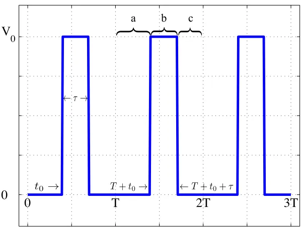
The simplest type of square wave has a 50% duty cycle: that is, 50% of the timef(t) takes on the value of 1 and 50% of the time it has the value -1. Let’s do a bit more general of a case. We will consider a train of rectangular pulses (a kind of square wave, but shifted upward and scaled so that it has a minimum of zero and a maximum of V0) with pulse duration τ

and period T seconds. This waveform can be expressed as

f(t) =

 



0 region a (nT _≤t < nT +t0)

V0 region b (nT +t0 ≤t < nT +t0+τ)

0 region c (nT +t0+τ ≤t <(n+ 1)T)

n= 0,1,2, . . . (1-49)

The waveform is plotted in figure 1.8 with example regions shown.

(41)

1. SIGNALS IN THE PHYSICAL WORLD

0

V

0

T

2T

3T

{

a b c

T+t0→ ←T+t0+τ

←τ_→

[image:41.612.154.455.102.332.2]

t0 →

Figure 1.8: A train of periodic rectangular pulses with period T, pulse width τ, and initial pulse start att0.

According to (1-37), the Fourier coefficients ck are

ck = 1 T

Z t0

0

0e−jkω0t_dt₊ 1 T

Z t0+τ

t0

V0e−jkω0tdt+

1 T

Z T

t0+τ

0e−jkω0t_dt _(1-50)

= 1 T

Z t0+τ

t0

V0e−jkω0tdt (1-51)

= V0 T

e−jkω0t −jkω0

t0+τ

t0

(1-52)

= V0 −jkω0T

[e−jkω0(t0+τ)₋_e−jkω0(t0)_] _(1-53)

In equation (1-50), the integral defining the Fourier coefficients in (1-37) has been broken into three parts for the three “segments” of the square wave: f(t) = 0 (region a, when nT _≤ t < nT +t0), f(t) = V0 (region b, when nT +t0 ≤ t < nT +t0 +τ), and f(t) = 0

(region c, when nT +t0+τ ≤ t < (n+ 1)T). The first and third terms are equal to zero,

(42)

1. SIGNALS IN THE PHYSICAL WORLD

-10π -5π 0 5π 10π

α

-0.4 -0.2 0 0.2 0.4 0.6 0.8 1

sinc(

α

)

Figure 1.9: The sinc function.

The middle steps are left for your homework; let’s skip to the result:

ck= V0τ

T

sin(kω0τ /2)

kω0τ /2

| {z }

magnitude

e−jkω0(t0+τ /2)

| {z }

phase

(1-54)

This is just the polar representation of a complex valuedck=Rejθ. The phaseθ or angle of ck is

θ=₋kω0

t0+

τ 2

(1-55)

Let’s define α = kω0τ /2, and take a look at the magnitude in (1-54). This function

oc-curs frequently enough in modern communication theory to be given a name: the sampling function, or sinc. We define

sincα= sinα

α (1-56)

We note that sincα is zero whenever α is an integral multiple of π; that is,

sincnπ = 0, n = 1,2,3, . . . (1-57)

When α is zero, the function is indeterminate, but it is easy to show that its value is unity:

sinc 0 = 1 (1-58)

(43)

1. SIGNALS IN THE PHYSICAL WORLD

continues to increase, the successive maxima become smaller because the numerator of sincα can not exceed unity while the denominator increases. Also, sincα shows even symmetry. Figure1.9 shows the sinc function.

From (1-58), we know that c0 is

c0 =

V0τ

T (1-59)

Substituting c0 and ck, k= 1,2,3, . . . into (1-45), the Fourier series of f(t) is

f(t) = V0τ

T + 2 Re

( _∞

X

k=1

V0τ

T

sin(kω0τ /2)

kω0τ /2

e−jkω0(t0+τ /2)_ejkω0t

)

(1-60)

= V0τ

T + 2 Re

( _∞

X

k=1

V0τ

T

sin(kω0τ /2)

kω0τ /2

ejkω0(t−t0−τ /2)

)

(collect exponents) (1-61)

= V0τ T

|{z}

c0

+2V0τ T

∞

X

k=1

sinc(kω0τ /2)

| {z }

ck

cos[kω0(t−t0−τ /2)]

| {z }

harmonically related sinusoids

(apply Euler’s) (1-62)

In (1-60), we have used the knowledge of this being a real-valued signal. We collected the exponents to get (1-61), then factored out the V0τ /T, applied Euler’s formula to the

exponential, and finally retained only the real part of each term of the summation to yield ( 1-62).

Now, a train of pulses is represented by an infinite number of sinusoidal waves. How well can it be approximated by a finite number? Look at figure 1.10. The solid curve shows the sum of the first 12 terms of the signal’s Fourier series; it looks like a pulse train modulated by a sinusoid. The ideal pulses are shown as dashed lines. The approximation gets better when more terms are used, as in figure 1.11.

Let’s construct the signal’s spectrum: a plot of its Fourier coefficients. We first consider |ck| expressed in terms of the fundamental frequency f0, remembering that ω0 = 2πf0:

|ck|= V0τ

T |sinc(kπf0τ)| (1-63)

The magnitude of any ck is obtained from (1-63) by using the known values of pulse width τ and signal period T = 1/f0, and selecting the desired value of k (k = 0,1,2, . . .).

Instead of evaluating (1-63) at these discrete frequencies, let us sketch the envelope of _|ck| by considering the frequency kf0 to be a continuous variable. That is, though f =kf0 can

really only take on the discrete values (the harmonic frequencies - 0, f0,2f0,3f0, . . .) we may

think ofk for the moment as a continuous variable. Whenf is zero,_|ck|isV0τ /T, and when

f has increased to 1/τ, _|ck| is zero. In fact from (1-57) when f πτ = mπ (m = 1,2,3, . . .), sinc(f πτ) = 0, which yields zeros at frequencies f =m/τ.

(44)

1. SIGNALS IN THE PHYSICAL WORLD

0

V

0

T

2T

3T

t0 t0+τ

Figure 1.10: The Fourier series for a periodic sequence of rectangular pulses. The first 12 harmonic terms in summation (1-62) are included. The ideal pulse train is shown as dashed lines. The period is T = 1, the initial point t0 = 0.5 and the pulse widthτ = 0.3333.

of rectangular pulses), versus frequency f =kf0. The magnitude of its peaks decays at the

rate of 1/k.

There are several observations which we may make that relate changes in the line spec-trum to changes in the graph of rectangular pulses given in figure 1.12. Firstly, note that the width of the envelope depends upon changes inτ, the pulse width. In fact, the shape of the envelope does not vary with changes in T; instead, changes in T correspond to changes in the frequency interval between spectral lines. If the pulse period T is increased (f0 is

decreased), the number of spectral lines between zero frequency and 1/τ increases and the amplitude of each line decreases. Figures 1.13 and 1.14 illustrate this.

A shift in the phase t0 does not change the line spectrum, that is,|ck| is not a function of t0. Thephase of the frequency components do change with the choice oft0 (we just haven’t

plotted those).

(45)

1. SIGNALS IN THE PHYSICAL WORLD

0

V

0

T

2T

3T

t0 t0+τ

Figure 1.11: The Fourier series for a periodic sequence of rectangular pulses. The sum of the first 100 terms is shown, as in figure 1.10.

Self-Test Exercise

SeeA.1#17for the answer.

1. Prove (1-58).

1.8

Problems

1. The differential equation for a tuning fork can be written as d2_dx_t2(t) = − k

Mx(t) where M is the mass of the tuning fork, k is a constant, and x(t) is the displacement of the tuning fork endpoints. Discuss how the mass of the tuning fork affects the frequency at which it vibrates. Hint: relate the given equation to equation1-1.

2. What musical instruments might be governed by properties analogous to that of a tuning fork?

(46)

1. SIGNALS IN THE PHYSICAL WORLD

k=0

k=1

k=2

k=3 k=4

k=5

k=6

k=7 k=8

0

3f

₀

6f

₀

9f

₀

V

0

τ

T

V

0

τ

2T

0

←

V

T

0

τ

|

sinc(

kπf

0

τ

)

|

c

k

|

k

Figure 1.12: The spectrum of a periodic sequence of rectangular pulses: the magnitude of ck vs. frequency f = kf0, where f0 = 1/T (light gray vertical lines). The envelope

for continuous k is plotted as the black curve. Zero points in the spectrum _|ck| are at kf0 =n/T =m/τ, m = 1,2,3, . . ..

4. A complex number can be written in rectangular coordinates as z =x+jy. Write the relations to calculate the polar form, z = (r, θ) or z =rejθ_.

5. Using Euler’s formula, express cosxand sinxas a combination of complex exponentials. Recall that Euler’s Formula is given by: e±jωt _{= cos(ωt)}_±_j_sin(ωt).

6. Find expressions for the following as complex exponentials:

(a) 1

(b) j

(c) 1 +j, (1 +j√3)/2

7. Compute [(1 +j√3)/2]2 _{and (1 +}_j)4 _{directly using:}

(a) Rectangular representations.

(b) Complex exponentials.

(47)

1. SIGNALS IN THE PHYSICAL WORLD

0 0.5 1

0 T 2T 0

1 2

! = 0.50T

0 3f0 6f0 9f0

0 0.5 1

0 T 2T 0

1 2

! = 0.30T

0 3f0 6f0 9f0

0 0.5 1

0 T 2T 0

1 2

! = 0.20T

0 3f0 6f0 9f0

Figure 1.13: The spectrum of a periodic sequence of rectangular pulses, when T is fixed and the pulse width tauvaries.

9. Express _|z_|2 _{as a function of} _z _and _z∗_.

10. Given the following equations:

x1(t) = 5 sin(2π(200)t+ 0.5π)

x2(t) = 5 sin(2π(200)t−0.25π)

x3(t) = 5 sin(2π(200)t+ 0.4π)

x4(t) = 5 sin(2π(200)t−0.9π)

(a) Using pencil and paper: Express x1(t) through x4(t) as complex exponentials.

(b) Create the sum sinusoid, x5(t) = x1(t) +x2(t) +x3(t) +x4(t). Express x5(t) as a

sum of complex exponentials.

(c) Using complex exponentials, express the amplitude and phase of x5(t) (use pencil

and paper with the aide of a graphing calculator, spreadsheet, or MATLAB).

11. What is the period of e−jπ4t+e−j

π

2t ?

(48)

1. SIGNALS IN THE PHYSICAL WORLD

0 0.5 1

0 T 2T 0

1 2

T = 2!

0 3f0 6f0 9f0

0 0.5 1

0 T 2T 0

1 2

T = 3!

0 3f0 6f0 9f0

0 0.5 1

0 T 2T0

1 2

T = 4!

0 3f0 6f0 9f0

Figure 1.14: The spectrum of a periodic sequence of rectangular pulses with fixed pulse width tauand varying period T.

13. Implement a Complex class for representing complex numbers in an object oriented programming language (C++, C#, Java, python, etc.). Your class should include at least the following methods:

• add()

• multiply()

• real()

• imag()

• magnitude()

• angle()

Document your code so that this class could be used by someone else. Write a test program that exercises all of this class’ methods.

14. Derive equation (1-54) from equation (1-53).

(49)

1. SIGNALS IN THE PHYSICAL WORLD (a) The sinusoid

x(t) = cosπ 3t

(b) The sawtooth waveform

x(t) = t_{− b}t_c

(c) The rectified wave

x(t) = _|cos(π 3t)|

1.9

Signal Computing: Digital Signals in the Software Domain